Data-Driven Low-Dimensional Modeling and Uncertainty Quantification for Airfoil Icing

Abstract

The formation and accretion of ice on the leading edge of an airfoil can be detrimental to aerodynamic performance. Furthermore, the geometric shape of leading edge ice profiles can vary significantly depending on a wide range of physical parameters, which can translate into a wide variability in aerodynamic performance. The purpose of this work is to explore the variability in airfoil aerodynamic performance that results from variability in leading edge ice shape profile. First, we demonstrate how to identify a low-dimensional set of parameters that governs ice shape from a database of ice shapes using Proper Orthogonal Decomposition (POD). Then, we investigate the effects of uncertainty in the POD coefficients. This is done by building a global response surface surrogate using Polynomial Chaos Expansions (PCE). To construct this surrogate efficiently, we use adaptive sparse grid sampling of the POD parameter space. We then analyze the data from a statistical standpoint.

1 Introduction

Leading edge wing ice can present a significant safety hazard to pilots. Wing ice shapes are often sharp and jagged in profile and rough in surface texture; both of these characteristics tend to induce flow separation at angles of attack which are often quite mild. This can cause stall at lower angles of attack than those to which pilots are accustomed. It is for this reason that wing icing has been identified as the cause of 388 crashes between 1990 and 2000 [1].

Equally troubling is the fact that wing icing is a process which is associated with a high degree of uncertainty in practice. If one were to analyze a database of ice shapes—regardless of whether the data come from wind tunnels, flight tests, or computation—one would usually find that the ice profile can vary significantly, depending on a wide range of physical parameters (e.g., the liquid water content of the freestream, airfoil geometry, the distribution of droplet properties, etc.). It is therefore natural to ask how airfoil aerodynamic performance is affected by variations in the ice shape. This is the main question we hope to contribute towards addressing in this work.

The approach we adopt is data driven, in the sense that all of the ice shape variations that we will explore are, in a fundamental way, derived from pre-existing databases of ice shapes. This is in contrast to prior related studies, in which the ice shape variations that were examined were generated in a somewhat heuristic fashion [2].

The framework we adopt includes a combination of techniques from low-dimensional modeling and uncertainty quantification. Specifically, given a database of ice shapes, we first identify a low-dimensional set of shape parameters by using the Proper Orthogonal Decomposition (POD) of the dataset. This gives us both a method for generating and studying artificial ice shapes as well as a way to assess the statistical variation of our dataset.

Based on the variation in the data, we select a parameterized range in POD space to perform uncertainty quantification (UQ). We generate artificial ice shapes by taking linear combinations of the POD modes, and study the effects on aerodynamics by meshing the resultant airfoil and computing its aerodynamic properties using an in-house flow solver. In order to perform the UQ efficiently, we fit a surrogate function to the data using a polynomial basis that is orthogonal to the input parameter probability distribution; this method is known as Polynomial Chaos (PC). We use an adaptive sparse grid algorithm as our collocation method.

2 Uncertainty Quantification for Airfoil Icing: Methodology

In this section, we describe the various techniques we apply. Specifically, we first show how we identify low-dimensional models for icing datasets. These models will form the input parameter space for our UQ studies. Next, we discuss the flow solver we will be using for the iced airfoil calculations. The aerodynamic quantities we derive from these flow calculations form the response function outputs in our UQ studies. Finally, we describe the methods we will be using to quantify uncertainty in our response function, as a result of uncertainty in our input parameter space.

2.1 Low-Dimensional Modeling using POD

The space of all possible ice shapes contains an infinite number of degrees of freedom. However, for exploring parameter space, we wish to restrict our study to a relatively small number of parameters that describe likely ice shapes. The approach taken here is to consider a subspace of possible ice shapes, determined from data, either from simulations (§3) or experiments (§4). In particular, for a given dataset of ice shapes, we determine a low-dimensional subspace that optimally spans the data using Proper Orthogonal Decomposition (POD) [3].

Denote the vector of parameters governing a particular ice shape by $x\in\mathbb{R}^{N}$ (we will have more to say about what $N$ is and how we get it soon). We wish to approximate any $x$ as a linear combination of some basis vectors $\psi_{i}$, called POD modes:

$$x\approx\sum_{i=1}^{P}a_{i}\psi_{i}$$ (1)

POD gives us one way of generating the basis $\{\psi_{i}\}$ from the data. A key property is that the basis identified by POD will be able to represent the dataset better than any other linear basis, in the sense of projection error (using the standard Euclidean norm). The POD modes are determined as follows. Let $x_{j}$, $j=1\ldots M$ denote the elements in our dataset, and let ${\bf{X}}\in\mathbb{R}^{N\times M}$ be the matrix with $x_{j}$ as its columns:

$$\mathbf{X}=\begin{bmatrix}\vline&&\vline\\ x_{1}&\cdots&x_{M}\\ \vline&&\vline\\ \end{bmatrix}$$ (2)

The POD modes $\psi_{i}$ are then given by the left singular vectors of the singular value decomposition ${\bf{X}}={\bf{U}}{\bf{\Sigma}}{\bf{V}}^{T}$ (i.e., the columns of ${\bf{U}}$).

2.2 Flow Solver Description

In order to evaluate the aerodynamic characteristics for the different ice shapes considered, we need a reliable, tested flow solver. In this paper, we use use FLO103, a well-validated, in-house code for the solution of the two-dimensional Reynolds Averaged Navier-Stokes (RANS) equations developed over the course of many years by Martinelli and Jameson [4, 5, 6]. This code has also been used to perform similar aerodynamic calculations for iced airfoils in a previous study [2].

A one-equation Spalart-Allmaras turbulence model [7] provides closure for the RANS, which is capable of accurately modeling mildly separated flow near the stall regime. The discretization of the spatial operators is carried out by using a second order cell-centered finite-volume method in which the viscous stresses are computed using a discrete form of Gauss’ theorem. The key to the flow solver efficiency is a full approximation multigrid time-stepping scheme, which accelerates the rate of convergence to a steady state.

2.3 Uncertainty Quantification using PCE

The POD modeling of the ice dataset has—viewed from a UQ perspective—generated for us a relatively low-dimensional parameter space to explore. Casting this as a UQ problem has several potential benefits and uses:

• A linearly parameterized description of the ice gives us an easy and systematic method of generating new ice shapes that effectively interpolate the shapes present in our database. This makes it possible to produce and study a wide range of shapes.

• UQ tools allow us to compute and analyze the statistical relationships between our responses (aerodynamics) and our inputs (ice shapes). For example, we can look at the effect of different input distributions (eg. uniform, Gaussian, etc.), correlations between POD modes and lift coefficients, output statistics, etc.

• The UQ tools we will be using produce for us a surrogate model of the input-output behavior – we obtain a polynomial mapping between the POD modes and the aerodynamics. This can be advantageous as a predictive tool: if one wishes to know the aerodynamics of a particular ice shape that has not been studied yet, one could compute it by simply evaluating the surrogate model (assuming this ice shape is in the span of the POD basis).

Furthermore, using POD to generate our parameterization of the ice is advantageous for a few reasons:

• The POD basis outperforms any other possible linear basis of the same dimension for representing our data in the sense of projection error. In this way, it is an optimal parameterization.

• The POD coordinates are linearly uncorrelated (since the modes are orthonormal). This justifies an assumption of mutual independence amongst the parameters in our UQ study, which underlies the UQ methods we will be using.

• The POD is a general method for data-processing, which makes it amenable to analyzing other ice shape databases that we have not yet considered. Thus, our approach could be applied to other datasets as well.

Here, we detail exactly how our ice shape modeling can be formulated as a parameterized UQ study. We then present results for such a study, and analyze the statistical information that we can glean from it.

As previously noted, the UQ methods that we will be using need to be efficient, since we have a moderately high dimensional parameter space to explore. Additionally, we would like to obtain a surrogate model that explicitly describes the dependence of the airfoil aerodynamics on ice shape, which can be inexpensively sampled and analyzed for statistical correlations. As a result of these requirements, we choose to use Polynomial Chaos Expansions (PCE) as our framework for performing UQ.

We give a brief overview of this approach below; further details can be found in introductory references on PCE methods[8, 9, 10].

Let $Z=(Z_{1},\ldots,Z_{d})$ be a vector of random variables that parameterize the uncertain quantities in the ice shape. We are interested in the corresponding uncertainty of an aerodynamic quantity, represented by $y(Z)$. In our setting, $Z$ are the POD coefficients, and $y(Z)$ will be the airfoil lift and drag coefficients at a particular angle of attack, computed by FLO103.

The goal of the method is to represent $y(Z)$ in terms of some basis functions $\Phi_{i}$. Assuming (for ease of exposition) that $y(Z)$ is scalar-valued, we write:

$$y(Z)=\sum_{|i|=0}^{N}y_{i}\Phi_{i}(Z).$$ (3)

Here, $i=(i_{1},\ldots,i_{d})$ is a multi-index, and $|i|=\sum_{j=1}^{d}i_{j}$. We define an inner product on the space of functions of the random variables by

$$\left\langle f,g\right\rangle=\int_{\Gamma}f(Z)g(Z)\rho(Z)\,dZ,$$ (4)

where $\rho(Z)$ denotes the probability density function of $Z$, and has support $\Gamma$. A fundamental insight in PCE methods is to employ basis functions that are orthonormal with respect to this inner product, so that

$$\left\langle\Phi_{i},\Phi_{j}\right\rangle=\delta_{ij},$$ (5)

where $\delta_{ij}=1$ if $i=j$, and $0$ if $i\neq j$. In particular, a multivariate basis polynomial $\Phi_{i}$ may be written as

$$\Phi_{i}(Z)=\prod_{k=1}^{d}\phi_{i_{k}}(Z_{k}),$$ (6)

where $\phi_{n}$ is a (univariate) polynomial of degree $n$. The $\{\phi_{n}\}$ will be a basis of orthogonal polynomials chosen so that the orthogonality condition (5) is satisfied. In this paper, we work exclusively with uniformly distributed random variables, and so our basis polynomials are the multivariate Legendre polynomials.

The coefficients $y_{i}$ in the expansion (3) may be determined by taking an inner product with $\Phi_{j}$: because the $\Phi_{j}$ are orthonormal, we have

$$y_{j}=\left\langle y,\Phi_{j}\right\rangle.$$ (7)

Note that one could also take $y(Z)$ to be a vector of several different aerodynamic quantities of interest: in this case, the coefficients $y_{i}$ in the expansion (3) are vectors, and each component of $y_{i}$ is determined by an equation such as (7), for the corresponding component of $y$.

The important issue now is how we choose to approximate the projection integrals in (7). A possible choice is to use Gauss quadrature, in which the function $y(Z)$ is evaluated on a grid consisting of the tensor product of $n$ separate 1-D quadrature point sets in parameter space. However, this method suffers from the curse of dimensionality, since the number of required samples grows exponentially with the dimension $n$.

A commonly used alternative is to use sparse grid methods[11], in which the number of grid points used is lessened by using only a subset of the full tensor product. Another advantage is that anisotropic adaptive $p$-refinement of the mesh is possible, since nested 1-D nodes are used. In an adaptive setting, global sensitivities are calculated using total Sobol indices, which are defined for each parameter as:

$$T_{i}=\frac{\mathbb{E}[Var(y|Z_{-i})]}{Var(y)},\qquad i=1,\ldots,d,$$ (8)

Here, $Var(y|Z_{-i})$ denotes the variance of $y(Z)$ given all parameters except $Z_{i}$. This is a measure of “how much” parameter $Z_{i}$ contributes to the total variance of $y(Z)$ on average. Parameters that have higher Sobol indices contribute more to the variance of the response and hence require more refinement than parameters with lower Sobol indices.

Further details on the sparse grid approach can be found in standard references[10, 12]. In our study, we compute the sparse grids using DAKOTA, an open-source code for optimization and UQ developed by Sandia National Laboratory [13].

3 Results: Ice Shapes from Simulations

In this section, we give our first example of how the techniques just discussed may be applied to an ice shape dataset from the literature. For this example, our data consists of cross-sections from an icing simulation performed on a 3D swept wing. This data and the research related to it is described in detail in Broeren et. al. [14] and is shown in Figure 1.

Figure 1: Horn ice accretion case on the NASA CRM, from Broeren et. al.[14].

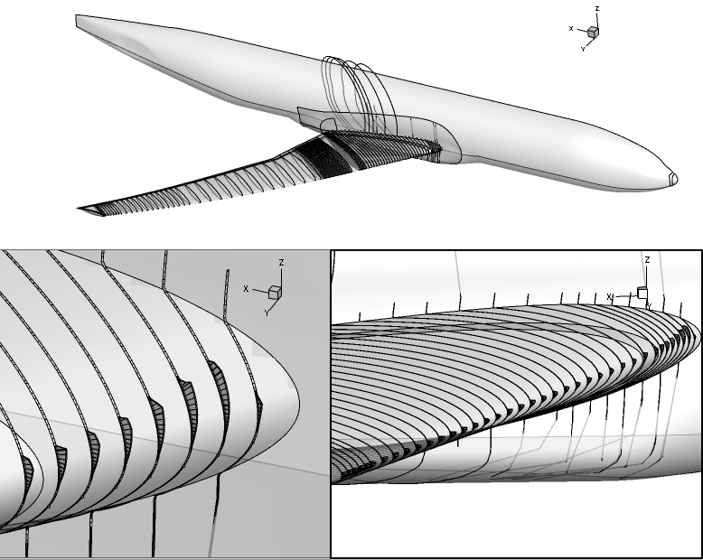
The model geometry used in this data set was the NASA Common Research Model (CRM) at 65% scale. The ice accretion model used was LEWICE3D, which is a NASA’s 3D icing code. This study represents 45 minutes of accretion time at an altitude of 10,000 ft and free stream velocity of 232 knots. The static temperature was $-4^{\text{o}}$ C, the mean volumetric diameter (MVD) was 20 $\mu$m, and the liquid water content (LWC) was 0.55 g/m³.

3.1 Modeling using POD

Our first objective is to apply the POD machinery to the data set consisting of 95 individual horn ice cross sections on the CRM wing, with the objective of identifying the most important ice shape features. We will first do a preprocessing step on our data – we will map all of the airfoil cross sections into $s$-coordinates (arc length coordinates, relative to the airfoil leading edge), so that the ice shapes may be represented as a function of a single variable.

Let us denote the horn ice height (in $s$-coordinates, normal to the airfoil) as $N_{k}(s)$, where $k$ indexes the cross-sections. A POD representation of this dataset will take the following expansion form:

$$N_{k}(s)=\overline{N}(s)+\sum_{i=1}^{M}c_{i_{k}}\psi_{i}(s),\qquad k=1,\ldots,S.$$ (9)

Here, $\overline{N}(s)$ is the height (in s-coordinates) of the mean ice shape, $c_{i}$ is the $i^{th}$ POD coefficient, and $\psi_{i}(s)$ is the $i^{th}$ POD mode.

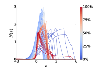
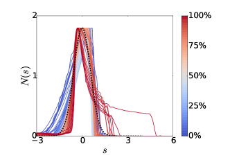
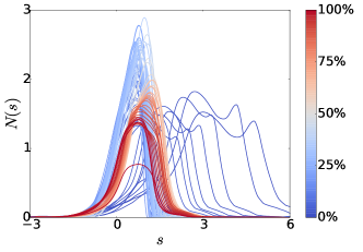
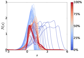
Fig. 2(a) shows the dataset. By inspection, we see that much of the variability in shape is due to differences in width, position, and height. We can account for this by scaling/shifting each of the individual ice shapes to fit a template shape, which produces Fig. 2(b). The point of doing this is to separate variations in scaling from differences in shape. As we will see, this will be reflected in our parameterization of the ice, in which three of the parameters specify scaling, and the two POD modes specify shape perturbations.

If we pre-process the data with these scalings/shiftings, the POD expansion will be:

$$N_{k}(s)=h_{k}\left(\overline{N}(a_{k}s+b_{k})+\sum_{i=1}^{M}c_{i_{k}}\psi_{i}(a_{k}s+b_{k})\right),\qquad k=1,\ldots,S.$$ (10)

In this framework, uncertainty could be accounted for by perturbing the POD coefficients:

$$a_{k} \mapsto a_{k}+\xi_{a}$$ (11)

$$b_{k} \mapsto b_{k}+\xi_{b}$$

$$h_{k} \mapsto\xi_{h}h_{k}$$

$$c_{i_{k}} \mapsto c_{i_{k}}+\xi_{c_{i}}\;\;\;\text{for $k$ = 1 ... $M$}$$

Here, the first three parameters are perturbations on the nominal positions, widths, and heights of all of the individual ice shapes. The last $M$ parameters are global perturbations on each of the POD eigenmodes. The first three parameters were chosen by scaling/shifting each individual shape so that the transformed shape most closely matches a symmetric Gaussian template $G(s)$ (which is close to the mean of the unshifted/unscaled data):

$$(a_{k},b_{k})=\arg\min_{a,b}\|N_{k}(as+b)-G(s)\|_{2}^{2},\qquad k=1,\ldots,S.$$

(a) Horn profiles unaligned.

(b) Horn profiles scaled/shifted to fit a symmetric Gaussian template centered at zero.

Figure 2: Horn profiles, unaligned and aligned. The color map denotes spanwise position along the CRM wing from root (0%) to tip (100%).

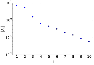
The absolute values of the POD eigenvalues are shown in Figure 3. As can be seen, there is a sharp drop-off in the magnitude of the scaled/shifted POD eigenvalues at mode 2. This implies that the first two modes capture much of the important features.

(a) Magnitude of POD eigenvalues.

(b) The mean and first 2 POD modes.

Figure 3: POD eigenvalues and modes for the scaled/shifted data.

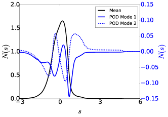
Shown in Figure 4 are original ice shapes along with their reconstructions using 1 and 2 POD modes. It can be observed that no skewness is able to be represented until 2 POD modes are used.

(a) Reconstruction (1 POD mode).

(b) Reconstruction (2 POD modes).

Figure 4: POD reconstructions of the ice. The color map denotes spanwise position along the CRM wing from root (0%) to tip (100%).

Figure 5: Spanwise variation of the POD modes.

(a) Variation of the $1^{st}$ POD mode $\in(-2,2)$.

(b) Variation of the $2^{nd}$ POD mode $\in(-2,2)$.

Figure 6: Variation of the POD modes on the mean (dashed black).

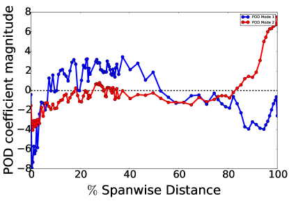
The next step in identifying the relevant parameters for a UQ study is to study the spanwise variation of the POD coefficients. Figures 5 and 6 demonstrate these properties. As can be seen, both modes are most pronounced at the boundaries, since this is where ice shapes deviate the most from the mean. The first mode has the effect of making the ice profile wider and skewed left; hence, it is largest in magnitude on the inboard portions of the wing. The second mode has the effect of skewing the ice profile right; hence, it is largest in magnitude on the outboard portions of the wing.

3.2 Airfoil Icing UQ: Five-Parameter Scenario

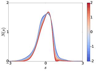
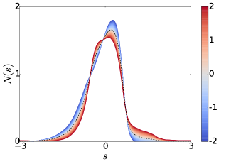
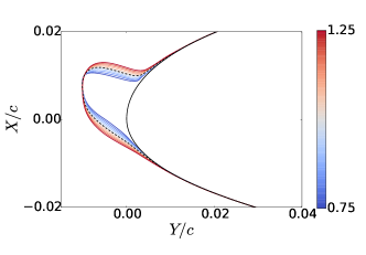
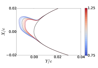
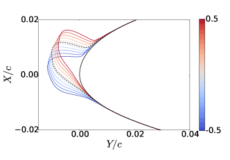
Now that we have generated a POD representation of our horn shape data, we can investigate the effects of uncertainty in the POD coefficients. As shown in Eq. (10), we have 3 scaling parameters (height, width, and position), and 2 POD coefficients, so our parameter space is 5 dimensional. We assume that all 5 of our parameters are uniformly distributed between some bounds. The ranges that we choose, as well as their independent effects on the horn shape, are displayed in Fig. 7.

(a) Variation of the width.

(b) Variation of the height.

(c) Variation of the position.

(d) Variation of the POD modes. $Inset$: POD coordinates of the ice shapes (colored) and original data (black).

Figure 7: Depiction of the ranges of each of the parameters in the 5-dimensional parameter space and their effects on the horn shape (colorbars indicate parameter ranges). Dashed black ice shape in each subplot represents the mean shape used.

3.3 Results and Discussion

Here we describe the results of the UQ investigation described in the last section. We will quantify uncertainty in the two response metrics $C_{L}$ and $C_{D}$. The airfoil cross-section used here was chosen to be the cross-section at 50$\%$ semispan of the CRM, and the aerodynamic coefficients were determined at a Reynolds number of $5\times 10^{6}$, Mach number of $0.4$, and angle of attack $\alpha=3^{\circ}$.

(a) PDF for $C_{L}$.

(b) PDF for $C_{D}$.

Figure 8: Probability density functions for two response metrics in the 5 parameter UQ study. These results required 1,103 samples in the adaptive sparse grid algorithm.

Table 1: Data correlations

	$C_{L}$	$C_{D}$
$C_{L}$	$1.00$	$-0.94$
$C_{D}$	$-0.94$	$1.00$
$a$	$0.09$	$-0.05$
$b$	$-0.78$	$0.82$
$h$	$-0.28$	$0.31$
POD 1	$-0.28$	$0.26$
POD 2	$0.33$	$-0.34$

Table 2: Sobol Indices (Single Parameter)

	$a$	$b$	$h$	POD 1	POD 2
$T$	0.03	0.69	0.15	0.11	0.14

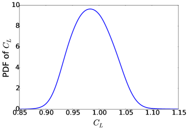
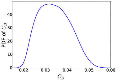
Fig. 8 presents the statistics for a Latin Hypercube sampling of the PCE surrogate with $10^{6}$ samples. This surrogate required 1,103 flow solver evaluations to converge, which is reasonable for a 5 dimensional parameter space. Convergence is based on the change in the $L_{2}$ norm of the surrogate response covariance matrix falling below some threshold (which we set to be equal to $10^{-4}$).

The first thing to note is that we can easily see that $C_{L}$ and $C_{D}$ correlate very strongly (corr$(C_{L},C_{D})=-0.94$), which indicates that over our parameter range, we only need to examine one of the two in order to understand the effects of our inputs on aerodynamic performance.

In order to examine the independent relative contributions of each of our 5 input parameters to the variance of our responses, we examine both the data correlations and the Sobol indices (defined previously in Eq. (8)). Loosely speaking, the Sobol index gives a measure of how much, on average, a parameter (or a combination of parameters) contributes to the total variance of the response. It is clear from these metrics that variations in horn position, $b$, contribute the most to the variance of our response and hence $b$ is the “most important” parameter. The caveat of this statement, of course, is that it only applies over the limited parameter range we have chosen. Had we chosen to investigate larger variations in height, for example, then height could very well be the dominant parameter.

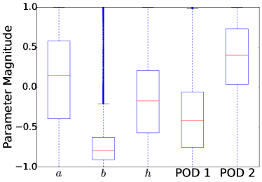
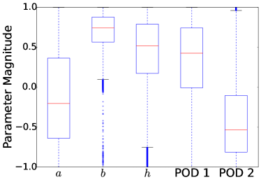
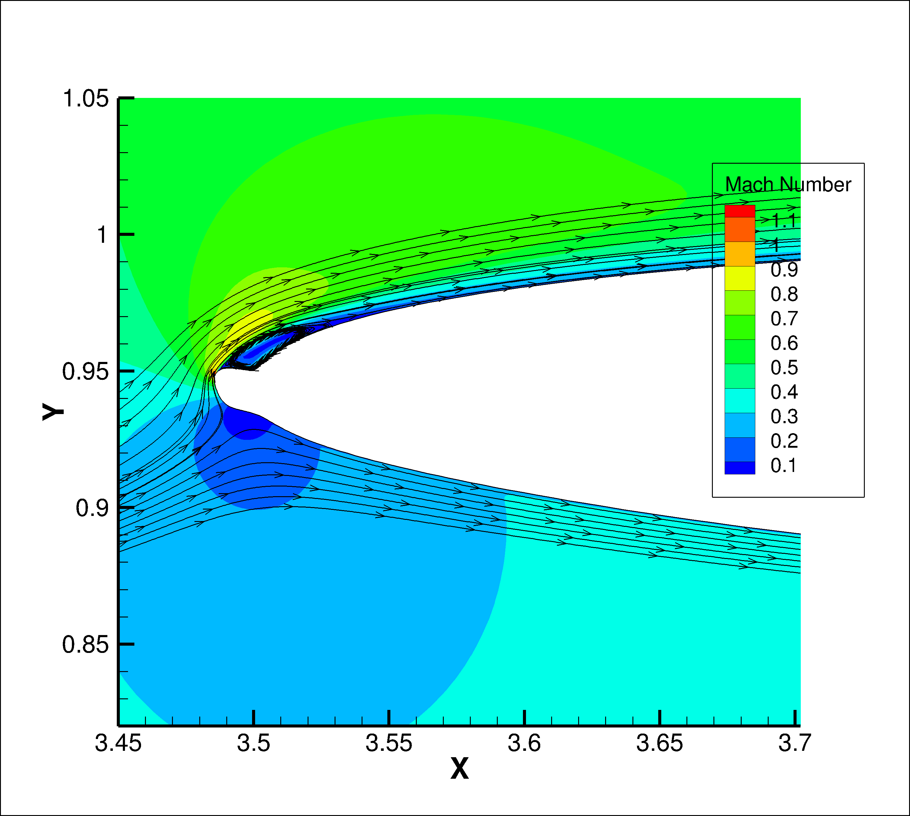
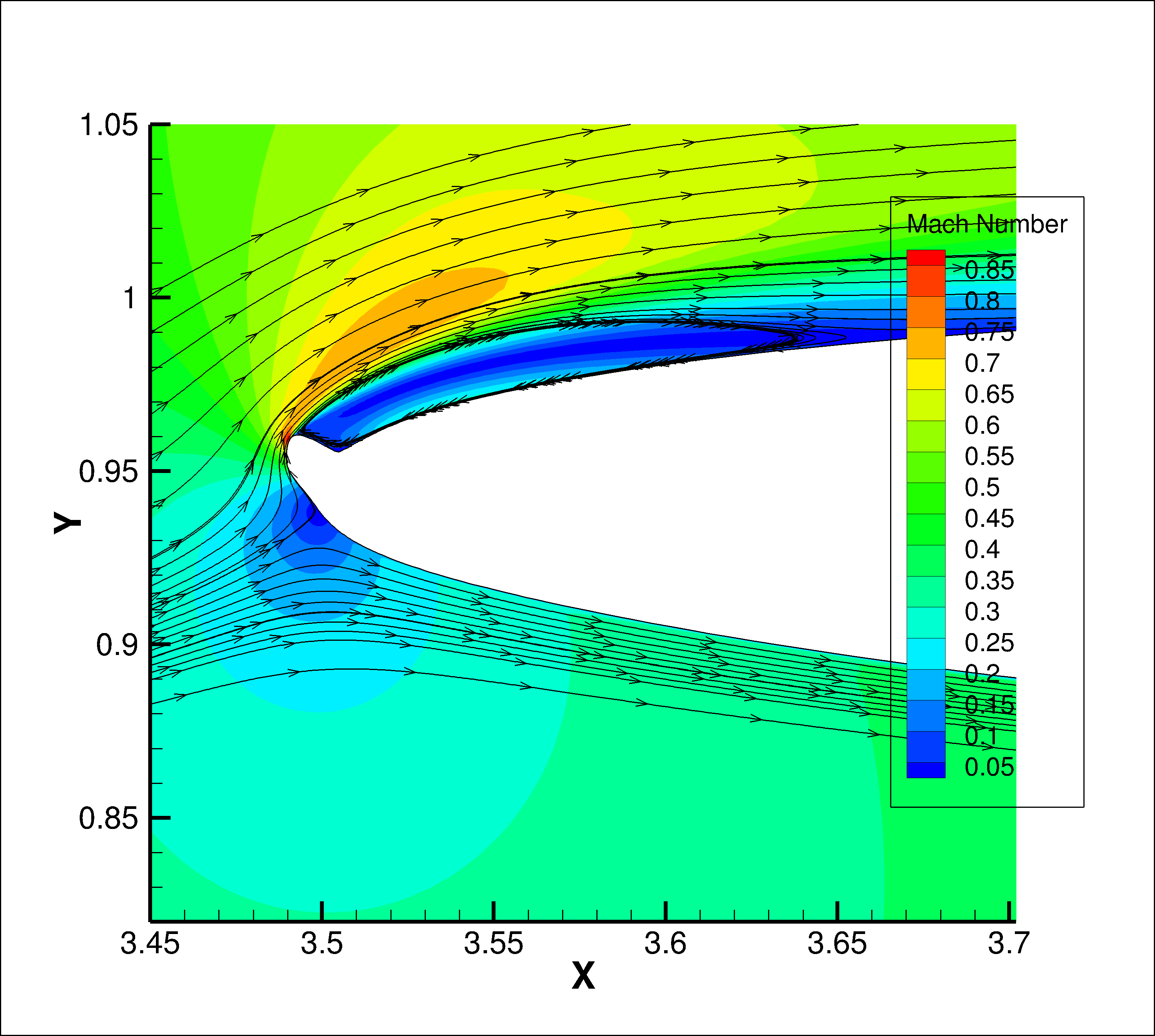
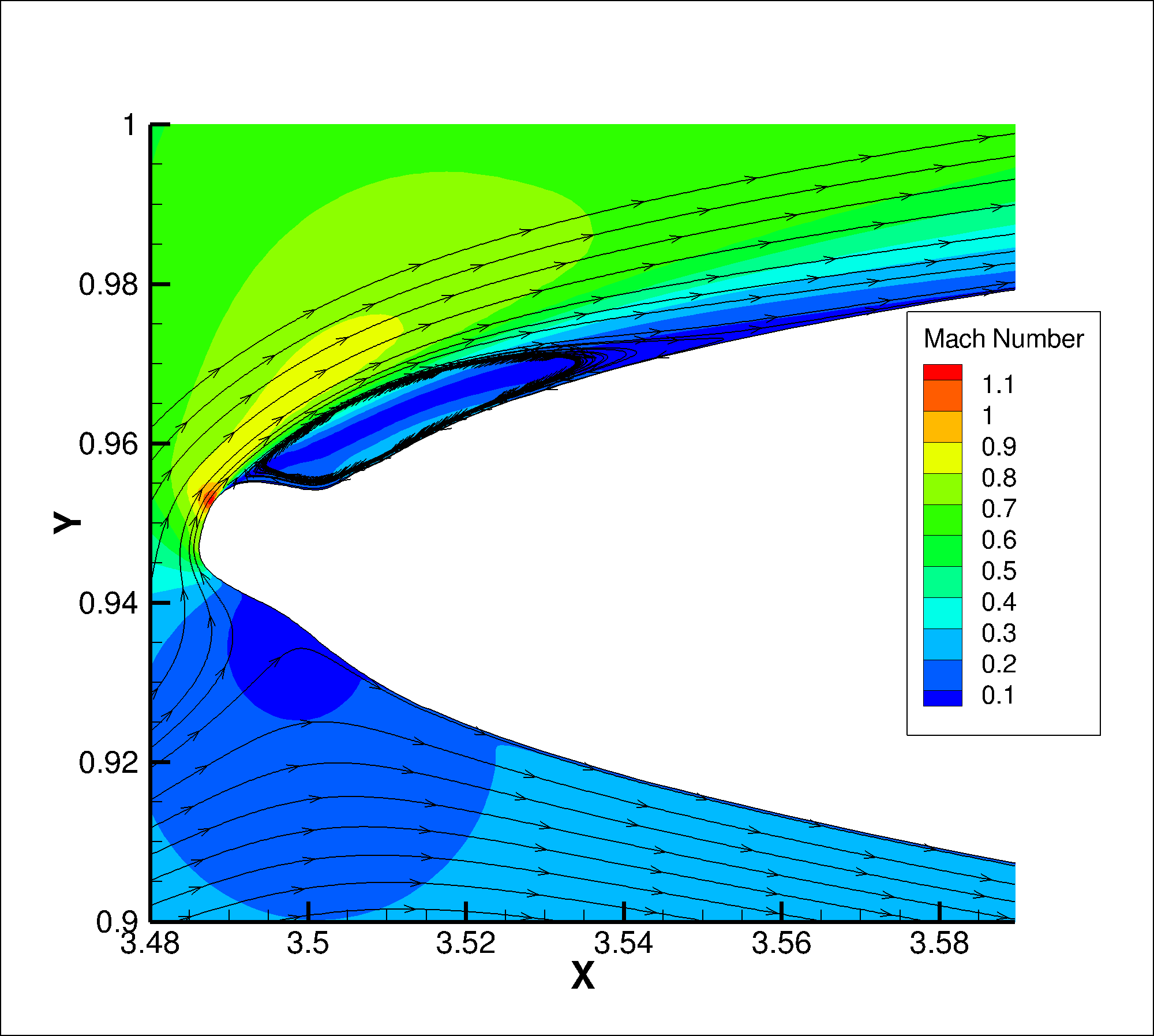
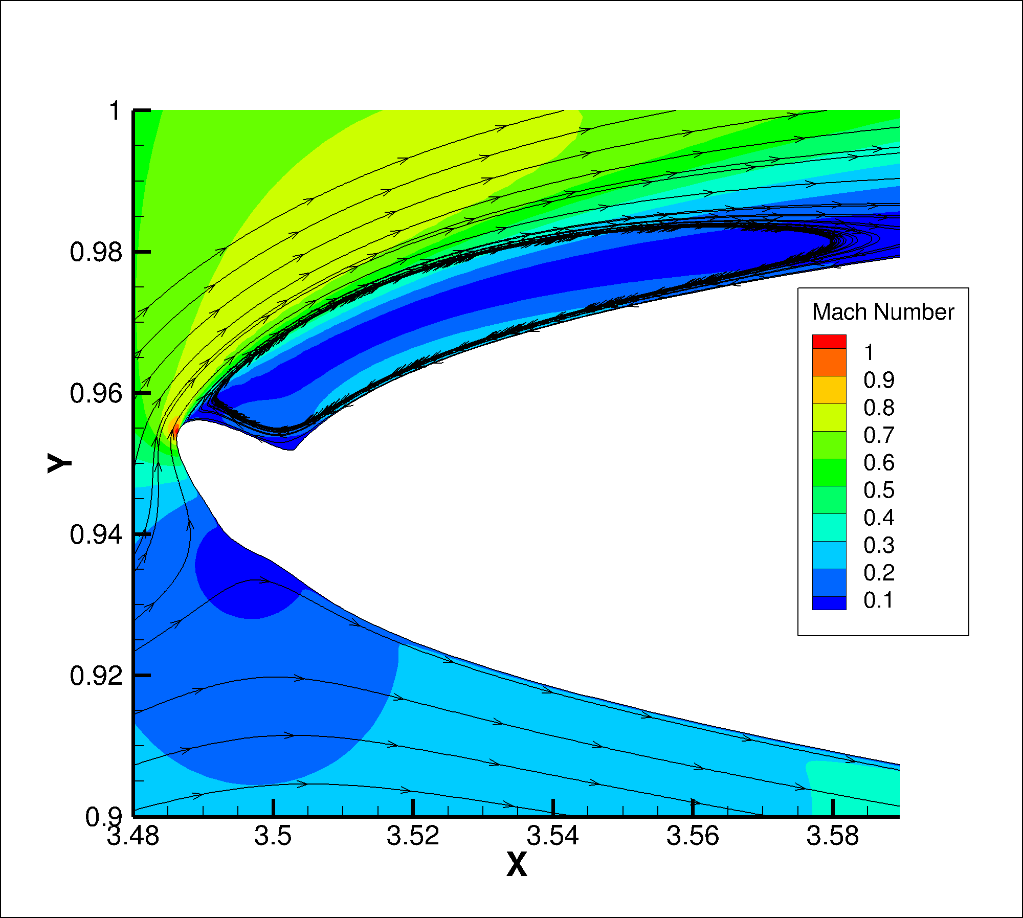
The sign of the correlation of horn position with our responses indicates that performance degrades (ie., lower lift, higher drag) as the horn moves closer to the upper surface. The physical explanation for this is intuitive, and can ascertained by inspecting Fig. 10. The upper surface horn is a more obtrusive flow obstacle, and therefore promotes a larger steady-state separation bubble aft of the horn than the equally-sized (but less obtrusive) lower horn. This phenomenon agrees with similar findings in a related study [2].

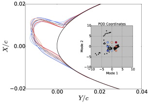
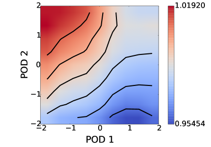
Although horn position is the most dominant parameter, the other parameters do affect performance; this can be revealed by examining the correlations in Table 1. As expected, taller horns give worse performance than shorter ones. Performance is relatively insensitive to variations in width, but there is a slight tendency for narrower horns to give worse performance than wider horns. This is because narrower horns come to a sharper point and hence promote larger leading edge separation bubbles, whereas wider horns have more rounded points and hence are less severe. Perhaps not as immediately clear is the effect of the POD modes on performance. One way to gain some insight into this is to project the surrogate onto the two-parameter space of POD coefficients. This can be approximated by sampling the surrogate, and then locally averaging out the three scaling parameters. This produces Fig. 11, which demonstrates that the POD modes can interact in such a way as to produce a distinct skew to the horn. Depending on the direction of this skew, this can either help or hurt aerodynamic performance, since the length of the leading edge separation bubble depends on the horn shape details.

Integrating all of these analyses together gives a clean, intuitive picture of the effects of our 5 parameters on the flow. We find that the “worst” horn shapes in our parameter space are tall, narrow, upper surface horns that have a sharp upper skew shape; the “best” ones are short, wide and rounded, located on the lower surface, and have gentle downward skew (or no skew at all). This is affirmed by examining Fig 9, which shows clear statistical clustering of the horn shapes in parameter space that produce the best and worst aerodynamic performance.

(a) Favorable horns.

(b) Unfavorable horns.

Figure 9: Statistical clustering of “good” (bottom 10$\%$ of $C_{L}$) and “bad” (top 10$\%$ of $C_{L}$) horns in parameter space, based on $10^{6}$ Latin Hypercube samples of the surrogate. The parameter magnitudes have all been linearly scaled to lie between $\pm 1$.

(a) Lower surface horn.

(b) Upper surface horn.

Figure 10: Flow field contours (of Mach number) for two horns of equal size and shape that differ only in their relative positions. The horn in ($b$) is more normal to the freestream flow than the horn in ($a$), and hence generates a larger scale leading edge separation bubble.

(a) Favorably skewed horn.

(b) Unfavorably skewed horn.

(c) Contours of $\mathbb{E}(C_{L}|\text{POD1, POD2})$

Figure 11: Effect of POD coefficients on performance. Part ($c$) displays contours of $C_{L}$ as a function of the POD coefficients, obtained by sampling the PCE surrogate and locally averaging over $b$ and $h$. Parts ($a$-$b$) display two horns that are the same size/position, but differ in their POD coefficients. This gives rise to favorable/unfavorable skewness in the shape.

4 Results: Ice Shapes from Wind Tunnel Experiments

Our goal in the preceding example was to use a dataset in which the individual ice shapes exhibited only modest variation from the mean shape. This ensured that we could obtain a faithful representation of the ice using only a modest number of parameters (five). In this section, we are interested in applying the same techniques to a dataset whose entries represent a much wider range of physical conditions, and hence a much wider range of shapes. As we will see, doing this comes at the cost of having to retain more POD modes to accurately represent the ice, which translates into a much larger UQ study.

Two resources that provide an excellent sampling of 2D ice shapes for different airfoil geometries subjected to different icing conditions are Addy [15], and Wright and Rutkowski [16]. For the studies used in this example, we use a subset of the shapes found in Addy. The shapes found in this database were generated in a wind tunnel by exposing different airfoils to a wide range of icing conditions. The conditions used reflect the guidelines and standards for atmospheric icing conditions as defined by the Federal Aviation Administration (Federal Aviation Regulations 25 Appendix C). In that database, three clean airfoil geometries are used – one which represents a business jet, one which represents a commercial transport, and one which represents a general aviation aircraft.

In this example, we limit the entries of our dataset to the business jet ice shapes. We do this because having several different clean airfoil geometries in our dataset would complicate our POD data reduction, since in that case, one would not be able to uniformly define the demarcations between the template (ie. the clean airfoil) and the ice/air for all entries. Similarly, it would also make unclear the choice of clean airfoil to use when generating artificial ice shapes based on the POD modes. Consideration of the remaining two datasets in Addy (the commercial transport and the general aviation aircraft) would certainly make for interesting parallel studies, however, we leave this as an item to be addressed in future work.

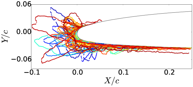
There were 54 total shapes from the business jet dataset. A plot of all of these shapes together on the same airfoil is shown in Fig. 12. As can be observed, there is significant variation in the size and shape details of the ice. These shapes were generated from variations in the following range of icing conditions:

• Mach number $\in[0.28,0.39]$

• Airspeed $\in[175,250]$ knots

• Attitude $\in[1.5,6.0]^{\circ}$

• Free-stream temperature $\in[-27.8,-0.7]^{\circ}C$

• Surface temperature $\in[-31.6,-5.0]^{\circ}C$

• MVD $\in[15,160]\mu m$

• LWC $\in[0.310,1.6]\frac{g}{m^{3}}$

• Exposure time $\in[0.7,45]$ min

See Addy [15] (pg. 40) for further details.

Figure 12: Ice shape dataset, from Addy[15]. $c$ denotes the chord (set to 1 in all examples).

4.1 POD of the Ice Shape Data

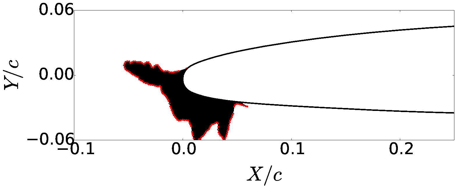
In order to apply the methods above to our ice shape problem, we need to first determine an appropriate vector space representation of the ice shapes. There is not necessarily one unique way of doing this. We approach this problem by finding a rectangular window of space in which all of the ice shapes in Fig. 12 fit, and overlaying this space with a static Cartesian mesh. For a particular ice shape, we assign a value of 1 to a particular grid point if that grid point is inside/on the body of the ice, or a value of 0 if it is not. It should be noted that any points inside the clean airfoil were excepted from the grid, so that our mesh consists entirely of points located either in the free-stream, or in the ice. The background mesh consists of roughly $N=7\times 10^{5}$ points. An example of this process is shown in Fig. 13.

Figure 13: Illustration of how ice shapes are defined for POD. Each ice shape is defined on a static Cartesian background mesh, the bounds of which form the rectangular window of this figure. For a particular ice shape, a grid point is assigned a value of 1 if that point is located inside the ice boundary. The ice boundary is shown in dotted red; points on the ice are shown in dotted black.

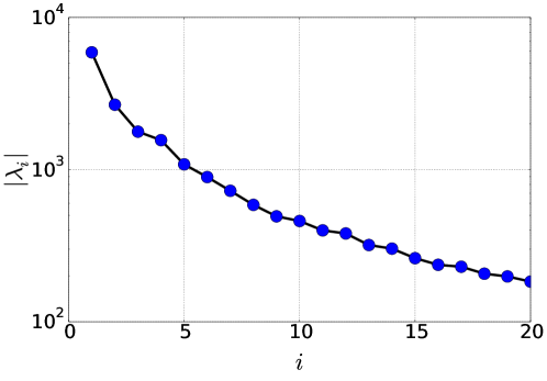
Having cast all of our ice shapes in the same $N$-dimensional vector space, we are now in a position to compute the POD modes. Because we will ultimately be doing UQ on the POD modes, we would like to retain as few modes as possible while still having accurate representation power in that basis. This is the classic tradeoff between economy and accuracy in low-dimensional modeling. In order to make an informed decision on how many modes to keep, we look at the magnitude of the POD eigenvalues, shown in Fig. 14.

We make the decision to truncate the expansion at order 8, where the magnitudes of the eigenvalues have decayed by about one order of magnitude. Retaining more modes would present a more computationally laborious UQ study. Additionally – as we will demonstrate shortly – projection of the original dataset onto the first 8 modes yields good reconstructions, so higher order modes may be practically unnecessary.

The mean and leading POD modes are shown in Fig. 15. As can be seen, the mean and lowest order modes have the most effect on the underside of the airfoil, where – in our dataset – there is a high probability of having ice (many of our ice shapes have “tails” on the airfoil underside). The higher order modes appear to be critical to attaining the extreme shapes in our dataset. Intuitively, we might expect these modes to have a more significant impact on the aerodynamics than the lower order ones.

Figure 14: Magnitudes of the POD eigenvalues.

2

(a) Mean

(b) Mode 1

(c) Mode 2

(d) Mode 3

(e) Mode 4

(f) Mode 5

Figure 15: Mean and POD Modes.

4.2 POD Reconstructions of the Ice Shapes

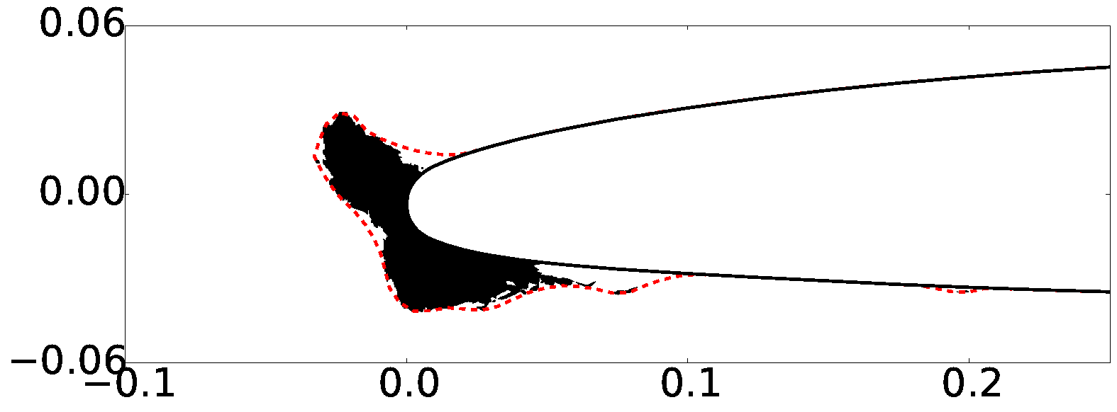
We can now investigate how faithful our reconstructions of the original dataset are using our POD basis. It is important to realize that our POD reconstructions will need to be filtered a posteriori. This is because the reconstructions will, in general, consist of grid point values that are between 0 and 1. However, our ice shapes are binary in nature – a particular grid point should either be 1 if it is on the ice, or 0 if it is not.

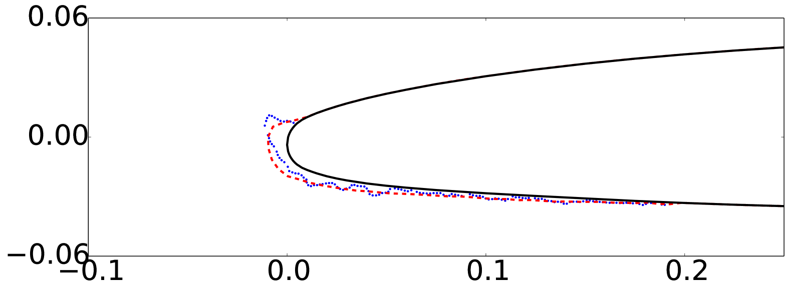
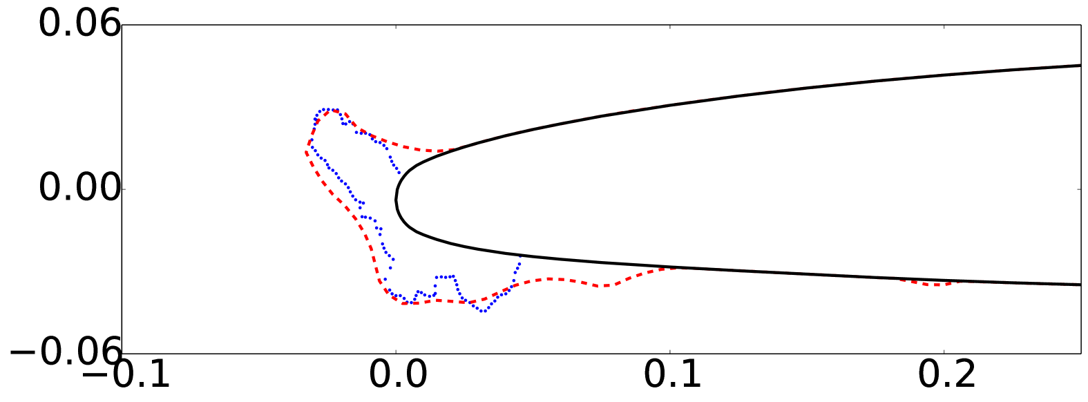
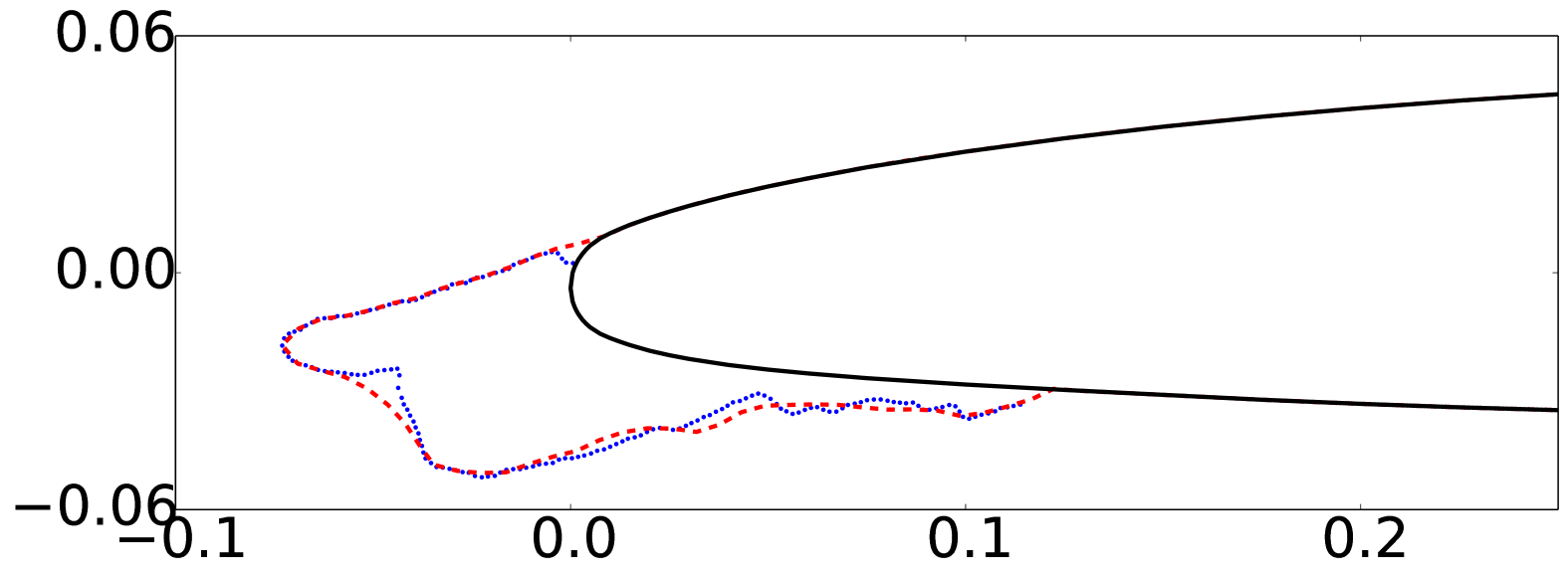
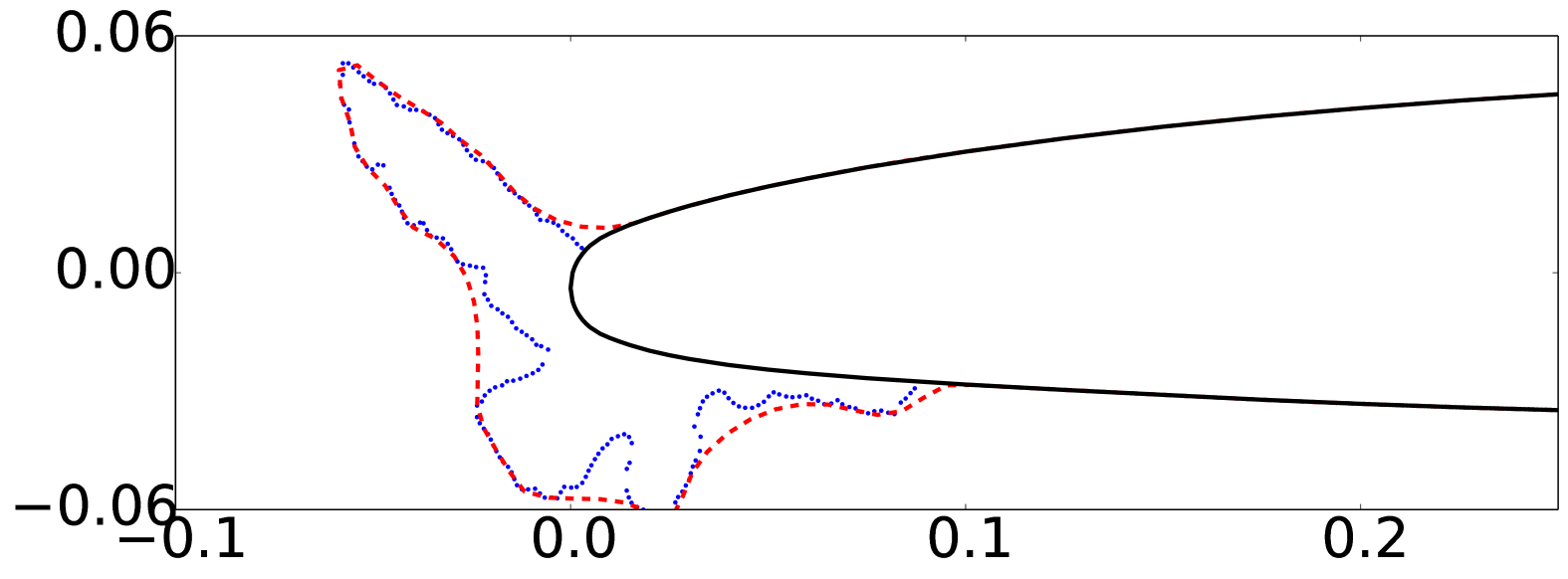
To rectify this issue, we use a simple filter that rounds everything less than 0.5 to 0, and everything greater than 0.5 to 1. An example of this procedure is shown in Fig. 16. Several filtered reconstructions are shown in Fig. 17. As can be seen, the reconstructions are of satisfactory agreement with the original data, which reaffirms our choice of truncating the expansion at 8 modes.

2

(a) Unfiltered reconstruction

(b) Filtered reconstruction

Figure 16: Unfiltered (a) and filtered (b) projections of an ice shape from the dataset onto the POD basis.

2

Figure 17: Original data (blue) compared to reconstructions (red) using 8 POD modes.

4.3 Airfoil Icing UQ: 8 Parameter Scenario

The final step in this study is to apply the UQ techniques that we have used in the previous example to this scenario, in which we have an 8-dimensional parameter space that consists of variations of our POD coefficients. Based on how many evaluations were required for the 5-parameter UQ study, we estimate that this UQ study may require somewhere between five and ten-thousand flow solver evaluations to yield a converged, faithful PCE surrogate. These simulations require two to four weeks of wall-clock time, and are currently underway. We will report the results when they become available.

5 Conclusions

Wing icing is not only dangerous to pilots, it is a complex physics problem that is subject to a large amount of uncertainty. Quantifying the exact effects of this uncertainty on airplane performance is hence of great importance to airplane safety.

The purpose of this paper within that context is twofold: to introduce a framework for low-dimensional modeling and data reduction for ice shape datasets, and to introduce a fast, accurate, and efficient means for quantifying uncertainty in the resulting shape parameter spaces. Towards this end, we analyzed two examples, one in which the dataset came from 2D spanwise cross-sections of a 3D wing icing computation, and one in which the dataset came from icing wind tunnel experiments performed at a wide range of icing conditions. In the first example, we were able to effectively model the dataset using only 5 parameters, successfully create a PCE surrogate, and analyze the surrogate statistics for insights into the fundamental physics of how the horn affects the aerodynamics. The second example is demonstrative of how one can model more complicated ice shapes. In that example, we were able to model the ice shape dataset, but required 8 parameters to do so.

Much work and research remains to be done on these subjects in the future. To begin, we need to complete our 8-parameter UQ study, which will help enrich our understanding of the effects of more exotic ice shapes on airfoil aerodynamics. Another possible avenue for research is to first classify ice shapes into several distinct categories (based on similarity in shape, similarity in the physical conditions used to generate the shapes, etc.), and then to perform POD/UQ separately on each of these classes. This approach would help alleviate the curse of dimensionality, by reducing the number of parameters in each class.

References

- [1] Landsberg, B., “Aircraft Icing,” Safety Advisor, Weather No. 1, Aircraft Owners and Pilots Association Air Safety Foundation, 2002.
- [2] DeGennaro, A., Rowley, C. W., and Martinelli, L., “Uncertainty Quantification for Airfoil Icing using Polynomial Chaos Expansions,” To appear in Journal of Aircraft, 2015.
- [3] Holmes, P., Lumley, J., Berkooz, G., and Rowley, C., Turbulence, Coherent Structures, Dynamical Systems and Symmetry, Cambridge University Press, New York, 2012.
- [4] Martinelli, L. and Jameson, A., “Validation of a Multigrid Method for the Reynolds Averaged Equations,” AIAA paper 88-0414, 1988.
- [5] Tatsumi, S., Martinelli, L., and Jameson, A., “A New High Resolution Scheme for Compressible Viscous Flows with Shocks,” AIAA paper 95-0466, Jan. 1995.
- [6] Tatsumi, S., Martinelli, L., and Jameson, A., “Flux Limited Schemes for the Compressible Navier-Stokes Equations,” AIAA Journal, Vol. 33, No. 2, 1995, pp. 252–261.
- [7] Spalart, P. and Allmaras, S., “A One-Equation Turbulent Model for Aerodynamic Flows,” AIAA Paper 92-0439, 30th AIAA Aerospace Sciences Meeting, Reno, NV, Jan. 1992.
- [8] Ghanem, R. G. and Spanos, P., Stochastic Finite Elements: A Spectral Approach, Springer-Verlag, New York, 1991.
- [9] Xiu, D., Numerical Methods for Stochastic Computations: A Spectral Method Approach, Princeton University Press, 2010.
- [10] LeMaitre, O., Spectral Methods for Uncertainty Quantification, Springer, 2010.
- [11] Smolyak, S. A., “Quadrature and Interpolation Formulas for Tensor Products of Certain Classes of Functions,” Soviet Math. Dokl., Vol. 4, 1963, pp. 240–243.
- [12] Gerstner, T. and Griebel, M., “Numerical Integration using Sparse Grids,” Numerical Algorithms, Vol. 18, 1998, pp. 209–232.
- [13] Adams, B. M., Bohnhoff, W. J., Dalbey, K. R., Eddy, J. P., Eldred, M. S., Gay, D. M., Haskell, K., Hough, P. D., and Swiler, L. P., “DAKOTA, A Multilevel Parallel Object-Oriented Framework for Design Optimization, Parameter Estimation, Uncertainty Quantification, and Sensitivity Analysis: Version 5.3 User’s Manual,” Sandia Technical Report SAND2010-2183, 2013.
- [14] Broeren, A., Potapczuk, M., Riley, J., Villedieu, P., Moens, F., and Bragg, M., “Swept-Wing Ice Accretion Characterization and Aerodynamics,” AIAA Paper 2013-2824, 2013.
- [15] Addy, H. E., “Ice Accretions and Icing Effects for Modern Airfoils,” Tech. Rep. TP 2000-210031, NASA, April 2000.
- [16] Wright, W. B. and Rutkowski, A., “Validation Results for LEWICE 2.0,” Tech. Rep. CR 1999-208690, NASA, Jan. 1999.