Visual sphere and Thurston’s boundary of the Universal Teichmüller space

Abstract.

Thurston’s boundary to the universal Teichmüller space $T(\mathbb{D})$ is the space $PML_{bdd}(\mathbb{D})$ of projective bounded measured laminations of $\mathbb{D}$. A geodesic ray in $T(\mathbb{D})$ is of Teichmüller type if it shrinks vertical foliation of an integrable holomorphic quadratic differential. In a prior work we established that each Teichmüller geodesic ray limits to a multiple (by the reciprocal of the length of the leaves) of vertical foliation of the quadratic differential.

Certain non-integrable holomorphic quadratic differential induce geodesic rays and we consider their limit points in $PML_{bdd}(\mathbb{D})$. Somewhat surprisingly, the support of the limiting projective measured laminations might be a geodesic lamination whose leaves are not homotopic to leaves of either vertical or horizontal foliation of the non-integrable holomorphic quadratic differential.

1. Introduction

Let $\mathbb{D}$ be the unit disk model of the hyperbolic plane. The Teichmüller space $T(\mathbb{D})$ of the hyperbolic plane $\mathbb{D}$, called the universal Teichmüller space, consists of all quasisymmetric maps $h:S^{1}\to S^{1}$ which fix $1$, $i$ and $-1$ (cf. [5]). The Teichmüller space of an arbitrary hyperbolic surface embeds in $T(\mathbb{D})$ as a complex Banach submanifold. Thurston’s boundary to the universal Teichmüller space $T(\mathbb{D})$ is the space $PML_{bdd}(\mathbb{D})$ of projective bounded measured laminations of $\mathbb{D}$ (cf. [20], [22]). Teichmüller geodesic rays are obtained by shrinking vertical trajectories of integrable holomorphic quadratic differentials. A Teichmüller geodesic ray corresponding to an integrable holomorphic quadratic differential $\varphi$ limits to a unique point in Thurston’s boundary whose support geodesic lamination is homotopic to vertical foliation of $\varphi$ and the transverse measure is given by integrating the reciprocal of the lengths of vertical leaves against $Re(\sqrt{\varphi dz^{2}})$ (cf. [9]). Certain non-integrable holomorphic quadratic differentials induce geodesic rays in $T(\mathbb{D})$ by shrinking their vertical trajectories in the same fashion as for integrable differentials. We study the limits of these geodesic rays on Thurston’s boundary to $T(\mathbb{D})$.

The space $G(\mathbb{D})$ of oriented geodesics of $\mathbb{D}$ is identified with $S^{1}\times S^{1}-diag$ since each geodesic is uniquely determined by the ordered pair of its ideal endpoints on $S^{1}$. A geodesic current is a positive Borel measure on $G(\mathbb{D})$. The universal Teichmüller space $T(\mathbb{D})$ embeds into the space of geodesic currents when equipped with the uniform weak* topology (cf. [22]). Thurston’s boundary to $T(\mathbb{D})$ is the set of asymptotic rays to the image of $T(\mathbb{D})$ in the space of geodesic currents and it is identified with the space $PML_{bdd}(\mathbb{D})$ of projective bounded measured laminations of $\mathbb{D}$ (cf. [22]). This approach was first introduced by Bonahon [3] to give an alternative description of Thurston’s boundary of the Teichmüller space $T(S)$ of a closed surface $S$ of genus at least two.

In the case of closed surfaces, Masur [15] proved that Teichmüller geodesic rays obtained by shrinking vertical trajectories of holomorphic quadratic differentials with uniquely ergodic vertical foliations converge to the projective classes of their vertical foliations in Thurston’s boundary. However, when vertical foliations of holomorphic quadratic differentials on closed surfaces are not uniquely ergodic then the limit sets of the corresponding Teichmüller geodesic rays consist of more than one point while their supports are homotopic to vertical foliation of the quadratic differential (cf. [14], [13]). On the other hand, the limits of Teichmüller geodesic rays in the universal Teichmüller space $T(\mathbb{D})$ corresponding to integrable holomorphic quadratic differentials always have a unique endpoint in Thurston’s boundary of $T(\mathbb{D})$ (cf. [9]).

Let $\varphi$ be an integrable holomorphic quadratic differential on $\mathbb{D}$. Each vertical trajectory of $\varphi$ has two distinct endpoints on the boundary circle $S^{1}$ of the hyperbolic plane $\mathbb{D}$ (cf. [23]). Thus each vertical trajectory of $\varphi$ is homotopic to a unique geodesic of $\mathbb{D}$ relative ideal endpoints on $S^{1}$. Let $v_{\varphi}$ be the set of the geodesics in $\mathbb{D}$ homotopic to the vertical trajectories of $\varphi$. Given a box of geodesics $[a,b]\times[c,d]\subset S^{1}\times S^{1}-diag$, denote by $I_{[a,b]\times[c,d]}$ (at most countable) union of sub-arcs of horizontal trajectories that intersects exactly once each vertical trajectory of $\varphi$ with one endpoint in $[a,b]$ and the other endpoint in $[c,d]$, and that does not intersect any other vertical trajectories of $\varphi$.

Define measured laminations $\nu_{\varphi}$ and $\mu_{\varphi}$ of $\mathbb{D}$ supported on $v_{\varphi}$ by

$$\nu_{\varphi}([a,b]\times[c,d])=\int_{I_{[a,b]\times[c,d]}}dx$$

and

$$\mu_{\varphi}([a,b]\times[c,d])=\int_{I_{[a,b]\times[c,d]}}\frac{1}{l(x)}dx$$

where $x=\int_{*}\sqrt{\varphi}dz$ is the natural parameter of $\varphi$ and $l(x)$ is the $\varphi$-length of the vertical trajectory through $x$ (cf. [9]). Then (cf. [9])

$$\epsilon T_{\epsilon}\to\mu_{\varphi}$$

as $\epsilon\to 0^{+}$ in the weak* topology on geodesic currents, where $T_{\epsilon}$ is a quasiconformal map of $\mathbb{D}$ that shrinks the vertical trajectories of $\varphi$ by a multiplicative constant $\epsilon$. In other words, the Teichmüller geodesic ray $T_{\epsilon}$ converges to $[\mu_{\varphi}]\in PML_{bdd}(\mathbb{D})$.

The space of all geodesic rays in the Teichmüller metric starting at the basepoint $[id]\in T(\mathbb{D})$ leaving every bounded subset of $T(\mathbb{D})$ is called the visual boundary of the universal Teichmüller space $T(\mathbb{D})$. The Teichmüller geodesic rays-obtained by shrinking the vertical direction of an integrable holomorphic quadratic differential $\varphi$-form an open and dense subset of $T(\mathbb{D})$ (cf. [5]). However, there exist geodesic rays different from Teichmüller geodesic rays. A Beltrami coefficient $\xi$ of a quasiconformal map $f:\mathbb{D}\to\mathbb{D}$ is said to be extremal if $\|\xi\|_{\infty}$ is minimal among all Beltrami coefficients of quasiconformal maps representing the same point in $T(\mathbb{D})$ (where $f,g:\mathbb{D}\to\mathbb{D}$ represent the same point of $T(\mathbb{D})$ if $f|_{S^{1}}=g|_{S^{1}}$ [5]). If an extremal Beltrami coefficient $\xi$ is not of the Teichmüller type $k\frac{|\varphi|}{\varphi}$ for $0<k<1$ and $\varphi$ integrable, then $t\mapsto t\xi$ for $t\in[0,\frac{1}{\|\xi\|_{\infty}})$ is a geodesic ray that is not a Teichmüller geodesic ray.

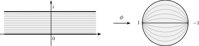
Figure 1. Horizontal strip $S$ and its Riemann map. The dotted lines represent the horizontal trajectories of the standard quadratic differential $dz^{2}$ in $S$ and their images in $\mathbb{D}$ under $\phi$.

We consider the limits of two (non-Teichmüller) geodesic rays introduced by Strebel [5]. The first example is given by a horizontal strip $S=\{0<Im(z)<1\}$ with the Beltrami coefficient $\xi=k\frac{|\varphi|}{\varphi}$ with $\varphi(z)\equiv 1$. Since $S$ does not have finite Euclidean area, the holomorphic quadratic differential $\varphi$ is not integrable and the corresponding geodesic ray is not Teichmüller. Note that $S$ is conformally identified with $\mathbb{D}$ and this identification is implicitly assumed. We denote by $T_{\epsilon}$ the shrinking of vertical trajectories by the factor $\epsilon$ and denote by $T_{1/\epsilon}$ the stretching of the vertical trajectories of $\varphi$ by the factor $1/\epsilon$ as $\epsilon\to 0^{+}$. We prove (cf. Theorem 4.1 and Figure 1)

Theorem 1. Let $S=\{0<Im(z)<1\}$ be a horizontal strip and let $\varphi(z)=1$ for all $z\in S$. Denote by $T_{\epsilon}$, $\epsilon>0$, the geodesic ray in $T(\mathbb{D})$ obtained by shrinking the vertical leaves of $\varphi$ by a factor $\epsilon$ and denote by $T_{\frac{1}{\epsilon}}$, $\epsilon>0$, the geodesic ray in $T(\mathbb{D})$ obtained by stretching the vertical leaves by a factor $\frac{1}{\epsilon}$.

Let $\nu_{1}$ be the (hyperbolic) measured lamination on $S$ whose support is homotopic to the vertical foliation of $\varphi(z)=1$ on $S$ and whose transverse measure is given by the euclidean length of the transverse horizontal set. Let $\nu_{2}$ be the dirac measured lamination on $S$ with support the hyperbolic geodesic homotopic to horizontal trajectories in $S$.

Then we have

$$T_{\epsilon}\to[\nu_{1}]$$

and

$$T_{1/\epsilon}\to[\nu_{2}]$$

as $\epsilon\to 0^{+}$ in Thuston’s boundary $PML_{bdd}(\mathbb{D})$ of the universal Teichmüller space $T(\mathbb{D})$. The rate of convergence of $T_{\epsilon}$ is $1/\epsilon$ and the rate of convergence of $T_{1/\epsilon}$ is $1/\epsilon^{*}$, where $\epsilon^{*}\to 0^{+}$ as $\epsilon\to 0^{+}$.

Remark 1. Note that all vertical trajectories in $S$ have finite $\varphi$-lengths which is the same as in the case of integrable holomorphic quadratic differentials. On the other hand, horizontal trajectories of $\varphi$ have infinite lengths. Unlike for intergrable case, this makes the $\varphi$-metric unsuitable for making allowable metrics when computing moduli of various quadrilaterals and we find a new method for dealing with the difficulty.

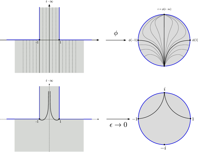
Figure 2. Strebel’s chimney domain and its Riemann map. The dotted lines represent the vertical trajectories of the standard quadratic differential $dz^{2}$ in $C$ and their images in $\mathbb{D}$ under $\phi$.

Next we consider Strebel’s chimney domain $C=\{z:Im(z)<0\}\cup\{z:|Re(z)|<1\}$. The holomorphic quadratic differential $\varphi(z)dz^{2}=dz^{2}$ is not integrable on $C$ while the corresponding Beltrami coefficient $k\frac{|\varphi|}{\varphi}=k$ is extremal. Denote by $T_{\epsilon}$ as $\epsilon\to 0^{+}$ the geodesic ray obtained by shrinking the vertical foliation of $\varphi$ by the factor $\epsilon$. We prove (cf. Theorem 4.3 and Figure 2)

Theorem 2. Let $\nu$ be a measured lamination on $C$ which is a sum of two Dirac measured laminations supported on geodesics $\gamma_{1}$ and $\gamma_{2}$ in $C$ with endpoints $1,+\infty\in\partial C$ and endpoints $-1,+\infty\in\partial C$, respectively. Then

$$T_{\epsilon}\to[\nu]$$

as $\epsilon\to 0^{+}$ in Thuston’s closure $T(\mathbb{D})\cup PML_{bdd}(\mathbb{D})$ of the universal Teichmüller space $T(\mathbb{D})$. The rate of convergence of $T_{\epsilon}$ is $1/\epsilon^{*}$, where $\epsilon^{*}\to 0^{+}$ as $\epsilon\to 0^{+}$.

Remark 2. All vertical leaves on $C$ have infinite lengths. If vertical leaves are straightened into hyperbolic geodesics, then the geodesic lamination $v_{\varphi}$ does not contain $g_{1}$ and $g_{2}$ even in its closure. Therefore it is impossible to detect $g_{1}$ and $g_{2}$ just by $v_{\varphi}$ alone. In fact, the limits $g_{1}$ and $g_{2}$ appear due to the fact that vertical trajectories accumulate to parts of the boundary of $C$.

2. Thurston’s boundary via geodesic currents

We identify the hyperbolic plane with its upper half-plane model $\mathbb{D}$; the visual boundary $S^{1}=\mathbb{R}\cup\{\infty\}$ to $\mathbb{D}$ is homeomorphic to the unit circle. An orientation preserving homeomorphism $h:S^{1}\to S^{1}$ is said to be quasisymmetric if there exists $M\geq 1$ such that

$$\frac{1}{M}\leq\frac{|h(e^{x+t})-h(e^{x})|}{|h(e^{x})-h(e^{x-t})|}\leq M$$

for all $x\in\mathbb{R}$ and $t>0$. A homeomorphism is quasisymmetric if and only if it extends to a quasiconformal map of the unit disk.

Definition 2.1.

The universal Teichmüller space $T(\mathbb{D})$ consists of all quasisymmetric maps $h:S^{1}\to S^{1}$ that fix $1,i,-1\in S^{1}$.

If $g:\mathbb{D}\to\mathbb{D}$ is a quasiconformal map, denote by $K(g)$ its quasiconformal constant. The Teichmüller metric on $T(\mathbb{D})$ is given by $d(h_{1},h_{2})=\inf_{g}K(g)$, where $g$ runs over all quasiconformal extensions of the quasisymmetric map $h_{1}\circ h_{2}^{-1}$. The Teichmüller topology is induced by the Teichmüller metric.

The space $G(\mathbb{D})$ of oriented geodesics on $\mathbb{D}$ is identified with $S^{1}\times S^{1}-diag$. A geodesic current is a Borel measure on $G(\mathbb{D})$. The Liouville measure $\mathcal{L}$ on the space of geodesic of $\mathbb{D}$ is given by

$$\mathcal{L}(A)=\int_{A}\frac{|dx||dy|}{|x-y|^{2}}$$

for any Borel set $A\subset S^{1}\times S^{1}-diag$. If $A=[a,b]\times[c,d]$ is a box of geodesic then

$$\mathcal{L}([a,b]\times[c,d])=\log\frac{(a-c)(b-d)}{(a-d)(b-c)}.$$

The universal Teichmüller space $T(\mathbb{D})$ maps into the space of geodesic currents by taking the pull backs by quasisymmetric maps of the Liouville measure. A geodesic current $\alpha$ is bounded if

$$\sup_{[a,b]\times[c,d]}\alpha([a,b]\times[c,d])<\infty$$

where the supremum is over all boxes of geodesics $[a,b]\times[c,d]$ with $\mathcal{L}([a,b]\times[c,d])=\log 2$. The pull backs $h^{*}(\mathcal{L})$ for $h$ quasisymmetric are bounded geodesic currents (cf. [20]).

The pull backs of the Liouville measure define a homeomorphism of $T(\mathbb{D})$ onto its image in the bounded geodesic currents, when the space of geodesic currents is equipped with the uniform weak* topology ([22]). The asymptotic rays to the image of $T(\mathbb{D})$ are identified with the space of projective bounded measured laminations (cf. [22], [20]). Thus Thurston’s boundary of $T(\mathbb{D})$ is the space $PML_{bdd}(\mathbb{D})$ of all projective bounded measured laminations on $\mathbb{D}$ (and an analogous statement holds for any hyperbolic Riemann surface). Bonahon [3] introduced this approach for closed surfaces in order to give an alternative definition of Thurston’s boundary.

3. The asymptotics of the modulus

Let $(a,b,c,d)$ be a quadruple of distinct points on $S^{1}$ given in the counterclockwise order. Denote by $\Gamma_{[a,b]\times[c,d]}$ the family of all differentiable curves whose interiors are in $\mathbb{D}$ that have one endpoint on the arc $[a,b]\subset S^{1}$ and the other endpoint on the arc $[c,d]\in S^{1}$. An admissible metric $\rho$ for the family $\Gamma_{[a,b]\times[c,d]}$ is a non-negative measurable function on $\mathbb{D}$ such that the $\rho$-length of each $\gamma\in\Gamma_{[a,b]\times[c,d]}$ is at least one, namely

$$l_{\rho}(\gamma)=\int_{\gamma}\rho(z)|dz|\geq 1.$$

The modulus $\mathrm{mod}(\Gamma_{[a,b]\times[c,d]})$ of the family $\Gamma_{[a,b]\times[c,d]}$ is given by

$$\mathrm{mod}(\Gamma_{[a,b]\times[c,d]})=\inf_{\rho}\int_{\mathbb{D}}\rho(z)^{2}dxdy$$

where the infimum is over all admissible metrics $\rho$.

Lemma 3.1 below, summarizes some of the main properties of the modulus, which we will use repeatedly throughout the paper. We refer the reader to [6, 12, 24] for the proofs of these properties below and for further background on modulus.

If $\Gamma_{1}$ and $\Gamma_{2}$ are curve families in $\mathbb{C}$, we will say that $\Gamma_{1}$ overflows $\Gamma_{2}$ and will write $\Gamma_{1}>\Gamma_{2}$ if every curve $\gamma_{1}\in\Gamma_{1}$ contains some curve $\gamma_{2}\in\Gamma_{2}$.

Lemma 3.1.

Let $\Gamma_{1},\Gamma_{2},\ldots$ be curve families in $\mathbb{C}$. Then

• Monotonicity: If $\Gamma_{1}\subset\Gamma_{2}$ then $\mathrm{mod}(\Gamma_{1})\leq\mathrm{mod}(\Gamma_{2})$.

• Subadditivity: $\mathrm{mod}(\bigcup_{i=1}^{\infty}\Gamma_{i})\leq\sum_{i=1}^{\infty}\mathrm{mod}(\Gamma_{i}).$

• Overflowing: If $\Gamma_{1}<\Gamma_{2}$ then $\mathrm{mod}\Gamma_{1}\geq\mathrm{mod}\Gamma_{2}$.

We will mostly be interested in estimating moduli of families of curves in a domain $\Omega\subset\mathbb{C}$ connecting two subsets of the boundary of $\Omega$. Thus, given $E,F\subset\partial\Omega$ we denote

(1) $$(E,F;\Omega)=\{\gamma:[0,1]\to\Omega:\gamma(0)\in E\mbox{ and }\gamma(1)\in F\}$$

the family of curves $\gamma$ starting in $E$ and terminating in $F$. With this notation we have

$$\Gamma_{[a,b]\times[c,d]}=((a,b),(c,d);\mathbb{D}).$$

If the domain $\Omega$ is clear from the context, we will suppress it from the notation and just write $\Gamma_{E,F}$ instead of $(E,F;\Omega)$.

Heuristically modulus of $(E,F;\Omega)$ measures the amount of curves connecting $E$ and $F$ in the $\Omega$. The more “short” curves they are the bigger the modulus is. This heuristic may be made precise using a notion of relative distance $\Delta(E,F)$, which we define next.

Given two continua $E$ and $F$ in $\mathbb{C}$ we denote

(2) $$\Delta(E,F):=\frac{\mathrm{dist}(E,F)}{\min\{\mathrm{diam}E,\mathrm{diam}F\}},$$

i.e. $\Delta(E,F)$ is the relative distance between $E$ and $F$ in $\mathbb{C}$.

Lemma 3.2 (cf. [9]).

For every pair of continua $E,F\subset\mathbb{C}$ we have

(3) $$\mathrm{mod}(E,F;\mathbb{C})\leq\pi\left(1+\frac{1}{2\Delta(E,F)}\right)^{2}.$$

Corollary 3.3.

Let $E_{n}$ and $F_{n}$, $n\in\mathbb{N},$ be a sequence of pairs of continua in $\mathbb{C}$. If the sequence $\Delta(E_{n},F_{n})$ is bounded away from $0$ then $\mathrm{mod}(E_{n},F_{n};\mathbb{C})$ is bounded.

Remark 3.4.

The previous lemma is very weak for large $\Delta(E,F)$, since it is in fact easy to see that $\mathrm{mod}(E,F,\mathbb{C})$ tends to $0$ as $\Delta(E,F)\to\infty$. But we will not need this estimate in the present paper and will refer the interested reader to Heinonen’s book [10] for relations between the modulus and relative distance.

The following lemma is an easy consequence of the asymptotic properties of the moduli (cf. [12]).

Lemma 3.5 (cf. [8]).

Let $(a,b,c,d)$ be a quadruple of points on $S^{1}$ in the counterclockwise order. Let $\Gamma_{[a,b]\times[c,d]}$ consist of all differentiable curves $\gamma$ in $\mathbb{D}$ which connect $[a,b]\subset S^{1}$ with $[c,d]\subset S^{1}$. Then

$$\mathrm{mod}(\Gamma_{[a,b]\times[c,d]})-\frac{1}{\pi}\mathcal{L}([a,b]\times[c,d])-\frac{2}{\pi}\log 4\to 0$$

as $\mathrm{mod}(\Gamma_{[a,b]\times[c,d]})\to\infty$, where $\mathcal{L}$ is the Liouville measure.

Remark 3.6.

Note that simultaneously $\mathrm{mod}(\Gamma_{[a,b]\times[c,d]})\to\infty$ and $\mathcal{L}([a,b]\times[c,d])\to\infty$. Therefore it is enough to consider the asymptotic behaviour of the modulus in order to find the asymptotic behaviour of the Liouville measure.

4. The visual sphere of $T(\mathbb{D})$

The visual sphere of the universal Teichmüller space $T(\mathbb{D})$, by definition, consists of all unbounded geodesic rays for the Teichmüller metric starting at the basepoint $id\in T(\mathbb{D})$. If a geodesic ray is a Teichmüller ray $t\mapsto t\frac{|\varphi|}{\varphi}$ for $t\in[0,1)$ and $\varphi$ integrable holomorphic quadratic differential, then the limit on Thurston’s boundary equals to the projective class of $\mu_{\varphi}\in ML_{bdd}(\mathbb{D})$ (cf. [9]). If $\eta$ is an extremal Beltrami coefficient in its Teichmüller class, then $t\mapsto t\eta$ for $t\in[0,\frac{1}{\|\eta\|_{\infty}})$ defines a geodesic ray (cf. [5]) and it corresponds to a single point on the visual sphere. An interesting question is whether there exists a point on Thurston’s boundary to which the geodesic ray defined by an extremal Beltrami coefficient (not given in the Teichmüller form $k\frac{|\varphi|}{\varphi}$) converges. We consider two examples of such geodesic rays both given by $t\mapsto t\frac{|\varphi|}{\varphi}$ for $t\in[0,1)$, where $\varphi$ is a holomorphic quadratic differential that is not integrable on $\mathbb{D}$.

4.1. The horizontal strip

Consider a holomorphic quadratic differential $\varphi(z)dz^{2}=dz^{2}$ on the horizontal strip $S=\{z:0<Im(z)<1\}$. Strebel (cf. [23]) proved that the corresponding Beltrami coefficient $k\frac{|\varphi(z)|}{\varphi(z)}=k$ is extremal. Note that $dz^{2}$ is not integrable since the euclidean area of $S$ is infinite. We consider two geodesic rays: the shrinking $T_{\epsilon}$ along the vertical foliation by the factor $\epsilon>0$ as $\epsilon\to 0^{+}$ and the stretching $T_{1/\epsilon}$ along the vertical foliation by the factor $\epsilon>0$ as $\epsilon\to 0^{+}$.

Theorem 4.1.

Let $\nu_{1}$ be the (hyperbolic) measured lamination on $S$ whose support is homotopic to the vertical foliation of $dz^{2}$ on $S$ and whose transverse measure is given by the length in the natural parameter of the transverse horizontal set. Let $\nu_{2}$ be the dirac measured lamination on $S$ with support the hyperbolic geodesic homotopic to a horizontal trajectory in $S$. Then we have

$$\epsilon(T_{\epsilon})^{*}(\mathcal{L})\to\nu_{1}$$

and

$$\epsilon^{*}(T_{1/\epsilon})^{*}(\mathcal{L})\to\nu_{2}$$

where $\epsilon^{*}\to 0^{+}$ as $\epsilon\to 0^{+}$; $(T_{\epsilon})^{*}(\mathcal{L})$ is the pull-back of the Liouville geodesic current by the boundary map of $T_{\epsilon}$; similar for $(T_{1/\epsilon})^{*}(\mathcal{L})$. The convergence is in the weak* topology.

The first convergence follows directly from the considerations for integrable holomorphic quadratic differentials in [8] and [9]. It remains to prove the second convergence in the above Theorem. We note that stretching the vertical direction by $1/\epsilon$ is equivalent to shrinking the horizontal direction by $\epsilon$.

For a pair of intervals of prime ends $I,J\subset\partial S$ we denote by $\Gamma_{I,J}$ the family of curves connecting $I$ and $J$ in the strip $S$, i.e. $\Gamma_{I,J}=(I,J;S)$ according to the notation used in Section 3. Let $\Gamma_{I,J}^{\varepsilon}=H_{\varepsilon}(\Gamma_{I,J})$, where $H_{\varepsilon}(x,y)=(\varepsilon x,y)$. Since $H(S)=S$ we have for $\varepsilon>0$

(4) $$\Gamma_{I,J}^{\varepsilon}=(H_{\varepsilon}(I),H_{\varepsilon}(J);S).$$

We will denote by $\phi$ the Riemann mapping from S to the unit disc $\mathbb{D}$. By Caratheodory’s theorem $\phi$ extends to $\partial{S}$ and we will denote the extension by $\phi$ as well. Note that $\phi$ can be chosen to satisfy the following properties for $x\in\mathbb{R}$:

(5) $$\phi(0) = -i,$$

(6) $$\phi(i) = i,$$

(7) $$\phi(x+iy) \to \pm 1,\mbox{ as }x\to\pm\infty,y\in(0,1).$$

Let

$$I_{0} = (-\infty,0)\cup(-\infty+i,i),$$

$$J_{0} = (1,\infty)\cup(1+i,\infty+i).$$

Recall that a sequence of Borel measures $m_{k}$ on $S^{1}\times S^{1}-diag$ converges in the weak* topology to a Borel measure $m$ if for every box $[a,b]\times[c,d]$ with $m(\partial([a,b]\times[c,d]))=0$ we have $m_{k}([a,b]\times[c,d])\to m([a,b]\times[c,d])$ as $k\to\infty$. Then Theorem 4.1 follows directly from the next lemma and the fact that $\mathrm{mod}\Gamma_{I_{0},J_{0}}^{\varepsilon}\to\infty$ as $\epsilon\to 0^{+}$ (cf. (12)) by setting $\varepsilon^{*}=1/\mathrm{mod}\Gamma_{I_{0},J_{0}}^{\varepsilon}$.

Lemma 4.2.

If $I,J\subset\partial S$ are disjoint intervals of prime ends s.t. $\mathrm{mod}\Gamma_{I,J}<\infty$ and the endpoints of $\phi(I)$ and $\phi(J)$ are disjoint from $1$ and $-1$ then

(8) $$\lim_{\varepsilon\to 0}\frac{\mathrm{mod}\Gamma_{I,J}^{\varepsilon}}{\mathrm{mod}\Gamma_{I_{0},J_{0}}^{\varepsilon}}=\begin{cases}1,&\mbox{\rm{ if }}-1\in\phi(I)\mbox{ \rm{and} }1\in\phi(J),\\ 1,&\mbox{\rm{ if }}1\in\phi(I)\mbox{ \rm{and} }-1\in\phi(J),\\ 0,&\mbox{\rm{ otherwise }}.\end{cases}$$

Proof.

First we show that if $-1\in\phi(I)$ and $1\in\phi(J)$ then $\mathrm{mod}\Gamma_{I,J}^{\varepsilon}\to\infty$ as $\varepsilon\to 0$. For this let $I^{\prime}\subset\mathbb{R}$ and $I^{\prime\prime}\subset(\mathbb{R}+i)$ be the two complementary intervals of the set $I\cup J$ in $\partial{S}$. Then, since the curves connecting $I$ and $J$ are exactly those which separate $I^{\prime}$ from $I^{\prime\prime}$, it follows that

$$\mathrm{mod}\Gamma_{I^{\prime},I^{\prime\prime}}^{\varepsilon}=(\mathrm{mod}\Gamma_{I,J}^{\varepsilon})^{-1},$$

and it is enough to show that $\mathrm{mod}\Gamma_{I^{\prime},I^{\prime\prime}}^{\varepsilon}\to 0$ as $\varepsilon\to 0$. By monotonicity of modulus we have

$$\mathrm{mod}\Gamma_{I^{\prime},I^{\prime\prime}}^{\varepsilon}=\mathrm{mod}\Gamma_{\varepsilon I^{\prime},\varepsilon I^{\prime\prime}}\leq\mathrm{mod}\Gamma_{\varepsilon I^{\prime},\mathbb{R}+i},$$

where $\varepsilon I^{\prime}=\{\varepsilon x\in\mathbb{R}:x\in I^{\prime}\}$ and $\varepsilon I^{\prime\prime}=\{\varepsilon x+i\in\mathbb{R}+i:x+i\in I^{\prime\prime}\}$. To show that the last quantity tends to zero let $z_{\varepsilon}$ be the center of the interval $\varepsilon I^{\prime}\subset\mathbb{R}$ and denote by $\Gamma_{\varepsilon I^{\prime}}$ the family of curves connecting the boundary components of the annulus

$$\left\{z\in\mathbb{C}:\frac{\varepsilon|I^{\prime}|}{2}<|z-z_{\varepsilon}|<1\right\}.$$

Since $\Gamma_{\varepsilon I^{\prime},\mathbb{R}+i}$ overflows $\Gamma_{\varepsilon I^{\prime}}$, we have

$$\mathrm{mod}\Gamma_{\varepsilon I^{\prime},\mathbb{R}+i}\leq\mathrm{mod}\Gamma_{\varepsilon I^{\prime}}\leq\frac{2\pi}{\log\frac{2}{\varepsilon|I|}}\to 0,\mbox{ as }\varepsilon\to 0.$$

Therefore $\mathrm{mod}\Gamma_{I,J}^{\varepsilon}=(\mathrm{mod}\Gamma_{I^{\prime},I^{\prime\prime}}^{\varepsilon})^{-1}\to\infty$ and in particular the denominator in (8) also tends to $\infty$.

Case 1: Suppose

(9) $$-1\notin\phi(I)\cup\phi(J).$$

We want to show that in this case the limit in (8) is $0$. Since the denominator of the quotient in (8) tends to $\infty$ it will suffice to demonstrate that $\mathrm{mod}\Gamma_{I,J}^{\varepsilon}$ stays bounded as $\varepsilon\to 0$. We consider the following subcases:

Case ${1.1}$: Suppose, in addition to (9), we also have

(10) $$1\notin\phi(I)\cup\phi(J).$$

In particular, we have $\max(\mathrm{diam}I,\mathrm{diam}J)<\infty$. Thus, $I$ and $J$ are two bounded length intervals belonging either to the same boundary component of $\partial{S}$ or to different components.

If $I$ and $J$ belong to the same component of $\partial S$ (assume this component is $\mathbb{R}$) then considering the maps $F_{\varepsilon}=(\varepsilon^{-1}{id}){\circ H_{\varepsilon}}$ we see that ${F_{\varepsilon}}$ restricted to $\mathbb{R}$ is the indentity, and in particular $H_{\varepsilon}(I)=I$ and $H_{\varepsilon}(J)=J$. Therefore, by conformal invariance of $\varepsilon^{-1}id$ we have,

$$\mathrm{mod}\Gamma_{I,J}^{\varepsilon}=\mathrm{mod}(H_{\varepsilon}(I),H_{\varepsilon}(J);H_{\varepsilon}(S))=\mathrm{mod}(I,J;F_{\varepsilon}(S))\leq\mathrm{mod}(I,J;\mathbb{C}),$$

where, as before, $(I,J;\Omega)$ denotes the collection of curves connecting $I$ and $J$ in the domain $\Omega$. Since $I$ and $J$ are bounded fixed intervals a certain distance apart, we have that $\Delta(I,J)>0$ and inequality (3) implies that $\mathrm{mod}(I,J;\mathbb{C})$ is finite and therefore $\mathrm{mod}\Gamma_{I,J}^{\varepsilon}$ is bounded for all $\varepsilon>0$ and (8) holds in this case.

Case 1.2: Suppose

(11) $$1\in\phi(I)\cup\phi(J).$$

Without loss of generality we may assume that $1\in\phi(J)$ and by (9) then $I$ belongs to one of the components of $\partial{S}$, say $\mathbb{R}$, and $\mathrm{diam}I<\infty$. By our normalization of $\phi$, this means that

$$I = (a,b),$$

$$J = (c,\infty)\cup(d+i,\infty+i).$$

By subadditivity and monotonicity of modulus we have

$$\mathrm{mod}\Gamma_{I,J}^{\varepsilon} \leq \mathrm{mod}\Gamma_{I,(c,\infty)}^{\varepsilon}+\mathrm{mod}\Gamma_{I,(d+i,\infty+i)}^{\varepsilon}$$

$$\leq \mathrm{mod}\Gamma_{I,(c,\infty)}^{\varepsilon}+\mathrm{mod}\Gamma_{I,\mathbb{R}+i}^{\varepsilon}.$$

Just like in the beginning of the proof, $\mathrm{mod}\Gamma_{I,\mathbb{R}+i}^{\varepsilon}\leq c(\log\frac{2}{\varepsilon\mathrm{diam}I})^{-1}\to 0$. Moreover, considering the maps $(\varepsilon^{-1}{id}){\circ H_{\varepsilon}}$ again, we see that

$$\mathrm{mod}\Gamma_{I,(c,\infty)}^{\varepsilon}\leq\mathrm{mod}(H_{\varepsilon}(I),H_{\varepsilon}((c,\infty));H_{\varepsilon}(S))\leq\mathrm{mod}(I,(c,\infty);\mathbb{C}).$$

Since $\Delta(I,(c,\infty))>0$, we have $\mathrm{mod}(I,(c,\infty);\mathbb{C})<\infty$ and $\mathrm{mod}\Gamma_{I,(c,\infty)}^{\varepsilon}$ and $\mathrm{mod}\Gamma_{I,J}^{\varepsilon}$ are bounded as $\varepsilon\to 0$ in this case as well.

Case 2: $\{-1,1\}\subseteq\phi(I)\cup\phi(J)$. Assume, without loss of generality, that

$$-1\in\phi(I)\mbox{ and }1\in\phi(J),$$

i.e. there are real numbers $a,b,c,d\in\mathbb{R}$ s.t.

$$I=(-\infty,a)\cup(-\infty+i,b+i)\mbox{ and }J=(c,\infty)\cup(d+i,\infty+i).$$

Note, that

$$-1\in\phi(I\cap I_{0})\mbox{ and }1\in\phi(J\cap J_{0}).$$

Therefore,

(12) $$\lim_{\varepsilon\to 0}\mathrm{mod}\Gamma^{\varepsilon}_{I\cap I_{0},J\cap J_{0}}=\infty.$$

By monotonicity and subadditivity of modulus we have

(13) $$\begin{split}\mathrm{mod}\Gamma^{\varepsilon}_{I\cap I_{0},J\cap J_{0}}\leq\mathrm{mod}\Gamma^{\varepsilon}_{I,J}\leq&\,\mathrm{mod}\Gamma^{\varepsilon}_{I\cap I_{0},J\cap J_{0}}\\ +&\,\mathrm{mod}\Gamma^{\varepsilon}_{I\setminus I_{0},J\cap J_{0}}+\mathrm{mod}\Gamma^{\varepsilon}_{I,J\setminus J_{0}},\end{split}$$

(14) $$\begin{split}\mathrm{mod}\Gamma^{\varepsilon}_{I\cap I_{0},J\cap J_{0}}\leq\mathrm{mod}\Gamma^{\varepsilon}_{I_{0},J_{0}}\leq&\,\mathrm{mod}\Gamma^{\varepsilon}_{I\cap I_{0},J\cap J_{0}}\\ +&\,\mathrm{mod}\Gamma^{\varepsilon}_{I_{0}\setminus I,J_{0}\cap J}+\mathrm{mod}\Gamma^{\varepsilon}_{I_{0},J_{0}\setminus J}.\end{split}$$

Since $-1\in\phi(I\cap I_{0})$, we may write $I\setminus I_{0}=I_{1}\cup I_{2}$ where $I_{1},I_{2}$ are (possibly empty) finite length intervals. By subadditivity, we have

$$\mathrm{mod}\Gamma^{\varepsilon}_{I\setminus I_{0},J\cap J_{0}}\leq\mathrm{mod}\Gamma^{\varepsilon}_{I_{1},J_{0}\cap J}+\mathrm{mod}\Gamma^{\varepsilon}_{I_{1},J_{0}\cap J}.$$

Now, by Case 1.1 ($\mathrm{diam}I_{i}<\infty$ and $1\in\phi(J\cap J_{0})$) we have that $\mathrm{mod}\Gamma^{\varepsilon}_{I_{1},J_{0}\cap J}$ and $\mathrm{mod}\Gamma^{\varepsilon}_{I_{1},J_{0}\cap J}$ are both bounded and therefore, so is $\mathrm{mod}\Gamma^{\varepsilon}_{I\setminus I_{0},J\cap J_{0}}$. Thus,

$$\lim_{\varepsilon\to 0}\frac{\mathrm{mod}\Gamma^{\varepsilon}_{I\setminus I_{0},J\cap J_{0}}}{\mathrm{mod}\Gamma^{\varepsilon}_{I\cap I_{0},J\cap J_{0}}}=0$$

The same argument also shows that

$$\lim_{\varepsilon\to 0}\frac{\mathrm{mod}\Gamma^{\varepsilon}_{I,J\setminus J_{0}}}{\mathrm{mod}\Gamma^{\varepsilon}_{I\cap I_{0},J\cap J_{0}}}=0.$$

Therefore, dividing all the terms in (13) by $\mathrm{mod}\Gamma^{\varepsilon}_{I\cap I_{0},J\cap J_{0}}$ and taking $\varepsilon\to 0$, results in

$$\lim_{\varepsilon\to 0}\frac{\mathrm{mod}\Gamma^{\varepsilon}_{I,J}}{\mathrm{mod}\Gamma^{\varepsilon}_{I\cap I_{0},J\cap J_{0}}}=1.$$

Similarly, (14) implies

$$\lim_{\varepsilon\to 0}\frac{\mathrm{mod}\Gamma^{\varepsilon}_{I_{0},J_{0}}}{\mathrm{mod}\Gamma^{\varepsilon}_{I\cap I_{0},J\cap J_{0}}}=1,$$

and combining the last two equalities we obtain

$$\lim_{\varepsilon\to 0}\frac{\mathrm{mod}\Gamma^{\varepsilon}_{I,J}}{\mathrm{mod}\Gamma^{\varepsilon}_{I_{0},J_{0}}}=\lim_{\varepsilon\to 0}\frac{\mathrm{mod}\Gamma^{\varepsilon}_{I,J}}{\mathrm{mod}\Gamma^{\varepsilon}_{I\cap I_{0},J\cap J_{0}}}\left(\lim_{\varepsilon\to 0}\frac{\mathrm{mod}\Gamma^{\varepsilon}_{I_{0},J_{0}}}{\mathrm{mod}\Gamma^{\varepsilon}_{I\cap I_{0},J\cap J_{0}}}\right)^{-1}=1,$$

as required. ∎

4.2. The Strebel’s chimney domain

Let

$$C=\{z:Im(z)<0\}\cup\{z:|Re(z)|<1\}$$

be the Strebel’s chimney domain (cf. [5]). The holomorphic quadratic differential $\varphi(z)dz^{2}=dz^{2}$ is not integrable on $C$. However, Strebel proved that the corresponding Beltrami coefficient $k\frac{|\varphi|}{\varphi}$ is extremal.

We denote by $\phi$ the Riemann mapping from $C$ to the unit disc $\mathbb{D}$. By Caratheodory’s theorem $\phi$ extends to the $\partial{C}$ and we will denote the extension by $\phi$ as well. Note that $\phi$ can be chosen to satisfy the following properties for $z\in C$:

$$\phi(\pm 1) = \pm 1,$$

$$\phi(z) \to +i,\mbox{ if }|z|\to\infty\mbox{ and }Im(z)>0,$$

$$\phi(z) \to -i,\mbox{ if }|z|\to\infty\mbox{ and }Im(z)<0.$$

Theorem 4.3.

Let $\nu$ be a measured lamination on $C$ which is a sum of two Dirac measured laminations supported on geodesics $\gamma_{1}$ and $\gamma_{2}$ in $C$, where $\phi(\gamma_{1}),\phi(\gamma_{2})$ are the hyperbolic geodesics in $\mathbb{D}$ connecting $i$ to $-1$ and $1$, respectively. Then

$$\epsilon^{*}(T_{\epsilon})^{*}(\mathcal{L})\to\nu$$

where $\epsilon^{*}\to 0$ as $\epsilon\to 0^{+}$ and $T_{\epsilon}$ shrinks the vertical trajectories by the factor $\epsilon$. As before, $(T_{\epsilon})^{*}(\mathcal{L})$ is the pull back of the Liouville current $\mathcal{L}$ and the convergence is in the weak* topology.

To prove this theorem we reformulate it in terms of the limiting values of moduli of families of curves in $C$. Just like in the case of the strip, for a pair of intervals of prime ends $I,J\subset\partial C$ we denote by $\Gamma_{I,J}$ the family of curves connecting $I$ and $J$ in the domain $C$ and let $\Gamma_{I,J}^{\varepsilon}=T_{\varepsilon}(\Gamma_{I,J})$, where $T_{\varepsilon}(x,y)=(x,\varepsilon y)$. Let us denote

$$I_{0} =(1+i,1+i\cdot\infty)=\{(1,iy):1<y<\infty\},$$

$$J_{0} =(1,2).$$

Then we define $\epsilon^{*}=1/\mathrm{mod}\Gamma_{I_{0},J_{0}}^{\varepsilon}$ and we need to prove that $\epsilon^{*}\to 0$ as $\epsilon\to 0$.

Theorem 4.4.

If $I,J\subset\partial C$ are disjoint intervals of prime ends s.t. $\mathrm{mod}\Gamma_{I,J}<\infty$ then

(15) $$\lim_{\varepsilon\to 0}\frac{\mathrm{mod}\Gamma_{I,J}^{\varepsilon}}{\mathrm{mod}\Gamma_{I_{0},J_{0}}^{\varepsilon}}=\begin{cases}0,&\mbox{\rm{ if }}i\notin\phi(I),\\ \#(\{-1,1\}\cap\phi(J))&\mbox{\rm{ if }}i\in\phi(I).\\ \end{cases}$$

Proof.

First note that

(16) $$\lim_{\varepsilon\to 0}\mathrm{mod}\Gamma_{I_{0},J_{0}}^{\varepsilon}=\infty.$$

Indeed, letting $I^{\prime}=[1,1+i)$ and $J^{\prime}=\partial{C}\setminus(I_{0}\cup J_{0}\cup I^{\prime})$ we obtain $\mathrm{mod}\Gamma^{\varepsilon}_{I_{0},J_{0}}=(\mathrm{mod}\Gamma^{\varepsilon}_{I^{\prime},J^{\prime}})^{-1}.$ Since $\Gamma^{\varepsilon}_{I^{\prime},J^{\prime}}$ overflows the family of curves connecting the boundary components of the annulus $A(1;\mathrm{diam}(T_{\varepsilon}(I^{\prime})),1)$ centered at $z=1$ with radii $\mathrm{diam}(T_{\varepsilon}(I^{\prime}))=\varepsilon$ and $1$, we have

$$\mathrm{mod}\Gamma^{\varepsilon}_{I^{\prime},J^{\prime}}\leq\frac{2\pi}{\log(\frac{1}{\varepsilon})}\to 0,\mbox{ as }\varepsilon\to 0,$$

and therefore $\mathrm{mod}\Gamma^{\varepsilon}_{I_{0},J_{0}}\to\infty$ as $\varepsilon\to 0$.

Now, let $C_{+},C_{-}$ denote the connected components of $\partial C$ in the right and left half-planes, respectively. Furthermore, for an interval of prime ends $I\subset\partial{C}$ we let $I_{\pm}=I\cap C_{\pm}$. Therefore

(17) $$\mathrm{mod}\Gamma_{I,J}^{\varepsilon}\leq\mathrm{mod}\Gamma_{I_{+},J_{+}}^{\varepsilon}+\mathrm{mod}\Gamma_{I_{-},J_{-}}^{\varepsilon}+\mathrm{mod}\Gamma_{I_{+},J_{-}}^{\varepsilon}+\mathrm{mod}\Gamma_{I_{-},J_{+}}^{\varepsilon}.$$

Below we will prove the following lemma.

Lemma 4.5.

If $\mathrm{mod}\Gamma_{I,J}<\infty$ then $\mathrm{mod}\Gamma_{I_{-},J_{+}}^{\varepsilon}$ and $\mathrm{mod}\Gamma_{I_{+},J_{-}}^{\varepsilon}$ are bounded in $\varepsilon$.

Therefore, Lemma 4.5 and (16) imply

(18) $$\lim_{\varepsilon\to 0}\frac{\mathrm{mod}\Gamma_{I,J}^{\varepsilon}}{\mathrm{mod}\Gamma_{I_{0},J_{0}}^{\varepsilon}}\leq\lim_{\varepsilon\to 0}\frac{\mathrm{mod}\Gamma_{I_{+},J_{+}}^{\varepsilon}}{\mathrm{mod}\Gamma_{I_{0},J_{0}}^{\varepsilon}}+\lim_{\varepsilon\to 0}\frac{\mathrm{mod}\Gamma_{I_{-},J_{-}}^{\varepsilon}}{\mathrm{mod}\Gamma_{I_{0},J_{0}}^{\varepsilon}},$$

and we need estimates on $\mathrm{mod}\Gamma_{I_{+},J_{+}}^{\varepsilon}$ and $\mathrm{mod}\Gamma_{I_{-},J_{-}}^{\varepsilon}$. This is done in the next lemma.

Lemma 4.6.

If $\mathrm{mod}\Gamma_{I,J}<\infty$ then

• If $i\notin\phi(I)\cup\phi(J)$ then $\mathrm{mod}\Gamma_{I_{-},J_{-}}^{\varepsilon}$ and $\mathrm{mod}\Gamma_{I_{+},J_{+}}^{\varepsilon}$ are bounded in $\varepsilon$.

• If $i\in\phi(I)$ and $1\notin\bar{J_{+}}$ (resp. $-1\notin\bar{J_{-}}$) then $\mathrm{mod}\Gamma_{I_{+},J_{+}}^{\varepsilon}$ (resp. $\mathrm{mod}\Gamma_{I_{-},J_{-}}^{\varepsilon}$) is bounded in $\varepsilon$.

• If $i\in\phi(I)$ and $1\in J_{+}$ (resp. $-1\in J_{-}$) then

  (19) $$\lim_{\varepsilon\to 0}\frac{\mathrm{mod}\Gamma_{I_{+},J_{+}}^{\varepsilon}}{\mathrm{mod}\Gamma_{I_{0},J_{0}}^{\varepsilon}}=1\qquad\left(\mbox{ {resp.} }\lim_{\varepsilon\to 0}\frac{\mathrm{mod}\Gamma_{I_{-},J_{-}}^{\varepsilon}}{\mathrm{mod}\Gamma_{I_{0},J_{0}}^{\varepsilon}}=1.\right)$$

Let us prove the theorem assuming Lemma 4.6.

$-$ If $i\notin\phi(I)$ then (18) and Lemma 4.6.(a) imply that limit in (15) is $0$.

$-$ If $i\in\phi(I)$ and $\#(\{-1,1\}\cap\phi(J))=0$ then by (18) and Lemma 4.6.(b) the limit in (15) is $0$.

$-$ If $i\in\phi(I)\mbox{ and }\#(\{-1,1\}\cap\phi(J))=1$, we may assume without loss of generality, that $1\in\phi(J)\mbox{ but }-1\notin\phi(J)$. Then, by (18) and Lemma 4.6.(b),(c) we have

$$\lim_{\varepsilon\to 0}\frac{\mathrm{mod}\Gamma_{I,J}^{\varepsilon}}{\mathrm{mod}\Gamma_{I_{0},J_{0}}^{\varepsilon}}\leq 1+0.$$

Since also $\mathrm{mod}\Gamma_{I,J}^{\varepsilon}\geq\mathrm{mod}\Gamma_{I_{+},J_{+}}^{\varepsilon}$ we obtain that the limit in (15) is $1$.

$-$ If $\#(\{-1,1\}\cap\phi(J))=2$ then we have that in this case

(20) $$i\in\phi(I)\mbox{ and }\{-1,1\}\subset\phi(J).$$

By (18) and Lemma 4.6.(c) we have

$$\lim_{\varepsilon\to 0}\frac{\mathrm{mod}\Gamma_{I,J}^{\varepsilon}}{\mathrm{mod}\Gamma_{I_{0},J_{0}}^{\varepsilon}}\leq 1+1=2.$$

The rest of the proof is devoted to proving the opposite inequality. Note that in the previous case this easily followed from the monotonicity of the modulus. To estimate $\mathrm{mod}\Gamma_{I,J}^{\varepsilon}$ from below, we will compare it to $\mathrm{mod}\Gamma_{\tilde{I},\tilde{J}}^{\varepsilon}$, where

$$\tilde{I} := (-1+i,-1+i\infty)\cup(1+i,1+i\infty)$$

$$\tilde{J} := (-2,-1)\cup(1,2).$$

We will show that if $I$ and $J$ satisfy conditions (20), then the following equalities hold:

(21) $$\lim_{\varepsilon\to 0}\frac{\mathrm{mod}\Gamma_{I,J}^{\varepsilon}}{\mathrm{mod}\Gamma_{\tilde{I},\tilde{J}}^{\varepsilon}} =1,$$

(22) $$\lim_{\varepsilon\to 0}\frac{\mathrm{mod}\Gamma_{\tilde{I},\tilde{J}}^{\varepsilon}}{\mathrm{mod}\Gamma_{{I_{0}},{J_{0}}}^{\varepsilon}} =2.$$

This will be sufficient for the proof of the theorem in this case, since multiplying (21) and (22) clearly yields equality (15) in this case.

Proof of equality (21).

By monotonicity and subadditivity of the modulus, we have

(23) $$\begin{split}\mathrm{mod}\Gamma^{\varepsilon}_{I\cap\tilde{I},J\cap\tilde{J}}\leq\mathrm{mod}\Gamma_{I,J}^{\varepsilon}&\leq\mathrm{mod}\Gamma^{\varepsilon}_{I\cap\tilde{I},J\cap\tilde{J}}+\mathrm{mod}\Gamma^{\varepsilon}_{I\cap\tilde{I},J\setminus\tilde{J}}\\ &+\mathrm{mod}\Gamma^{\varepsilon}_{I\setminus\tilde{I},J\cap\tilde{J}}+\mathrm{mod}\Gamma^{\varepsilon}_{I\setminus\tilde{I},J\setminus\tilde{J}}.\end{split}$$

(24) $$\begin{split}\mathrm{mod}\Gamma^{\varepsilon}_{I\cap\tilde{I},J\cap\tilde{J}}\leq\mathrm{mod}\Gamma_{\tilde{I},\tilde{J}}^{\varepsilon}&\leq\mathrm{mod}\Gamma^{\varepsilon}_{I\cap\tilde{I},J\cap\tilde{J}}+\mathrm{mod}\Gamma^{\varepsilon}_{I\cap\tilde{I},\tilde{J}\setminus J}\\ &+\mathrm{mod}\Gamma^{\varepsilon}_{I\setminus\tilde{I},J\cap\tilde{J}}+\mathrm{mod}\Gamma^{\varepsilon}_{\tilde{I}\setminus I,\tilde{J}\setminus J}.\end{split}$$

It is enough to show that all the terms on the right hand sides of (23) and (24) are bounded, except $\mathrm{mod}\Gamma^{\varepsilon}_{I\cap\tilde{I},J\cap\tilde{J}}$. Indeed, if this is the case then, since $\mathrm{mod}\Gamma_{I\cap\tilde{I},J\cap\tilde{J}}^{\varepsilon}\to\infty$, we will have

$$\lim_{\varepsilon\to 0}\frac{\mathrm{mod}\Gamma_{I,J}^{\varepsilon}}{\mathrm{mod}\Gamma_{I\cap\tilde{I},J\cap\tilde{J}}^{\varepsilon}}=1,\quad\mbox{ and }\quad\lim_{\varepsilon\to 0}\left(\frac{\mathrm{mod}\Gamma_{\tilde{I},\tilde{J}}^{\varepsilon}}{\mathrm{mod}\Gamma_{I\cap\tilde{I},J\cap\tilde{J}}^{\varepsilon}}\right)^{-1}=1.$$

Thus, multiplying the last two equations gives (21).

Now we show the boundedness of the mentioned moduli appearing in (23). The case of (24) is done in exactly the same way.

Since $i\in\phi(I)\cap\phi(\tilde{I})$ we have that $I\setminus\tilde{I}$ is a union of two (possibly empty) bounded segments. Therefore, subadditivity and part $(a)$ of Lemma 4.6 implies that $\mathrm{mod}\Gamma^{\varepsilon}_{I\setminus\tilde{I},J\cap\tilde{J}}$ and $\mathrm{mod}\Gamma^{\varepsilon}_{I\setminus\tilde{I},J\setminus\tilde{J}}$ are both bounded.

To estimate $\mathrm{mod}\Gamma^{\varepsilon}_{I\cap\tilde{I},J\setminus\tilde{J}}$ note, that since $\{-1,1\}\subset\phi(J)$ it follows that $-i\in\phi(J)$ and therefore

$$J\setminus\tilde{J}=(-\infty,-2]\cup J_{1}\cup J_{2}\cup[2,\infty),$$

where $J_{1}$ and $J_{2}$ are compact intervals in the vertical lines $\{Re(z)=\pm 1\}$, respectively. Therefore,

$$\mathrm{mod}\Gamma^{\varepsilon}_{I\cap\tilde{I},J\setminus\tilde{J}}\leq\mathrm{mod}\Gamma_{I\cap\tilde{I},[2,\infty)}^{\varepsilon}+\mathrm{mod}\Gamma_{I\cap\tilde{I},(-\infty,-2]}^{\varepsilon}+\mathrm{mod}\Gamma_{I\cap\tilde{I},J_{1}\cup J_{2}}^{\varepsilon}.$$

Now, $\mathrm{mod}\Gamma_{I\cap\tilde{I},[2,\infty)}^{\varepsilon}$ and $\mathrm{mod}\Gamma_{I\cap\tilde{I},(-\infty,-2]}^{\varepsilon}$ are bounded by Lemma 4.5 and part $(b)$ of Lemma 4.6. Moreover, $\mathrm{mod}\Gamma_{I\cap\tilde{I},J_{1}}^{\varepsilon}$ and $\mathrm{mod}\Gamma_{I\cap\tilde{I},J_{2}}^{\varepsilon}$ are also both bounded, since the relative distance between, say, $T_{\varepsilon}(I\cap\tilde{I})$ and $T_{\varepsilon}(J_{1})$ remains bounded away from $0$ as $\varepsilon\to 0$. It follows that $\mathrm{mod}\Gamma_{I\cap\tilde{I},J_{1}\cup J_{2}}^{\varepsilon}$ is bounded and therefore $\mathrm{mod}\Gamma^{\varepsilon}_{I\cap\tilde{I},J\setminus\tilde{J}}$ is bounded as well. ∎

Proof of equality (22).

We first compare $\mathrm{mod}\Gamma_{\tilde{I},\tilde{J}}^{\varepsilon}$ and $\mathrm{mod}\Gamma_{I_{0},J_{0}}^{\varepsilon}$. For this let

$$\Gamma_{I_{0},J_{0}}^{\varepsilon,+} :=\{\gamma\in\Gamma_{I_{0},J_{0}}^{\varepsilon}:\gamma\subset\{Re(z)>0\}\},$$

$$\Gamma_{I_{0},J_{0}}^{\varepsilon,0} :=\{\gamma\in\Gamma_{I_{0},J_{0}}^{\varepsilon}:\gamma\cap\{Re(z)=0\}\neq\emptyset\}.$$

Note that, since $C$ and $\Gamma_{\tilde{I},\tilde{J}}^{\varepsilon}$ are both symmetric with respect to the imaginary axis, the symmetry rule for modulus (see [6], page 137) implies that

(25) $${\mathrm{mod}\Gamma_{\tilde{I},\tilde{J}}^{\varepsilon}}=2\,\mathrm{mod}\Gamma_{I_{0},J_{0}}^{\varepsilon,+}.$$

Moreover, by monotonicity and subadditivity of modulus we have

(26) $$\mathrm{mod}\Gamma_{I_{0},J_{0},}^{\varepsilon,+}\leq\mathrm{mod}\Gamma_{I_{0},J_{0}}^{\varepsilon}\leq\mathrm{mod}\Gamma_{I_{0},J_{0}}^{\varepsilon,+}+\mathrm{mod}\Gamma_{I_{0},J_{0}}^{\varepsilon,0}.$$

Since $T_{\varepsilon}(I_{0})\subset[1,1+i\infty)$ we have that

(27) $$\mathrm{mod}\Gamma_{I_{0},J_{0}}^{\varepsilon,0}\leq\mathrm{mod}\Gamma_{[1,1+i\infty),[1,2]}^{0},$$

where the latter is the family of curves connecting $[1,1+i\infty)$ to $[1,2]$ in $C$ which also intersect the imaginary axis $\{x=0\}$.

It is easy to see that $\mathrm{mod}\Gamma_{[1,1+i\infty),[1,2]}^{0}<\infty$. Indeed, letting $\Gamma_{1}$ and $\Gamma_{2}$ be the subfamilies of curves in $\Gamma_{[1,1+i\infty),[1,2]}^{0}$ starting in $[1,1+i]$ and $[1+i,1+i\infty)$, respectively, we have

$$\mathrm{mod}\Gamma_{[1,1+i\infty),[1,2]}^{0}\leq\mathrm{mod}\Gamma_{1}+\mathrm{mod}\Gamma_{2}.$$

Now, note that $\mathrm{mod}\Gamma_{1}<\infty$, since $\Gamma_{1}$ overflows the family of curves connecting $[1,1+i]$ to $\{Re(z)=0\}$, which has finite modulus (relative distance between $[1,1+i]$ and $\{Re(z)=0\}$ is $1>0$). Moreover, $\mathrm{mod}\Gamma_{2}\leq 1$, since $\Gamma_{2}$ overflows the family of curves connecting the horizontal sides in the unit square $[0,1]\times[0,1]$.

Thus, $\mathrm{mod}\Gamma_{[1,1+i\infty),[1,2]}^{0}<\infty,$ and by (27) we also have that $\mathrm{mod}\Gamma_{I_{0},J_{0}}^{\varepsilon,0}$ is bounded independently of $\varepsilon$.

Since $\mathrm{mod}\Gamma^{\varepsilon}_{I_{0},J_{0}}\to\infty$ and $\mathrm{mod}\Gamma_{I_{0},J_{0}}^{\varepsilon,0}$ is bounded, it follows from (26) that

(28) $$\lim_{\varepsilon\to 0}\frac{\mathrm{mod}\Gamma_{I_{0},J_{0}}^{\varepsilon,+}}{\mathrm{mod}\Gamma_{I_{0},J_{0}}^{\varepsilon}}=1.$$

Finally, combining (25) and (28) we conclude, that

(29) $$\lim_{\varepsilon\to 0}\frac{\mathrm{mod}\Gamma_{\tilde{I},\tilde{J}}^{\varepsilon}}{\mathrm{mod}\Gamma_{{I}_{0},{J}_{0}}^{\varepsilon}}=\lim_{\varepsilon\to 0}\frac{\mathrm{mod}\Gamma_{\tilde{I},\tilde{J}}^{\varepsilon}}{\mathrm{mod}\Gamma_{I_{0},J_{0}}^{\varepsilon,+}}\cdot\frac{\mathrm{mod}\Gamma_{I_{0},J_{0}}^{\varepsilon,+}}{\mathrm{mod}\Gamma_{{I}_{0},{J}_{0}}^{\varepsilon}}=2\cdot 1=2,$$

which proves (22). ∎

Thus, to complete the proof of the theorem we only need to prove Lemmas 4.5 and 4.6. ∎

Proof of Lemma 4.5.

We will show the boundedness of $\mathrm{mod}\Gamma_{I_{-},J_{+}}^{\varepsilon}$. The case of $\mathrm{mod}\Gamma_{I_{+},J_{-}}^{\varepsilon}$ is done the same way.

There are two cases to consider:

Case 1. Suppose $\min(\mathrm{diam}I_{-},\mathrm{diam}J_{+})<\infty$. For concreteness we may assume $\mathrm{diam}I_{-}<\infty$. This means that there is a real number $1<a<\infty$ such that for $\varepsilon>0$ small enough we have

$$T_{\varepsilon}(I_{-})\subset(-a,-1]\cup[-1,-1+i).$$

Therefore, since

$$\Delta(T_{\varepsilon}(I_{-}),T_{\varepsilon}(J_{+}))\geq\frac{2}{\mathrm{diam}(T_{\varepsilon}(I_{-}))}\geq\frac{2}{\sqrt{1+a^{2}}},$$

by Lemma 3.2 we have

$$\mathrm{mod}\Gamma_{I_{-},J_{+}}^{\varepsilon}=\mathrm{mod}\Gamma_{T_{\varepsilon}(I_{-}),T_{\varepsilon}(J_{+})}\leq\mathrm{mod}(T_{\varepsilon}(I_{-}),T_{\varepsilon}(J_{+}),\mathbb{C})<\infty.$$

Case 2. Suppose $\mathrm{diam}I_{-}=\mathrm{diam}J_{+}=\infty$. Since $\mathrm{mod}\Gamma_{I_{-},J_{+}}\leq\mathrm{mod}\Gamma_{I,J}<\infty$ we have that

$$\min\{\mathrm{diam}(I_{-}\cap(-\infty,-1]),\mathrm{diam}(J_{+}\cap[1,\infty))\}<\infty,$$

$$\min\{\mathrm{diam}(I_{-}\cap\{Re(z)=-1\}),\mathrm{diam}(J_{+}\cap\{Re(z)=1\})\}<\infty.$$

For concreteness we may assume then, that

$$\mathrm{diam}(I_{-}\cap(-\infty,-1])<\infty,\mbox{ and }\mathrm{diam}(J_{+}\cap\{Re(z)=1\})\}<\infty.$$

Therefore there is a real number $1<a<\infty$ such that for $\varepsilon>0$ small enough we have

$$T_{\varepsilon}(I_{-})\subset(-a,-1]\cup[-1,-1+i\infty)\mbox{ and }T_{\varepsilon}(J_{+})\subset[1,\infty]\cup[1,1+i).$$

Therefore,

(30) $$\begin{split}\mathrm{mod}\Gamma_{I_{-},J_{+}}^{\varepsilon}&\leq\mathrm{mod}\Gamma_{[-1,-1+i\infty),[1,\infty)}\\ &+\mathrm{mod}\Gamma_{[-1,-1+i\infty),[1,1+i)}+\mathrm{mod}\Gamma_{(-a,-1],[1,\infty)}+\mathrm{mod}\Gamma_{(-a,-1],[1,1+i)},\end{split}$$

where the last three terms are bounded by Case $1$ above. On the other hand,

$$\mathrm{mod}\Gamma_{[-1,-1+i\infty),[1,\infty)}\leq\mathrm{mod}\Gamma_{[-1,-1+i),[1,\infty)}+\mathrm{mod}\Gamma_{[-1+i,-1+i\infty),[1,\infty)}.$$

Since $\Delta([-1,-1+i),[1,\infty))=2$ we have that the first term above is bounded. Moreover,

$$\mathrm{mod}\Gamma_{[-1+i,-1+i\infty),[1,\infty)}<2,$$

since $\Gamma_{[-1,-1+i\infty),[1,\infty)}$ overflows the “vertical family” of the rectangle $[-1,1]\times[0,1]$. Therefore

$$\mathrm{mod}\Gamma_{[-1,-1+i\infty),[1,\infty)}<\infty,$$

and by inequality (30) we have that $\mathrm{mod}\Gamma^{\varepsilon}_{I_{-},J_{+}}$ is bounded. ∎

Proof of Lemma 4.6.

We will estimate only $\mathrm{mod}\Gamma_{I_{+},J_{+}}$. The estimates for $\mathrm{mod}\Gamma_{I_{-},J_{-}}$ are done in a very similar way.

Case ${(a)}:$ We first assume that $1\notin I_{+}\cup J_{+}$. Then we have the following subcases:
$(a1)$ If $I_{+}$ and $J_{+}$ belong to the same component of $C_{+}\setminus\{1\}$ then

$$\Delta({T_{\varepsilon}(I_{+}),T_{\varepsilon}(J_{+})})=\Delta(I_{+},J_{+})>0.$$

Therefore $\mathrm{mod}\Gamma_{I_{+},J_{+}}^{\varepsilon}\leq\mathrm{mod}({T_{\varepsilon}(I_{+}),T_{\varepsilon}(J_{+})},\mathbb{C}),$ which is bounded by Lemma 3.2.
$(a2)$ If $I_{+}\Subset(1,1+i\cdot\infty)$ and $J_{+}\Subset(1,\infty)$ then $T_{\varepsilon}(J_{+})=J_{+}$ while $T_{\varepsilon}(I_{+})$ is eventually contained in an interval $(1,1+\delta i)$ for every $\delta>0$. Therefore $\mathrm{dist}(T_{\varepsilon}(I_{+}),T_{\varepsilon}(J_{+}))\to\mathrm{dist}(\{0\},J_{+})>0,$ and $\mathrm{diam}T_{\varepsilon}(I_{+})\to 0$ as $\varepsilon\to 0.$ Thus, $\Delta(T_{\varepsilon}(I_{+}),T_{\varepsilon}(J_{+}))\to\infty$ and $\mathrm{mod}\Gamma_{I_{+},J_{+}}^{\varepsilon}$ is bounded by Lemma 3.2.

If $1\in I_{+}\cup J_{+}$ then there are two more cases (we are assuming that $I_{+}$ is located to the left of $J_{+}$ when looking from inside $C$):
$(a3)$ If $1\in I_{+}$ while $J_{+}\subset(1,\infty)$ then $\Delta(T_{\varepsilon}(I_{+}),T_{\varepsilon}(J_{+}))\to\Delta(I_{+}\cap\mathbb{R},J_{+})>0,$ as $\varepsilon\to 0$ and therefore $\mathrm{mod}\Gamma^{\varepsilon}_{I_{+},J_{+}}$ is bounded.
$(a4)$ If $1\in J_{+}$ then we may assume that there are reals $0<c<a<b<\infty$ and $d>0$ such that $I_{+}=(1+ia,1+ib)$ and $J_{+}=[1,1+ic)\cup[1,d)$. Then

$$\Delta(T_{\varepsilon}(I_{+}),T_{\varepsilon}(J_{+}))=\frac{\varepsilon(a-c)}{\varepsilon c}=\frac{a}{c}-1>0$$

and $\mathrm{mod}\Gamma_{I_{+},J_{+}}^{\varepsilon}$ is bounded. The same arguments show that $\mathrm{mod}\Gamma_{I_{-},J_{-}}$ is also bounded in this case.

Case $(b):$ If $i\in\phi(I)$ and $1\notin J_{+}$ (we also assume $1\notin\partial J_{+}$) then either $J_{+}\subset C_{+}\setminus\mathbb{R}$ or $J_{+}\Subset(1,\infty)$. In the former case the proof follows the same lines as in Case $(a1)$ above. Therefore we assume

$$i\in\phi(I)\mbox{ and }J_{+}\Subset(1,\infty).$$

Since $\mathrm{mod}\Gamma_{I_{+},J_{+}}^{\varepsilon}\leq\mathrm{mod}\Gamma_{I_{+}\cap\mathbb{R},J_{+}}^{\varepsilon}+\mathrm{mod}\Gamma_{I_{+}\setminus\mathbb{R},J_{+}}^{\varepsilon}$ and

$$\mathrm{mod}\Gamma_{I_{+}\cap\mathbb{R},J_{+}}^{\varepsilon}=\mathrm{mod}\Gamma_{I_{+}\cap\mathbb{R},J_{+}}\leq\mathrm{mod}\Gamma_{I,J}<\infty,$$

we only need to show that $\mathrm{mod}\Gamma_{I_{+}\setminus\mathbb{R},J_{+}}^{\varepsilon}$ is bounded. By subadditivity,

$$\mathrm{mod}\Gamma_{I_{+}\setminus\mathbb{R},J_{+}}^{\varepsilon} \leq\mathrm{mod}\Gamma_{[1,1+i\infty),J_{+}}^{\varepsilon}=\mathrm{mod}\Gamma_{[1,1+i\infty),J_{+}}$$

$$\leq\mathrm{mod}\Gamma_{[1+i,1+i\infty),J_{+}}+\mathrm{mod}\Gamma_{[1,1+i),J_{+}}.$$

Since $\mathrm{mod}\Gamma_{[1+i,1+i\infty),J_{+}}\leq 2$ (because $\Gamma_{[1+i,1+i\infty),J_{+}}$ overflows the “vertical family” in the rectangle $[-1,1]\times[0,1]$), and $\mathrm{mod}\Gamma_{[1,1+i),J_{+}}<\infty$ since $\Delta([1,1+i),J_{+})>0$ (note that $\mathrm{dist}([1,1+i),J_{+})>0$), it follows that $\mathrm{mod}\Gamma_{I_{+}\setminus\mathbb{R},J_{+}}^{\varepsilon}$ is bounded.

Case $(c):$ If $I_{+}\Subset[1,1+i\infty)$ then just like in case $(a4)$ above (with $b=\infty$), we have that $\mathrm{mod}\Gamma_{I_{+},J_{+}\setminus\mathbb{R}}^{\varepsilon}$ is bounded. Therefore we only need to estimate $\mathrm{mod}\Gamma_{I_{+},J_{+}\cap\mathbb{R}}^{\varepsilon}$ and thus, we may assume $J_{+}\subset\mathbb{R}.$ In particular, without loss of generality we assume that that there are reals $0<c<a<\infty$ and $1<d<\infty$ such that

$$I_{+}=(1+ia,1+i\infty)\mbox{ and }J_{+}=[1,d).$$

Therefore

$$\mathrm{mod}\Gamma^{\varepsilon}_{I_{+},J_{+}} \leq\mathrm{mod}\Gamma^{\varepsilon}_{I_{+}\cap I_{0},J_{+}\cap J_{0}}+\mathrm{mod}\Gamma^{\varepsilon}_{I_{+}\cap I_{0},J_{+}\setminus J_{0}}$$

$$+\mathrm{mod}\Gamma^{\varepsilon}_{I_{+}\setminus I_{0},J_{+}\cap J_{0}}+\mathrm{mod}\Gamma^{\varepsilon}_{I_{+}\setminus I_{0},J_{+}\setminus J_{0}}.$$

- Now, if $J_{+}\subset J_{0}$ then $\mathrm{mod}\Gamma^{\varepsilon}_{I_{+}\cap I_{0},J_{+}\setminus J_{0}}=0$. However, if $J_{+}\supset J_{0}$, then for every $I^{\prime}\subset[1,1+i\infty)$ we have

(31) $$\liminf_{\varepsilon\to 0}\Delta(T_{\varepsilon}(I^{\prime}),T_{\varepsilon}(J_{+}\setminus J_{0}))\geq\frac{1}{\mathrm{diam}(J_{+}\setminus J_{0})}>0.$$

In particular $\mathrm{mod}\Gamma^{\varepsilon}_{I_{+}\cap I_{0},J_{+}\setminus J_{0}}$ and $\mathrm{mod}\Gamma^{\varepsilon}_{I_{+}\setminus I_{0},J_{+}\cap J_{0}}$ are both bounded as $\varepsilon\to 0$.

- Note, also that $\mathrm{mod}\Gamma^{\varepsilon}_{I_{+}\setminus I_{0},J_{+}\cap J_{0}}\leq\mathrm{mod}\Gamma^{\varepsilon}_{I_{+}\setminus I_{0},[1,\infty)},$ which is bounded, since

$$\Delta(T_{\varepsilon}(I_{+}\setminus I_{0}),T_{\varepsilon}([1,\infty)))=\Delta(I_{+}\setminus I_{0},[1,\infty))>0.$$

Since, $\mathrm{mod}\Gamma^{\epsilon}_{I_{+},J_{+}}\geq\mathrm{mod}\Gamma_{I_{0},J_{0}}^{\epsilon}\to\infty$ it follows that

(32) $$\lim_{\varepsilon\to 0}\frac{\mathrm{mod}\Gamma_{I_{+},J_{+}}^{\varepsilon}}{\mathrm{mod}\Gamma_{I_{+}\cap I_{0},J_{+}\cap J_{0}}^{\varepsilon}}=1.$$

Similarly, using the inequality

$$\mathrm{mod}\Gamma^{\varepsilon}_{I_{0},J_{0}} \leq\mathrm{mod}\Gamma^{\varepsilon}_{I_{+}\cap I_{0},J_{+}\cap J_{0}}+\mathrm{mod}\Gamma^{\varepsilon}_{I_{+}\cap I_{0},J_{0}\setminus J_{+}}$$

$$+\mathrm{mod}\Gamma^{\varepsilon}_{I_{0}\setminus I_{+},J_{+}\cap J_{0}}+\mathrm{mod}\Gamma^{\varepsilon}_{I_{0}\setminus I_{+},J_{0}\setminus J_{+}},$$

we obtain

(33) $$\lim_{\varepsilon\to 0}\left(\frac{\mathrm{mod}\Gamma_{I_{0},J_{0}}^{\varepsilon}}{\mathrm{mod}\Gamma_{I_{+}\cap I_{0},J_{+}\cap J_{0}}^{\varepsilon}}\right)^{-1}=1.$$

Finally, combining the last two equalities we obtain (19). ∎

References

• [1]
• [2] Ahlfors, Lars V.,Conformal invariants: topics in geometric function theory. McGraw-Hill Series in Higher Mathematics. McGraw-Hill Book Co., New York-Düsseldorf-Johannesburg, 1973. ix+157 pp.
• [3] F. Bonahon, The geometry of Teichmüller space via geodesic currents, Invent. Math. 92 (1988), no. 1, 139 – 162.
• [4] J. Chaika, H. Masur and M. Wolf, Limits in PMF of Teichmüller geodesics, arXiv:1406.0564 [math.GT].
• [5] F. Gardiner and N. Lakic, Quasiconformal Teichmüller theory. Mathematical Surveys and Monographs, 76. American Mathematical Society, Providence, RI, 2000. xx+372 pp.
• [6] J. Garnett and D. Marshall, Harmonic measure. New Mathematical Monographs, 2. Cambridge University Press, Cambridge, 2005. xvi+571 pp.
• [7] A. Fathi, F. Laudenbach and V. Poénaru, Thurston’s work on surfaces, Translated from the 1979 French original by Djun M. Kim and Dan Margalit. Mathematical Notes, 48. Princeton University Press, Princeton, NJ, 2012.
• [8] H. Hakobyan and D. Šarić, Vertical limits of graph domains, preprint, to appear in Proc. Amer. Math. Soc.
• [9] H. Hakobyan and D. Šarić, Limits of Teichmüller geodesics in the Universal Teichmüller space, preprint, available on Arxiv.
• [10] J. Heinonen, Lectures on analysis on metric spaces. Universitext. Springer-Verlag, New York, 2001. x+140 pp.
• [11] S. Keith, Modulus and the Poincaré inequality on metric measure spaces Math. Z. 245 (2003), no. 2, 255 -292.
• [12] O. Lehto and K. I. Virtanen, Quasiconformal mappings in the plane., Second edition. Translated from the German by K. W. Lucas. Die Grundlehren der mathematischen Wissenschaften, Band 126. Springer-Verlag, New York-Heidelberg, 1973.
• [13] C. Leininger, A. Lenzhen and K. Rafi, Limit sets of Teichmüller geodesics with minimal non-uniquely ergodic vertical foliation. arXiv:1312.2305[math.GT]
• [14] A. Lenzhen, Teichmüller geodesics that do not have a limit in PMF, Geom. Topol. 12 (2008), no. 1, 177–197.
• [15] H. Masur, Two boundaries of Teichmüller space, Duke Math. J. 49 (1982), no. 1, 183–190.
• [16] H. Miyachi and D. Šarić, Uniform weak $*$ topology and earthquakes in the hyperbolic plane. Proc. Lond. Math. Soc. (3) 105 (2012), no. 6, 1123- 1148.
• [17] J. P. Otal, About the embedding of Teichmüller space in the space of geodesic Hölder distributions. Handbook of Teichmüller theory, Vol. I, 223–248, IRMA Lect. Math. Theor. Phys., 11, Eur. Math. Soc., Z rich, 2007.
• [18] Ch. Pommerenke, Boundary behaviour of conformal maps, Grundlehren der Mathematischen Wissenschaften [Fundamental Principles of Mathematical Sciences], 299. Springer-Verlag, Berlin, 1992.
• [19] D. Šarić, Real and Complex Earthquakes, Trans. Amer. Math. Soc. 358 (2006), no. 1, 233–249.
• [20] D. Šarić, Geodesic currents and Teichmüller space, Topology 44 (2005), no. 1, 99–130.
• [21] D. Šarić, Infinitesimal Liouville distributions for Teichmüller space, Proc. London Math. Soc. (3) 88 (2004), no. 2, 436-454.
• [22] D. Šarić, Thurston’s boundary for Teichmüller spaces of infinite surfaces: geodesic currents, Preprint, available on Arxiv.
• [23] K. Strebel, Quadratic differentials. Ergebnisse der Mathematik und ihrer Grenzgebiete (3) [Results in Mathematics and Related Areas (3)], 5. Springer-Verlag, Berlin, 1984.
• [24] J. $\rm{V\ddot{a}is\ddot{a}l\ddot{a}}$, Lectures on n-dimensional quasiconformal mappings. Lecture Notes in Mathematics, 229. Springer-Verlag, Berlin-New York, 1971.