Dynamical and anharmonic effects on the electron-phonon coupling and the zero-point renormalization of the electronic structure

Abstract

The renormalization of the band structure at zero temperature due to electron-phonon coupling is explored in diamond, BN, LiF and MgO crystals. We implement a dynamical scheme to compute the frequency-dependent self-energy and the resulting quasiparticle electronic structure. Our calculations reveal the presence of a satellite band below the Fermi level of LiF and MgO. We show that the renormalization factor (Z), which is neglected in the adiabatic approximation, can reduce the zero-point renormalization (ZPR) by as much as $40\%$. Anharmonic effects in the renormalized eigenvalues at finite atomic displacements are explored with the frozen-phonon method. We use a non-perturbative expression for the ZPR, going beyond the Allen-Heine-Cardona theory. Our results indicate that high-order electron-phonon coupling terms contribute significantly to the zero-point renormalization for certain materials.

The electron-phonon coupling is at the heart of numerous phenomena such as optical absorption Kioupakis et al. (2010); Noffsinger et al. (2012), thermoelectric transport Wang et al. (2011), and superconductivity Cardona (2006); Giustino et al. (2007); Lee and Pickett (2004); Blase et al. (2004). It is also a crucial ingredient in basic electronic structure calculations, giving renormalized quasiparticle energies and lifetimes. This renormalization causes the temperature dependence of the band gap of semiconductors Cardona and Thewalt (2005), and accounts for the zero-point renormalization (ZPR), while the lifetime broadenings are observed through the electron mobility Restrepo et al. (2009); Tyuterev et al. (2011) and in photo-absorption/emission experiments Bhattacharya et al. (2015).

Obtaining the quasiparticle structure from first principles has been a challenge, addressed for the first time for bulk silicon by King-Smith et al. King-Smith et al. (1989), in 1989, using density functional theory (DFT), with a mixed frozen-phonon supercell and linear response approach. These authors pointed the inadequate convergence of their results with respect to phonon wavevector sampling, due to the limited available computing capabilities. Fifteen year passed, before Capaz et al. computed it for carbon nanotubes Capaz et al. (2005) using DFT with frozen phonons. At variance with the frozen-phonon approach, the theory of Allen, Heine and Cardona (AHC) Allen and Heine (1976); Allen and Cardona (1981, 1983) casts the renormalization and the broadening in terms of the first-order derivatives of the effective potential with respect to atomic positions. Used initially with empirical potentials, tight-binding or semi-empirical pseudopotentials Allen and Heine (1976); Allen and Cardona (1981, 1983); Zollner et al. (1991, 1992); Garro et al. (1996); Olguin et al. (2002), AHC was then implemented with the density functional perturbation theory (DFPT) Baroni et al. (1987, 2001); Gonze (1997); Gonze and Lee (1997), providing an efficient way to compute the phonon band structure and the electron-phonon coupling altogether. This powerful technique allowed A. Marini to compute, from first principles, temperature-dependent optical properties Marini (2008).

While DFPT has been widely applied to predict structural and thermodynamical properties of solids , few studies have used it to compute the phonon-induced renormalization of the band structure. The scarcity of experimental data is at least partly responsible for this imbalance. Whereas the phonon spectrum is commonly measured through Raman spectroscopy and neutron-scattering experiments, evaluating the ZPR requires low-temperature ellipsometry measurements or isotope substitutions, which are less abundant in literature. From a theoretical point of view, the calculation of the ZPR relies on several assumptions that we will be addressing in this paper.

We identify two kinds of approximations. The first kind are those regarding the treatment of the electron-electron interactions, which is achieved in DFT through the Hartree and the exchange-correlation potentials. It was shown that the strength of the electron-phonon interaction was highly sensitive to the choice of the exchange-correlation functional Laflamme Janssen et al. (2010). Subsequent GW calculations confirmed that standard functionals such as the local-density approximation (LDA) tend to underestimate the electron-phonon coupling by as much as 30% Faber et al. (2011); Lazzeri et al. (2008); Yin et al. (2013); Antonius et al. (2014).

The second kind of approximations are those made on the self-energy of the electron-phonon interaction. One, for example, usually performs the rigid-ion approximation, assuming that the second-order derivative of the Hamiltonian is diagonal in atom sites. This approximation proved to be valid in the case of crystals Antonius et al. (2014); Poncé et al. (2014a), but notably fails for diatomic molecules Gonze et al. (2011).

Another assumption is the adiabatic approximation, which implies that the phonon population can be treated as a static perturbation. One would typically compute the real part of the self-energy in a static way, and use a dynamical expression to compute the imaginary part and obtain the electronic lifetimes Giustino et al. (2010). The adiabatic approximation breaks downs in certain materials such as diamond and polyacetylene, as pointed out by Cannuccia and Marini Cannuccia and Marini (2011, 2012). By considering the frequency dependence of the self-energy, they showed that the electron-phonon interaction smears out the energy levels, even obliterating the band structure.

Finally, the harmonic approximation is the assumption that the total energy and electronic eigenvalues vary quadratically with atomic displacements, which justifies the use of a second-order perturbation theory. Higher order expansions have been used to compute phonon wavefunctions, energies, and thermal expansion coefficients Rignanese et al. (1996); Monserrat et al. (2013); Paulatto et al. (2013), but its impact on the ZPR was rarely investigated.

In this work, we compute the ZPR and the quasiparticle lifetimes of the band structure of diamond, BN, LiF and MgO. We show that the inclusion of dynamical effects in the AHC theory is important to obtain correct quasiparticle energies and broadenings. We also study the impact of anharmonic effects in the electronic energies by means of frozen-phonon calculations, and show that high-order terms do contribute to the electron-phonon coupling in certain cases.

All calculations are performed with the Abinit code Gonze et al. (2009). For simplicity, we use an LDA exchange-correlation functional. We do not expect this approach to fully capture the strength of the coupling, as does the GW method. Rather, it allows us to evaluate the impact of several commonly adopted approximations to the electron-phonon coupling self-energy.

I Dynamical DFPT

The dynamical AHC theory is derived by expanding the starting Hamiltonian $H_{0}$ up to second order in atomic displacements as (using atomic units)

$$H_{ep}=H_{0} +\sum_{\lambda\lambda^{\prime}\nu}\frac{1}{\sqrt{2N\omega_{\nu}}}\Bra{\psi_{\lambda}}V^{\tiny(1)}_{\nu}\Ket{\psi_{\lambda^{\prime}}}\ A_{\nu}c^{\dagger}_{\lambda}c_{\lambda^{\prime}}$$

$$+ \sum_{\lambda\lambda^{\prime}\nu\nu^{\prime}}\frac{1}{2N\sqrt{\omega_{\nu}\omega_{\nu^{\prime}}}}\Bra{\psi_{\lambda}}V^{\tiny(2)}_{\nu\nu^{\prime}}\Ket{\psi_{\lambda^{\prime}}}\ A_{\nu}A_{\nu^{\prime}}c^{\dagger}_{\lambda}c_{\lambda^{\prime}},$$ (1)

where $c^{\dagger}_{\lambda}$ and $c_{\lambda}$ are electron creation and destruction operators, and $A_{\nu}=a_{\nu}+a^{\dagger}_{-\nu}$, such that $A_{\nu}/\sqrt{2\omega_{\nu}}$ represents a phonon displacement operator. The electronic states $\lambda$ with wavefunctions $\psi_{\lambda}$ and energies $\varepsilon^{0}_{\lambda}$ are specified by a wavevector $\mathbf{k}_{\lambda}$, a band index $b_{\lambda}$, and spin $\sigma_{\lambda}$, while the phonon modes $\nu$ with frequencies $\omega_{\nu}$ are specified by a wavevector $\mathbf{q}_{\nu}$ and a branch index $m_{\nu}$, and $N$ is the number of phonon wavevectors.

The first-order perturbation potential is formed with derivatives of the Hamiltonian with respect to atomic displacements along a particular phonon mode as

$$V^{\tiny(1)}_{\nu}=\nabla_{\nu}\ H_{0}=\sum_{l\kappa j}U^{\nu}_{\kappa j}e^{i\mathbf{q}_{\nu}\cdot\mathbf{R}_{l}}\nabla_{l\kappa j}\ H_{0},$$ (2)

where $l$ labels a unit cell with lattice vector $\mathbf{R}_{l}$, $\kappa$ an atom within a unit cell, $j$ a cartesian direction, and $U^{\nu}_{\kappa j}$ is the phonon displacement vector. The second-order perturbation potential is then ${V^{\tiny(2)}_{\nu\nu^{\prime}}(\mathbf{r})=\tfrac{1}{2}\nabla_{\nu}\nabla_{\nu^{\prime}}^{*}H_{0}}$.

Within the DFT and DFPT approaches of this work, $H_{0}$ is an electron-only Hamiltonian, and the phonon perturbations involve the derivatives of the local self-consistent potential. Since the electronic density responds to the atomic displacements by screening the ions’ potential, these perturbations must be evaluated self-consistently. Furthermore, the phonon displacement vectors are a priori unknown and must be computed by diagonalization of the the dynamical matrix. Other formulations of $H_{0}$ could include the many-body interactions between the electrons and the ions Marini et al. (2015). These alternatives however fall beyond the scope of this work.

Following the usual many-body perturbation theory Mahan (2000), the electron-phonon self-energy at second order is the sum of the Fan and the Debye-Waller terms:

$$\Sigma^{ep}_{\lambda\lambda^{\prime}}(\omega)=\ \Sigma^{Fan}_{\lambda\lambda^{\prime}}(\omega)\ +\ \Sigma^{DW}_{\lambda\lambda^{\prime}}.$$ (3)

The dynamical Fan term is given by

$$\Sigma^{Fan}_{\lambda\lambda^{\prime}}(\omega)=\sum_{\nu}\frac{1}{2\omega_{\nu}}\sum_{\lambda^{\prime\prime}}\Bra{\psi_{\lambda}}V^{\tiny(1)}_{\nu}\Ket{\psi_{\lambda^{\prime\prime}}}\Bra{\psi_{\lambda^{\prime\prime}}}V^{\tiny(1)*}_{\nu}\Ket{\psi_{\lambda^{\prime}}}\bigg{[}\frac{n_{\nu}(T)+f_{\lambda^{\prime\prime}}(T)}{\omega-\varepsilon^{0}_{\lambda^{\prime\prime}}+\omega_{\nu}+i\eta\ \text{sgn}(\omega)}+\frac{n_{\nu}(T)+1-f_{\lambda^{\prime\prime}}(T)}{\omega-\varepsilon^{0}_{\lambda^{\prime\prime}}-\omega_{\nu}+i\eta\ \text{sgn}(\omega)}\bigg{]},$$ (4)

where $n_{\nu}$ and $f_{\lambda}$ are boson and fermion occupation factors, and $\eta$ is a small parameter which is real and positive. This parameter maintains causality by giving the correct sign to the imaginary part of the quasiparticle energies. It also smooths the frequency dependence of the self-energy when a finite sampling of phonon modes is used (see appendix A). We note that the periodicity of the phonon perturbation potential restricts the summation over intermediate states to those at the k-point given by ${\mathbf{k}_{\lambda^{\prime\prime}}+\mathbf{q}_{\nu}=\mathbf{k}_{\lambda}=\mathbf{k}_{\lambda^{\prime}}}$. In Eq. (4) and in the remaining of this work, all the summations over the phonon modes are implicitly normalized by the number of wavevectors used to sample the Brillouin zone.

The frequency-independent Debye-Waller term is formally defined as

$$\Sigma^{DW}_{\lambda\lambda^{\prime}}=\sum_{\nu}\frac{1}{2\omega_{\nu}}\Bra{\psi_{\lambda}}V^{\tiny(2)}_{\nu\nu}\Ket{\psi_{\lambda^{\prime}}}\big{[}2n_{\nu}(T)+1\big{]},$$ (5)

which also implies $\mathbf{k}_{\lambda}=\mathbf{k}_{\lambda^{\prime}}$. Within the rigid-ion approximation, the Debye-Waller term can be computed using only the matrix elements of $V^{\tiny(1)}_{\nu}$, in a form similar to the Fan term, thanks to translational invariance Poncé et al. (2014b).

The interacting Green’s function is the solution of the Dyson equation involving the full electron-phonon self-energy, which is diagonal in $(\mathbf{k}_{\lambda},\mathbf{k}_{\lambda^{\prime}})$. If the bands are well separated in energy, then the Green’s function can be approximated with the diagonal elements of the self-energy as

$$G_{\lambda}(\omega)\approx\big{(}\omega-\varepsilon_{\lambda}^{0}-\Sigma^{ep}_{\lambda}(\omega)\big{)}^{-1},$$ (6)

where we use the shorthand $\Sigma^{ep}_{\lambda}(\omega)\equiv\Sigma^{ep}_{\lambda\lambda}(\omega)$. By considering only the diagonal elements of the self-energy, we disregard the possible change in the electronic density resulting from the electron-phonon interaction. Taking this effect into account would involve solving the Dyson equation for the Green’s function to obtain a new density, and applying the change in the DFT self-consistent potential perturbatively. We are assuming however that the change in the one-electron state densities among the set of occupied bands (and among the set of unoccupied bands) would compensate, and that the additional perturbative terms (that is, excitations accross the gap) be negligible. Besides, we stress that the Green’s function only needs to be corrected once, since this procedure is a second-order perturbative approach. Any attempt for self-consistency in the calculation of the Green’s function and the self-energy belongs to a higher-order treatment.

From the imaginary part of the Green’s function, one obtains the spectral function

$$A_{\lambda}(\omega)=\frac{1}{\pi}\frac{|\mathfrak{Im}\Sigma^{ep}_{\lambda}(\omega)|}{[\omega-\varepsilon_{\lambda}^{0}-\mathfrak{Re}\Sigma^{ep}_{\lambda}(\omega)]^{2}+\mathfrak{Im}\Sigma^{ep}_{\lambda}(\omega)^{2}},$$ (7)

which directly relates to the signal observed in ARPES experiments. The quasiparticle energies $\varepsilon_{\lambda}$ are defined as the position of the principal peak of $A_{\lambda}(\omega)$. Neglecting the frequency dependence of the imaginary part of the self-energy, the maximum of the spectral function is at the energy given by

$$\varepsilon_{\lambda}=\varepsilon_{\lambda}^{0}+\mathfrak{Re}\Sigma^{ep}_{\lambda}(\varepsilon_{\lambda}).$$ (8)

Assuming furthermore that the quasiparticle energies are close to the bare electronic energies, the latter can be corrected perturbatively as

$$\varepsilon_{\lambda}\approx\varepsilon_{\lambda}^{0}+Z_{\lambda}\mathfrak{Re}\Sigma^{ep}_{\lambda}(\varepsilon_{\lambda}^{0})$$ (9)

where

$$Z_{\lambda}=\Big{(}1-\mathfrak{Re}\frac{\partial\Sigma^{ep}_{\lambda}(\omega)}{\partial\omega}\big{|}_{\omega=\varepsilon^{0}_{\lambda}}\Big{)}^{-1}$$ (10)

is the renormalization factor. This procedure accounts for a linearization of the self-energy near the bare eigenvalue, as illustrated in Fig 1.

Figure 1: Upper: Real and imaginary part of the self-energy for the top of the valence bands (VB) of LiF. The vertical line indicates the bare eigenvalue, the $x=y$ line gives the renormalized eigenvalue at the intersection of the real part of the self-energy, and the short-dashed line is the linearized self-energy, which approximates the renormalized eigenvalue at the intersection of the $x=y$ line. Lower: The corresponding spectral function. The position of the principal peak gives the quasiparticle energy. This narrow peak collects $\sim 60\%$ of the weight, and the rest of the charge forms a broad satellite peak below the bare eigenvalue. Note that the finite width of this peak is an artifact of the imaginary parameter used ($0.1$ eV).

The quasiparticle broadening $\gamma_{\lambda}$ is defined as the half width of the spectral function at half of its maximum, which means for a symmetrical quasiparticle peak that ${A_{\lambda}(\varepsilon_{\lambda}\pm\gamma_{\lambda})={A_{\lambda}(\varepsilon_{\lambda})}/{2}}$. Neglecting the frequency dependence of the self-energy near the quasiparticle energies, the broadening can be approximated as $|\mathfrak{Im}\Sigma^{ep}_{\lambda}(\varepsilon_{\lambda})|$, the imaginary part of the self-energy, which writes

$$|\mathfrak{Im}\Sigma^{ep}_{\lambda}(\omega)|=\sum_{\nu}\frac{1}{2\omega_{\nu}}\sum_{\lambda^{\prime}} |\Bra{\psi_{\lambda}}V^{\tiny(1)}_{\nu}\Ket{\psi_{\lambda^{\prime}}}|^{2}$$

$$\times\big{[}\big{(}n_{\nu}+f_{\lambda^{\prime}}\big{)} \delta(\omega-\varepsilon^{0}_{\lambda^{\prime}}+\omega_{\nu})$$

$$+\big{(}n_{\nu}+1-f_{\lambda^{\prime}}\big{)} \delta(\omega-\varepsilon^{0}_{\lambda^{\prime}}-\omega_{\nu})\big{]}.$$ (11)

One recovers the static AHC expression for the ZPR and the broadening by neglecting the phonon frequencies in the self-energy. Such approximation is made on the basis that the phonon frequencies and the quasiparticle corrections are much smaller than the typical energy differences with transition states that contribute to the self-energy. Under this assumption, the static Fan term reads

$$\Sigma^{\begin{subarray}{c}static\\ Fan\end{subarray}}_{\lambda}=\sum_{\nu}\frac{1}{2\omega_{\nu}}\sum_{\lambda^{\prime}} \frac{|\Bra{\psi_{\lambda}}V^{\tiny(1)}_{\nu}\Ket{\psi_{\lambda^{\prime}}}|^{2}}{\varepsilon^{0}_{\lambda}-\varepsilon^{0}_{\lambda^{\prime}}+i\eta\ \text{sgn}(\varepsilon^{0}_{\lambda})}\big{[}2n_{\nu}(T)+1\big{]}.$$ (12)

Evaluating Eq. (12) instead of Eq. (4) requires much less computational efforts, especially if the Sternheimer equation is used to eliminate the summation over high-energy electron bands.

In this work, we adopt a semi-static approximation to compute the frequency-dependent self-energy. The terms of Eq. (4) are being computed explicitly, up to a certain band index $b_{\lambda}^{\rm max}$, and the contribution of the remaining bands above $b_{\lambda}^{\rm max}$ is treated statically with Eq. (12) using the Sternheimer equation method Gonze et al. (2011). For our materials, the bands above $b_{\lambda}^{\rm max}$ lie more than $20$ eV above the states being corrected. Hence, the relative error on the self-energy due to the static treatment of these bands’ contributions is a few percent at most.

Results and discussion

We compute the quasiparticle structure of four crystalline materials: diamond (C), boron nitride (BN) in the zinc-blende structure, magnesium oxide (MgO), and lithium fluoride (LiF) in the rock-salt structure. For all materials, we use a $8\times 8\times 8$ k-point grid for the electronic wavefunctions and density, and a $32\times 32\times 32$ q-point grid for the phonon modes sampling.

The spectral functions at zero temperature are shown in Fig. 2 for the full band structure. A distinctive quasiparticle peak appears at the band edges, shifted from the bare eigenvalues, while in the regions of flat bands the spectral function is being diffused. The first conduction band of the indirect band gap materials (diamond, BN) exhibits a strong renormalization and a large broadening at $\Gamma$. This is due to the presence of other states in the Brillouin zone with close energies that are available for scattering.

Another striking feature is the last valence band of LiF and MgO being completely diffused due to strong intra-band coupling. They show a narrow quasiparticle peak above the bare eigenvalue, and a broad satellite peak below. These features originate from the frequency dependence of both the real and the imaginary parts of the self-energy, as shown in Fig. 1 for the top of the valence bands of LiF. The satellite peaks could be observed in ARPES measurements, such as those performed on MgO by Tjeng et al. Tjeng et al. (1990). However, a direct comparison with our results would require the full experimental spectra along the high-symmetry lines.

Table 1 presents the real part of the self-energy for the states forming the optical band gap, namely the top of the valence bands (VB), and the first conduction band (CB) at $\Gamma$. At the bare eigenvalues, the self-energy shows little difference between the static and dynamical DFPT schemes, indicating that the phonon frequencies could be safely ignored in its real part. However, the frequency dependence produces an important renormalization factor $Z$, ranging from $0.60$ to $0.93$ for the valence bands, and from $0.75$ to $1.0$ for the conduction bands. Thus, the dynamical effects tend to reduce the zero-point correction, with respect to the static scheme. Comparing the linearized self-energy with the quasiparticle correction obtained by solving Eq. (8) numerically or from the position of the principal peak of the spectral function, the linearization scheme proves to be a good approximation to both.

The renormalization factor being larger than $1$ indicates a breakdown of the quasiparticle picture. If the imaginary part of the self-energy is small, there is a well defined quasiparticle peak, and $Z$ can be interpreted as the weight of that peak, which has to be smaller than $1$. Otherwise, the spectral function is diffused, there is no such interpretation for $Z$ and its value is unconstrained.

Table 2 presents the quasiparticle broadening of the indirect-band gap materials computed with various schemes. The difference in the broadenings obtained from the static and the dynamical DFPT schemes is best understood with Eq. (I). Only the electronic states in a narrow energy range are available for scattering. The imaginary part of the self-energy is thus sensitive to the inclusion of phonon frequencies, since they affect the positioning of this energy range. For the same reason, the broadening varies rapidly with frequency, which results in an important difference between the imaginary part at the bare eigenvalue and that at the renormalized eigenvalue. Comparing these values with the actual width of the quasiparticle peak, we conclude that only the imaginary part of the self-energy evaluated at the renormalized energy is an accurate estimation of the broadening.

Table 1: Zero-point renormalization (in eV) evaluated from the real part of the self-energy using a static expression ($stat$), a dynamical expression ($dyn$), at the bare eigenvalue ($\varepsilon^{0}$), at the renormalized eigenvalue ($\varepsilon$), or from the displacement of the main quasiparticle peak from the bare eigenvalue ($\Delta A(\varepsilon)$). The unitless renormalization factor $Z$ is used to linearize the self-energy near the bare eigenvalue. See Apprendix A for the values of the $\eta$ parameter used.

		$\Sigma^{stat}(\varepsilon^{0})$	$\Sigma^{dyn}(\varepsilon^{0})$	$Z$	$Z\Sigma^{dyn}(\varepsilon^{0})$	$\Sigma^{dyn}(\varepsilon)$	$\Delta A(\varepsilon)$
C	VB	0.134	0.126	0.931	0.118	0.118	0.118
	CB	-0.238	-0.240	1.007	-0.242	-0.240	-0.247
	Gap	-0.372	-0.366		-0.359	-0.358	-0.365
BN	VB	0.198	0.173	0.823	0.143	0.147	0.147
	CB	-0.190	-0.196	1.020	-0.200	-0.197	-0.208
	Gap	-0.388	-0.370		-0.343	-0.344	-0.355
MgO	VB	0.197	0.198	0.734	0.145	0.145	0.147
	CB	-0.153	-0.143	0.870	-0.125	-0.127	-0.127
	Gap	-0.350	-0.341		-0.270	-0.272	-0.274
LiF	VB	0.398	0.446	0.596	0.266	0.254	0.256
	CB	-0.279	-0.273	0.746	-0.204	-0.211	-0.211
	Gap	-0.677	-0.718		-0.469	-0.464	-0.467

Table 2: Quasiparticle broadening (in eV) evaluated from the imaginary part of the self-energy using a static expression ($stat$), a dynamical expression ($dyn$), at the bare eigenvalue ($\varepsilon^{0}$), at the renormalized eigenvalue ($\varepsilon$), or from the width of the main quasiparticle peak at half of its maximum ($\gamma$). See Apprendix A for the values of the $\eta$ parameter used.

		$|\mathfrak{Im}\Sigma^{stat}(\varepsilon^{0})|$	$|\mathfrak{Im}\Sigma^{dyn}(\varepsilon^{0})|$	$|\mathfrak{Im}\Sigma^{dyn}(\varepsilon)|$	$\gamma$
C	CB	0.178	0.164	0.140	0.138
BN	CB	0.246	0.226	0.200	0.196

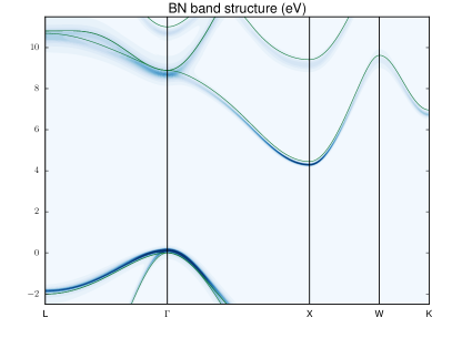
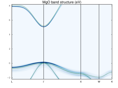
Figure 2: Spectral functions summed over the bands at each k-point of the Brillouin zone (arbitrary units). The green lines are the DFT band structure, in eV. When a quasiparticle peak is visible in the spectral function, the renormalization is infered from the difference of the position of that peak with the bare band structure. In the regions of flat bands, the band structure is being completely diffused. A satellite peak is seen below the last valence band of LiF and MgO.

II Anharmonic effects

Figure 3: Some of the high-order electron-phonon coupling diagrams which contribute to the self-energy. Each vertex with $n$ phonon branches is associated with a $n^{th}$-order derivative of the one-particle Hamiltonian. The independent-phonon approximation presented in the text retains only the diagrams formed with multiple interactions involving the same phonon mode.

The frozen-phonon method allows for a direct computation of the electron-phonon self-energy within the adiabatic approximation. We present here an extension of this method, which allows to explore anharmonic effects beyond the second-order perturbation theory of Allen, Heine and Cardona.

Recalling the theory of the harmonic crystal, we write the total energy in a frozen-phonon configuration as

$$E[\mathbf{z}]=E_{0}+\sum_{\nu}\frac{\omega_{\nu}^{2}}{2}z_{\nu}^{2},$$ (13)

where $E_{0}$ is the equilibrium fixed-ions energy, $z_{\nu}$ is a particular phonon coordinate and $\mathbf{z}$ denotes the ensemble of all of these coordinates. Taking the lattice dynamics into account, the phonon eigenstates are those of the decoupled harmonic oscillators:

$$\chi^{\mathbf{n}}(\mathbf{z})=\prod_{\nu}\chi^{n_{\nu}}(z_{\nu}),$$ (14)

where $\mathbf{n}$ denotes the ensemble of all the phonon occupation numbers. The total energy in this state is

$$E[\mathbf{n}]=E_{0}+\sum_{\nu}\omega_{\nu}\big{[}n_{\nu}+\tfrac{1}{2}\big{]}.$$ (15)

The expression for a particular eigenvalue at finite temperature is given by the derivative of $F=E-TS$, the Helmholtz free energy with respect to an electronic occupation number $f_{\lambda}$, which reduces to Poncé et al. (2014b)

$$\varepsilon_{\lambda}(T)=\frac{\partial F}{\partial f_{\lambda}}=\varepsilon_{\lambda}^{0}+\sum_{\nu}\frac{\partial\omega_{\nu}}{\partial f_{\lambda}}\big{[}n_{\nu}(T)+\tfrac{1}{2}\big{]}.$$ (16)

This expression should be compared with the electron-phonon self-energy in the adiabatic approximation (Eq. (5) and (12).) The individual phonon contributions to the self-energy are proportional to $\partial\omega_{\nu}/\partial f_{\lambda}$, which we call the electron-phonon coupling energies (EPCE). Using Brook’s theorem Poncé et al. (2014b), the EPCEs are given by the second-order derivatives of an eigenvalue with respect to a phonon coordinate:

$$\frac{\partial\omega_{\nu}}{\partial f_{\lambda}}=\frac{\partial\varepsilon_{\lambda}}{\partial n_{\nu}}=\frac{1}{2\omega_{\nu}}\frac{\partial^{2}}{\partial z_{\nu}^{2}}\ \varepsilon_{\lambda}\big{[}z_{\nu}\big{]}\Big{|}_{z_{\nu}=0},$$ (17)

where $\varepsilon_{\lambda}\big{[}z_{\nu}\big{]}$ is an electronic energy computed with all atoms displaced by a length $z_{\nu}$ along the phonon displacement vector $U^{\nu}_{\kappa j}$. This expression does not rely on the rigid-ion approximation, but requires a supercell calculation to account for the phonon wavevector. Within the validity of the rigid-ion approximation, it should reproduce the results of the static DFPT scheme. Both of these frameworks are developed within the harmonic approximation, since the total energy and the electronic eigenvalues are expanded up to second order in the phonon perturbations. Equivalently, the harmonic approximation can be defined as the assumption that the electronic eigenvalues vary quadratically with a phonon coordinate $z_{\nu}$.

In order to relax the harmonic approximation on the electronic energies, we cast the free energy $F=k_{B}T\ln Z$ in terms of the canonical partition function $Z=\text{Tr}\ e^{-\beta H}$, which is a trace over both the electronic and the atomic degrees of freedom. Resolving the trace over the electron coordinates, the expression for a temperature-dependent eigenvalue reads

$$\varepsilon_{\lambda}(T)=\int d\mathbf{z}\frac{e^{-\beta E[\mathbf{z}]}}{Z_{I}}\varepsilon_{\lambda}[\mathbf{z}],$$ (18)

where $Z_{I}=\int d\mathbf{z}\ e^{-\beta E[\mathbf{z}]}$ is the partition function of the atoms only, and $\varepsilon_{\lambda}[\mathbf{z}]$ is the eigenvalue computed in some frozen-phonon configuration. This formulation is reminiscent of the path-integral molecular dynamics approach Ramírez et al. (2006, 2008), with the difference that a configuration is specified in terms of phonon coordinates rather than atomic positions in real space. It retains the adiabatic approximation, since the atomic motion does not induce electronic transitions, but leaves the electrons in their evolving states.

We now use the crystal phonon structure and perform the harmonic approximation on the total energy only, writing

$$\varepsilon_{\lambda}(T)=\sum_{\mathbf{n}}\frac{e^{-\beta E[\mathbf{n}]}}{Z_{I}}\int d\mathbf{z}\big{|}\chi^{\mathbf{n}}(\mathbf{z})\big{|}^{2}\varepsilon_{\lambda}[\mathbf{z}].$$ (19)

We are assuming here that the set of phonon wavefunctions $\chi^{n_{\nu}}(z_{\nu})$ and frequencies $\omega_{\nu}$ computed from second-order perturbation theory are good eigenfunctions of the system. That is to say that the total energy is quadratic along the computed phonon modes even if the eigenvalues are not. Equation (19) now includes all high-order diagrams that may contribute to the self-energy, such as those depicted in Fig. 3.

Finally, we perform the independent phonon approximation and write

$$\varepsilon_{\lambda}(T)=\varepsilon_{\lambda}^{0}+\sum_{\nu}\sum_{n_{\nu}}s^{n_{\nu}}\int dz_{\nu}\big{|}\chi^{n_{\nu}}(z_{\nu})\big{|}^{2}\Big{(}\varepsilon_{\lambda}[z_{\nu}]-\varepsilon_{\lambda}^{0}\Big{)},$$ (20)

where $s^{n_{\nu}}=e^{-\beta\omega_{\nu}n_{\nu}}/\sum_{n_{\nu}^{\prime}}e^{-\beta\omega_{\nu}n_{\nu}^{\prime}}$. In doing so we disregard the cross-terms contributions between different phonons modes. This ansatz restricts the high-order diagrams to those containing a single phonon mode, which may interact multiple times with the electrons. These additional diagrams come from the anharmonicity of the eigenvalues appearing in the integrant of Eq. (20), as illustrated in Fig. 4. One can verify that if the eigenvalues vary quadratically with the phonon displacements, then Eq. (16) is recovered. Otherwise, Eq. (20) defines effective EPCEs for each phonon mode which include the anharmonic effects.

Results and discussion

We compute the EPCEs by frozen-phonon calculations, using the phonon displacement vectors obtained from DFPT. For the harmonic approximation, Eq. (17) is evaluated with atomic displacements of about $10^{-3}\AA$, while the anharmonic effects are included by evaluating Eq. (20) with $20$ displacements up to $\sim 0.3\AA$, which corresponds to about 4 units of a typical phonon average displacement $1/\sqrt{\omega_{\nu}}$.

The EPCEs are shown in Fig. 5 through the Brillouin zone of diamond. The spiky structure of the EPCEs of the first conduction band at $\Gamma$ results from this state not being at the bottom of the band. Consequently, when a phonon wavevector connects the state at $\Gamma$ to an other state with close energy, a divergence occurs in the EPCEs. A divergence also occurs for phonon wavevectors near $\Gamma$, for both the VB and CB states, but these divergences integrate to a finite value when the density of phonon modes is taken into account. The EPCEs computed with the frozen-phonon method in the harmonic approximation are in close agreement with the DFPT results, indicating that the rigid-ion approximation holds. However, when the full dependence of the eigenvalues on the phonon displacements is taken into account, the anharmonicity of the eigenvalues tend to reduce the EPCEs, with respect to the harmonic approximation.

This is exemplified on Fig. 4 with the mode $\Omega_{4}$ (the fourth mode with wavevectors $\Omega=(L+X)/2$). In the harmonic approximation, it contributes $-869$ meV to the CB EPCE at this q-point. The eigenvalue however departs from the quadratic behavior with the phonon displacement, reducing the coupling energy to $-383$ meV. On the other hand, the total energy follows closely the quadratic curve, indicating that this displacement is a genuine phonon mode. This tendency is observed near all divergent points of the Brillouin zone and near the zone center. The second-order perturbation theory is thus insufficient to treat the effect of those strongly coupling modes on the electronic states.

Table 3 reports the ZPR computed on a $4\times 4\times 4$ q-point grid with the various static schemes. Again, the total ZPR obtained with the harmonic frozen-phonon method and with DFPT are in good agreement. The discrepancies can be attributed to the rigid-ion approximation. When anharmonic effects are included, the total renormalization of the electronic energies is typically reduced compared to the harmonic approximation. For the indirect band gap materials, the renormalization of the CB state is largely affected by the anharmonic effects, since they receive an important contribution from those strongly coupling modes at the Brillouin zone boundaries which are being attenuated. The states at the band edges are being affected to various extends. The valence band of LiF, which is especially flat, shows a strong anharmonicity in the ZPR coming from the modes near $\Gamma$, reducing the ZPR by about $60\%$. In contrast, the conduction band of MgO, which is very dispersive, is only slightly affected by these effects.

Our results are obtained on a coarse q-point grid, limited by the scaling of the frozen-phonon method. Whether the same conclusions apply to a converged q-point grid depends on the relative importance of strongly coupling modes, since they are responsible for anharmonic effects. For the states lying at the top or at the bottom of their respective band, the ZPR increases monotonically with the number of q-points on a regular grid. This is because the region of strongly coupling phonon modes near $\Gamma$ gains in importance. Thus, the anharmonic effects for these state are expected to grow as a finer q-point sampling is achieved. For the states that are not at the extrema of their band, the convergence of the ZPR with q-points sampling is non-monotonic. In these cases, we cannot make quantitative predictions for the anharmonic effects on a converged q-point sampling. Nevertheless, the presence of strongly coupling modes near the Brillouin zone boundaries suggests an important anharmonic contribution to the ZPR.

Table 3: Zero-point renormalization of the band gap (in eV) within the adiabatic approximation, obtained whith the static DFPT, with the frozen-phonon method in the harmonic approximation (FPH), and with the frozen-phonon method including anharmonic effects (FPA).

		Static DFPT	FPH	FPA
C	VB	0.115	0.119	0.107
	CB	-0.320	-0.321	-0.214
	Gap	-0.436	-0.439	-0.320
BN	VB	0.120	0.133	0.108
	CB	-0.193	-0.198	-0.154
	Gap	-0.313	-0.331	-0.262
MgO	VB	0.110	0.118	0.070
	CB	-0.081	-0.078	-0.084
	Gap	-0.191	-0.196	-0.154
LiF	VB	0.445	0.431	0.168
	CB	-0.130	-0.122	-0.113
	Gap	-0.575	-0.553	-0.281

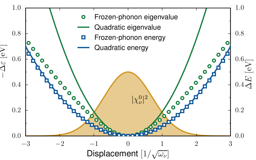
Figure 4: Dependence of the CB eigenvalue (green, circles) and the total energy (blue, squares) on a phonon displacement for the mode $\Omega_{4}$ of diamond. The circles and squares are the actual frozen-phonon calculations, the solid lines correspond to the harmonic approximation, and the filled curve is the phonon wavefunction.

Figure 5: Upper: The band structure of diamond, in eV. The dashed lines show the energies of the VB and CB states. Middle and lower: Electron-phonon coupling energies (EPCE), in eV for the CB state (middle) and the VB state (lower), computed with various methods. The blue line is the DFPT calculation, the yellow discs are the frozen-phonon method in the harmonic approximation, and the green triangles are the frozen-phonon method including anharmonic effects. A divergence is observed in the EPCEs of the CB state when a phonon wavevector couples this state to an other one with close energy, while the EPCE of both VB and CB states show a broad diverging peak at the center of the Brillouin zone.

III Conclusion

The dynamical DFPT scheme allowed us to compute the frequency-dependent electron-phonon coupling self-energy. Our calculations yield a renormalization factor ranging from $0.6$ to $1.0$. This renormalization factor is important to obtain correct quasiparticle energies, but has been laregly overlooked in the literature.

The spectral function reveals distinctive features of the quasiparticle band structure. In the indirect band gap materials (diamond and BN), the conduction bands undergo intra-band scattering processes, which broaden the spectral function at $\Gamma$. In the direct band gap materials with flat valence bands (LiF and MgO), these processes even generate satellite peaks below the valence bands.

The broadening can be obtained from the imaginary part of the self-energy, but one has to use a dynamical theory to do so. Not only are the phonon frequencies necessary to impose energy conservation in the scattering process, but the imaginary part of the self-energy must be evaluated at the renormalized eigenvalues, in order to compute properly the quasiparticle broadening.

Finally, we explored anharmonic effects using frozen-phonon calculations. The anharmonicity in the eigenvalue dependence on the atomic displacements occurs even if the phonon modes are correctly described by the second-order perturbation theory. This effect tend to decrease the contribution of the strongly coupling phonon modes, reducing the ZPR of certain states by as much as $60\%$ with respect to the static AHC theory.

Our results indicate that high-order electron-phonon coupling terms bring an important contribution to the self-energy and the ZPR. Our methodology however includes a partial summation of the high-order terms and treats the perturbations statically. A theory that would include all high-order terms in a dynamical way cannot be tested at present, but could be eventually addressed with quantum Monte-Carlo approaches.

Appendix A Imaginary parameter and convergence properties

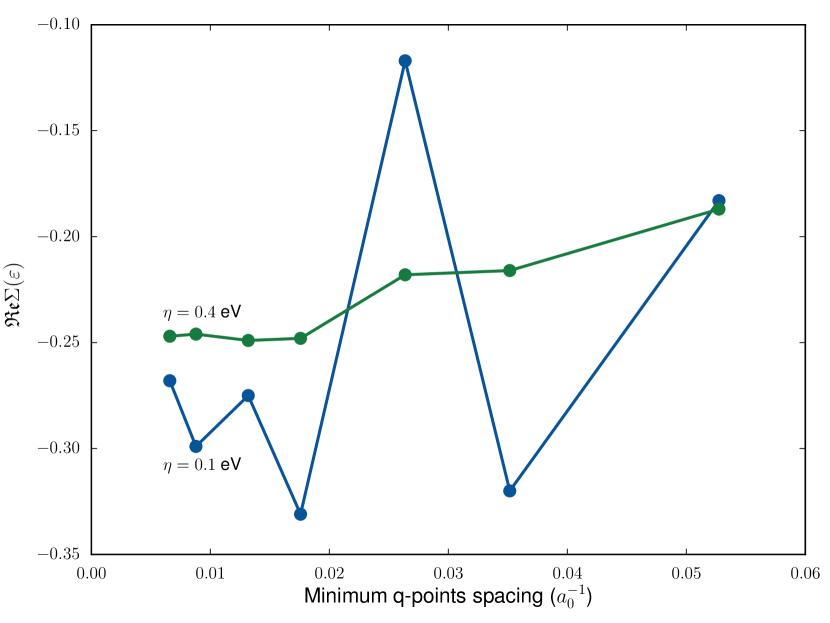
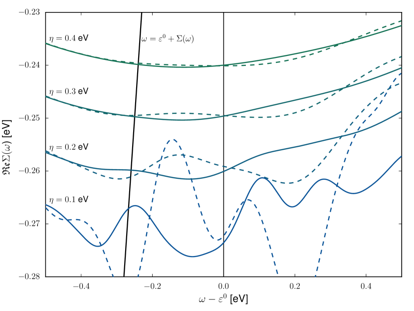
Figure 6: Upper: Convergence of the self-energy at the renormalized eigenvalue for the CB state of diamond, as a function of q-points spacing, with various imaginary parameters. Lower: Frequency dependence of the self-energy for the CB state of diamond, with various imaginary parameters. The solid lines are obtained on a $32\times 32\times 32$ q-point grid, and the dashed lines are obtained on a $24\times 24\times 24$ q-point grid, corresponding to the two left-most points on the upper pannel graph.

In order to compute the ZPR, one has to sample the phonon wavevectors in the Brillouin zone, either through a regular mesh, or with a random set of q-points. At the same time, one has to select a value for the parameter $\eta$ giving an imaginary part to the self-energy. The choice of this parameter should in facts be addressed in conjunction with the q-points sampling. When the static DFPT method is used, the numerical value assigned to $\eta$ is usually on the order of typical phonon frequencies ($\sim 0.1$ eV) to account for their omission. Otherwise, if a too small value of $\eta$ is used, it is not even clear that the self-energy will converge to a finite valuePoncé et al. (2015). In a dynamical scheme, one should in principle aim for a vanishing value for $\eta$. While it is expected that the self-energy elements should converge to a finite value as $\eta\rightarrow 0$, tuning the value of $\eta$ conveniently eases the convergence with the number of q-points, as shown in Fig. 6.

Moreover, using a too small value of $\eta$ can compromise the frequency dependence of the self-energy, as shown on Fig. 6 for the CB state of diamond. Even for the most converged q-point grid, the self-energy computed with $\eta=0.1$ eV shows rapid variations with $\omega$. These variations are even larger for a smaller q-point grid, and in these cases, the solution of $\omega=\Sigma(\omega+\varepsilon^{0})$ could certainly not be estimated by linearizing the self-energy near the bare eigenenergy. The self-energy becomes a perfectly smooth function of $\omega$ when $\eta=0.4$ eV.

We use the following criterion to determine the value of $\eta$. Consider the contribution of two neighboring q-points $\mathbf{q}$ and $\mathbf{q}^{\prime}$ to the self-energy of the electronic state $\mathbf{k}n$. The contribution of a particular electron band $n$ and phonon branch $m$ will have terms proportional to $\big{[}(\omega-\varepsilon^{0}_{\mathbf{k}+\mathbf{q}n}\pm\omega_{\mathbf{q}m}+i\eta)^{-1}+(\omega-\varepsilon^{0}_{\mathbf{k}+\mathbf{q}^{\prime}n}\pm\omega_{\mathbf{q}^{\prime}m}+i\eta)^{-1}\big{]}$, assuming that the matrix elements in the numerator of the self-energy does not change between $\mathbf{q}$ and $\mathbf{q}^{\prime}$. If the value of $\eta$ is vanishingly small, the spectral function will exhibit distinct peaks at $\omega=\varepsilon^{0}_{\mathbf{k}+\mathbf{q}n}\pm\omega_{\mathbf{q}m}$ and $\omega=\varepsilon^{0}_{\mathbf{k}+\mathbf{q}^{\prime}n}\pm\omega_{\mathbf{q}^{\prime}m}$, which will be an artifact of the q-points sampling. The separation of those peaks comes mainly from the dispersion of the electronic energies, which is more important than that of the phonon frequencies. Simple analysis shows that these peaks can be made undistinguishable by setting ${\eta=\sqrt{3}\Delta\varepsilon/2}$ where $\Delta\varepsilon=\varepsilon^{0}_{\mathbf{k}+\mathbf{q}n}-\varepsilon^{0}_{\mathbf{k}+\mathbf{q}^{\prime}n}$. Hence, for a given q-point mesh, we compute the largest $\Delta\varepsilon$ between neighboring q-points, within the bands being corrected, and use it to deduce $\eta$. The values of $\eta$ obtained for our most converged q-point grid are: $0.2$ eV for the VB state of diamond, $0.4$ eV for the CB states of diamond and BN, and $0.1$ eV for all the other VB and CB states. We verified that the broadening of the CB states of diamond and BN was insensitive to the choice of this parameter.

References

- Kioupakis et al. (2010) E. Kioupakis, P. Rinke, A. Schleife, F. Bechstedt, and C. G. Van de Walle, Physical Review B 81, 241201 (2010).
- Noffsinger et al. (2012) J. Noffsinger, E. Kioupakis, C. G. Van de Walle, S. G. Louie, and M. L. Cohen, Physical Review Letters 108, 167402 (2012).
- Wang et al. (2011) Z. Wang, S. Wang, S. Obukhov, N. Vast, J. Sjakste, V. Tyuterev, and N. Mingo, Physical Review B 83, 205208 (2011).
- Cardona (2006) M. Cardona, Science and Technology of Advanced Materials 7, S60 (2006).
- Giustino et al. (2007) F. Giustino, J. R. Yates, I. Souza, M. L. Cohen, and S. G. Louie, Physical Review Letters 98, 047005 (2007).
- Lee and Pickett (2004) K.-W. Lee and W. E. Pickett, Physical Review Letters 93, 237003 (2004).
- Blase et al. (2004) X. Blase, C. Adessi, and D. Connétable, Physical Review Letters 93, 237004 (2004).
- Cardona and Thewalt (2005) M. Cardona and M. L. W. Thewalt, Reviews of Modern Physics 77, 1173 (2005).
- Restrepo et al. (2009) O. D. Restrepo, K. Varga, and S. T. Pantelides, Applied Physics Letters 94, 212103 (2009).
- Tyuterev et al. (2011) V. G. Tyuterev, S. V. Obukhov, N. Vast, and J. Sjakste, Physical Review B 84, 035201 (2011).
- Bhattacharya et al. (2015) R. Bhattacharya, R. Mondal, P. Khatua, A. Rudra, E. Kapon, S. Malzer, G. Döhler, B. Pal, and B. Bansal, Physical Review Letters 114, 047402 (2015).
- King-Smith et al. (1989) R. D. King-Smith, R. J. Needs, V. Heine, and M. J. Hodgson, EPL (Europhysics Letters) 10, 569 (1989).
- Capaz et al. (2005) R. B. Capaz, C. D. Spataru, P. Tangney, M. L. Cohen, and S. G. Louie, Physical Review Letters 94, 036801 (2005).
- Allen and Heine (1976) P. B. Allen and V. Heine, Journal of Physics C: Solid State Physics 9, 2305 (1976).
- Allen and Cardona (1981) P. B. Allen and M. Cardona, Physical Review B 23, 1495 (1981).
- Allen and Cardona (1983) P. B. Allen and M. Cardona, Physical Review B 27, 4760 (1983).
- Zollner et al. (1991) S. Zollner, S. Gopalan, and M. Cardona, Solid State Communications 77, 485 (1991).
- Zollner et al. (1992) S. Zollner, M. Cardona, and S. Gopalan, Physical Review B 45, 3376 (1992).
- Garro et al. (1996) N. Garro, A. Cantarero, M. Cardona, A. Göbel, T. Ruf, and K. Eberl, Physical Review B 54, 4732 (1996).
- Olguin et al. (2002) D. Olguin, M. Cardona, and A. Cantarero, Solid State Communications 122, 575 (2002).
- Baroni et al. (1987) S. Baroni, P. Giannozzi, and A. Testa, Physical Review Letters 58, 1861 (1987).
- Baroni et al. (2001) S. Baroni, S. de Gironcoli, A. Dal Corso, and P. Giannozzi, Reviews of Modern Physics 73, 515 (2001).
- Gonze (1997) X. Gonze, Physical Review B 55, 10337 (1997).
- Gonze and Lee (1997) X. Gonze and C. Lee, Physical Review B 55, 10355 (1997).
- Marini (2008) A. Marini, Physical Review Letters 101, 106405 (2008).
- Note (1) See for example some of the largely cited article introducing DFPT Baroni et al. (1987); Gonze (1997).
- Laflamme Janssen et al. (2010) J. Laflamme Janssen, M. Côté, S. G. Louie, and M. L. Cohen, Physical Review B 81, 073106 (2010).
- Faber et al. (2011) C. Faber, J. L. Janssen, M. Côté, E. Runge, and X. Blase, Physical Review B 84, 155104 (2011).
- Lazzeri et al. (2008) M. Lazzeri, C. Attaccalite, L. Wirtz, and F. Mauri, Physical Review B 78, 081406 (2008).
- Yin et al. (2013) Z. P. Yin, A. Kutepov, and G. Kotliar, Physical Review X 3, 021011 (2013).
- Antonius et al. (2014) G. Antonius, S. Poncé, P. Boulanger, M. Côté, and X. Gonze, Physical Review Letters 112, 215501 (2014).
- Poncé et al. (2014a) S. Poncé, G. Antonius, P. Boulanger, E. Cannuccia, A. Marini, M. Côté, and X. Gonze, Computational Materials Science 83, 341 (2014a).
- Gonze et al. (2011) X. Gonze, P. Boulanger, and M. Côté, Annalen der Physik 523, 168 (2011).
- Giustino et al. (2010) F. Giustino, S. G. Louie, and M. L. Cohen, Physical Review Letters 105, 265501 (2010).
- Cannuccia and Marini (2011) E. Cannuccia and A. Marini, Physical Review Letters 107, 255501 (2011).
- Cannuccia and Marini (2012) E. Cannuccia and A. Marini, The European Physical Journal B 85, 320 (2012).
- Rignanese et al. (1996) G.-M. Rignanese, J.-P. Michenaud, and X. Gonze, Physical Review B 53, 4488 (1996).
- Monserrat et al. (2013) B. Monserrat, N. D. Drummond, and R. J. Needs, Physical Review B 87, 144302 (2013).
- Paulatto et al. (2013) L. Paulatto, F. Mauri, and M. Lazzeri, Physical Review B 87, 214303 (2013).
- Gonze et al. (2009) X. Gonze, B. Amadon, P.-M. Anglade, J.-M. Beuken, F. Bottin, P. Boulanger, F. Bruneval, D. Caliste, R. Caracas, M. Côté, T. Deutsch, L. Genovese, P. Ghosez, M. Giantomassi, S. Goedecker, D. Hamann, P. Hermet, F. Jollet, G. Jomard, S. Leroux, M. Mancini, S. Mazevet, M. Oliveira, G. Onida, Y. Pouillon, T. Rangel, G.-M. Rignanese, D. Sangalli, R. Shaltaf, M. Torrent, M. Verstraete, G. Zerah, and J. Zwanziger, Computer Physics Communications 180, 2582 (2009).
- Marini et al. (2015) A. Marini, S. Poncé, and X. Gonze, Physical Review B 91, 224310 (2015).
- Mahan (2000) G. D. Mahan, Many-Particle Physics, third edition ed. (Kluwer Academic / Plenum Publishers, New York, 2000).
- Poncé et al. (2014b) S. Poncé, G. Antonius, Y. Gillet, P. Boulanger, J. Laflamme Janssen, A. Marini, M. Côté, and X. Gonze, Physical Review B 90, 214304 (2014b).
- Tjeng et al. (1990) L. H. Tjeng, A. R. Vos, and G. A. Sawatzky, Surface Science 235, 269 (1990).
- Ramírez et al. (2006) R. Ramírez, C. P. Herrero, and E. R. Hernández, Physical Review B 73, 245202 (2006).
- Ramírez et al. (2008) R. Ramírez, C. P. Herrero, E. R. Hernández, and M. Cardona, Physical Review B 77, 045210 (2008).
- Poncé et al. (2015) S. Poncé, Y. Gillet, J. L. Janssen, A. Marini, M. Verstraete, and X. Gonze, The Journal of Chemical Physics 143, 102813 (2015).