Bayesian Trend Filtering
Abstract
We develop a fully Bayesian hierarchical model for trend filtering, itself a new development in nonparametric, univariate regression. The framework more broadly applies to the generalized lasso, but focus is on Bayesian trend filtering. We compare two shrinkage priors, double exponential and generalized double Pareto. A simulation study, comparing Bayesian trend filtering to the original formulation and a number of other popular methods shows our method to improve estimation error while maintaining if not improving coverage probability. Two time series data sets demonstrate Bayesian trend filtering’s robustness to possible violations of its assumptions.
Keywords: Bayesian analysis, trend filtering, locally adaptive regression splines, nonparametric
1 Introduction
Consider the nonparametric model of the function , with zero mean, independent, Gaussian errors
| (1) |
Assume the observations are generated via from the unique inputs . Mammen and van de Geer (1997) propose an estimator of , convergent at the minimax rate, by penalizing the total variation of the derivative of the function , taken to be
with the set of knots equal to the inputs. Since the penalty TV is not easily computed, an alternative solution uses an estimate of the total variation penalty. Consider the estimator of that solves
where is taken to be the vector of responses. R. J. Tibshirani (2014) proposed such an estimator that maintains the optimal (minimax) convergence rate. His method, called trend filtering, estimates TV using the divided difference of order of . DeVore and Lorentz (1993) and de Boor (2005) provide two excellent references on the divided difference.
Trend filtering uses the generalized lasso framework (Tibshirani, 2014). Assume and a model matrix . The generalized lasso finds the minimum vector constrained by a linear transformation
| (2) |
for some penalty parameter . Trend filtering uses the minimization problem in Equation (2) with and by cleverly choosing a penalty matrix that when coupled with the norm recovers an estimate of the total variation penalty.
We adapt trend filtering, as a special case of the generalized lasso, to the Bayesian setting. Similar efforts to fit lasso type, or other general shrinkage, problems with a hierarchical Bayesian model have been made (see Park and Casella, 2008; Hans, 2009; Kyung et al., 2010; Griffin and Brown, 2011; Lee et al., 2012). We further investigate Bayesian trend filtering with another shrinkage prior, the generalized double Pareto, as developed by Lee et al. (2010) and Armagan et al. (2013). The generalized double Pareto prior, when applied to Bayesian trend filtering, appears to estimate the true, underlying function with smaller error and to provide better frequentist coverage properties than does the more standard double exponential prior.
This paper reads as follows. Section 2 discusses trend filtering, its minimax convergence rate and standard errors. We present Bayesian trend filtering and details on its implementation in Section 3. A simulation study comparing original trend filtering to the Bayesian version, and both of these to some popular univariate, nonparametric regression methods, is carried out in Section 4.1. Section 4.2 fits these methods to two real data sets. Section 5 briefly mentions Bayesian trend filtering’s relation to Gaussian process regression, summarizes our findings, and mentions some future research directions.
2 Trend Filtering
Trend filtering, as discussed here, was developed in two stages. Kim et al. (2009) first introduced trend filtering for piecewise linear fits, providing a primal-dual interior point algorithm to fit the method at a specified value of the penalty parameter, . Tibshirani (2011) next identified trend filtering as a special case of the generalized lasso, thus offering a path algorithm that fits trend filtering over all values of the penalty parameter, . In a separate paper Tibshirani (2014) established convergence properties of the method. In the end, trend filtering fits a piecewise polynomial of order with knots taken to be the set of inputs . The piecewise polynomial comes from a continuous-time representation of the following discrete minimization problem,
| (3) |
The discrete difference matrix depends both on the order of the derivative of the function , as chosen by the practitioner, and the inputs . The penalty term estimates the total variation of the th derivative of the function . Because of this close relation to locally adaptive regression splines, trend filtering adapts to the fluctuations of the underlying curve and thus achieves the same optimal convergence rate (Tibshirani, 2014).
2.1 Minimax Convergence Rate
Trend filtering converges at the minimax rate to the true underlying function of interest, as is shown by Tibshirani (2014). He used purely algebraic methods to show that trend filtering is sufficiently close to the locally adaptive regression spline estimator for the minimax convergence rate to carry over to trend filtering. It is well known that this convergence rate is not achieved by any estimator linear in (Donoho and Johnstone, 1998; Tibshirani, 2014). Thus, the optimal convergence rate depends on the norm.
Another strategy to prove the minimax convergence rate for trend filtering would make use of the metric entropy of the underlying function space for which trend filtering finds its solution. This strategy is analogous to that of Mammen and van de Geer (1997) for locally adaptive regression splines. Tibshirani (2014) briefly mentions the difficulty of such a proof. The requisite interpolating properties of trend filtering are quite difficult to establish because trend filtering uses piecewise polynomials with potentially discontinuous lower order derivatives. We mention this alternative strategy, not because we were able to over-come the aforementioned difficulties, but instead to highlight how Bayesian trend filtering could share metric entropy proofs of convergence rates across penalized regression and Gaussian process regression methods. This connection is discussed further in Section 5.
2.2 Standard Errors
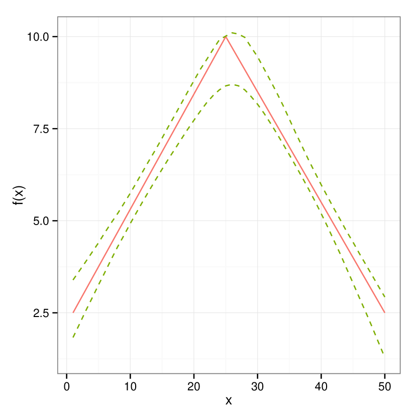
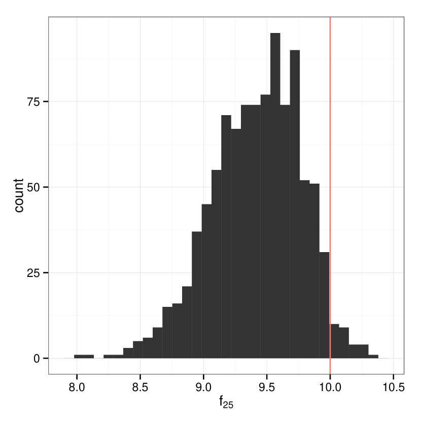
As is summarized in Kyung et al. (2010), estimating the standard errors of lasso problems is quite difficult. This is also seen by the significant amount of attention paid to the problem; for example, see (Tibshirani, 1996; Knight and Fu, 2000; Osborne et al., 2000; Fan and Li, 2001; Pötscher and Leeb, 2009). However, with trend filtering the theory cited here does not find easy evidence. Figure 1 displays % and % quantiles of bootstrapped function evaluations at each input, for a simple piecewise linear function (solid red). The % confidence intervals (green dash) provide seemingly reasonable estimates of error. The only obvious problem seen in Figure 1 is the bias indicated by the histogram of the bootstrapped estimates of .
Cross validation, the recommended method to estimate , is both computationally costly and is well known to encourage over-fitting (Davison, 1997). If you are willing to trade speed for an inexact solution, it is reasonably easy to overcome the computational cost of bootstrapping after one estimates the penalty parameter. For instance, we could estimate a trend filtering fit using the majorization-minimization techniques of Hunter and Li (2005). An approximation to objective function (3), details of which are provided in Appendix A, quickly allows us to refit trend filtering given a new set of observations and a pre-calculated penalty parameter, say , estimated from -fold cross validation. Though this strategy is itself limited, it is quite fast. For a fixed value of , it took a MacBook Pro GHz Intel Core i just about half the time to calculate bootstrapped approximations of in Figure 1, with , as it did to fit the exact solution of trend filtering and estimate . In general, we found this approximation strategy to produce estimates relatively close to the exact fit. It was common to see mean absolute differences on the order of . However, cross validation for trend filtering frequently produces estimates of the true function that are too “wiggly.” Bootstrap methods that then rely on will also produce poor results. The simulations and especially the real data sets presented in Section 4.1 highlight this point exactly. When the estimates of under are too wiggly, bootstrapped confidence intervals fail to contain the true function across the sampled domain, thus lowering nominal coverage probability.
The problem with choosing , in our experience, largely disappears under the Bayesian approach. Bayesian trend filtering estimates by incorporating it into the hierarchical model (4) so that the estimates of are marginalized over all values of . This encourages a more robust, stable estimate of . The results in Section 4.1 justify our conclusions about both trend filtering and Bayesian trend filtering.
3 Bayesian Trend Filtering
3.1 Formulation
Similar to the work of Park and Casella (2008); Kyung et al. (2010); Griffin and Brown (2011), and Armagan et al. (2013), a fully Bayesian hierarchical model for Bayesian trend filtering can be expressed as a scale mixture of normals, a mixture that was first discovered by Andrews and Mallows (1974). The resulting hierarchical model puts a double exponential (dexp)
conditional prior on the penalty term . Park and Casella (2008) show that the double exponential prior conditional on ensures that the joint posterior distribution of is unimodal. The fully Bayesian hierarchical model to fit Bayesian trend filtering is
| (4) | ||||
The are mutually independent, and throughout we let , which is the limiting improper prior from an inverted gamma distribtion. The distribution on , denoted by , highlights the fact that a slight change of the prior will produce two different conditional prior distributions. The more common, double exponential conditional prior is found by letting be a gamma distribution on (Park and Casella, 2008; Kyung et al., 2010). Additionally, we consider a variation on the prior developed by Lee et al. (2010, 2012), and Armagan et al. (2013) which uses a prior on instead of . The generalized double Pareto (gdp) distribution takes on the following form within Bayesian trend filtering,
The gdp is known to eschew much of the bias otherwise induced by the exponential tails of the double exponential distribution (Lee et al., 2010). We explore the choice of hyperparameters in Section 4.1.
A simplie Gibbs sampler provides samples from the posterior distributions of interest for Bayesian trend filtering. The full conditionals shared by both conditional priors are
The full conditional of for dexp is , and relative to gdP, .
Model (4) can be viewed as an extension of the work in Kyung et al. (2010). Therefore, we appeal to their Propositions and which show that the underlying Gibbs sampler is geometrically ergodic. The two Gibbs samplers, for dexp and gdp, converge both in theory and in practice very quickly.
Proposition 3.1.
The Gibbs sampler for the hierarhcical model (4) is geometrically ergodic.
We refer the reader to the proof by Kyung et al. (2010). In Section 5, we show that Proposition 3.1 can help reduce the computational cost of Bayesian trend filtering.
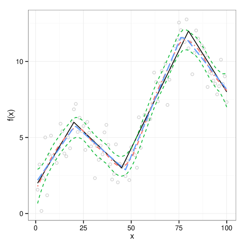
A few points contrasting trend filtering with Bayesian trend filtering should be noted. Trend filtering, by restricting the parameter space of the objective function (3), automatically sets some terms in the penalty to exactly zero. Such a data dependent selection of important predictors is philosophically appealing. Within trend filtering, this data dependent selection corresponds to setting esimates of the terms in the total variation of to zero. Bayesian trend filtering, however, never sets any terms identically to zero. Figure 2 compares Bayesian trend filtering to the original trend filtering formulation. Bayesian trend filtering doesn’t quite predict a piecewise linear function when in fact the true function is a piecewise linear function, with three knots at equal to , and . What Bayesian trend filtering sacrifices in knot detection, it makes up for when fitting smooth curves. The information gained by incorporating into the Gibbs sampler, and the propagation of that information back to the estimates of provides stable estimation, as is shown in Section 4. Thus, the primary advantage of Bayesian trend filtering is as a smoother and not as a knot-detection method.
3.2 Computational Considerations
The very idea of the (generalized) lasso, to shrink some of the elements of the penalty term towards zero possibly setting some to exactly zero, can cause computational issues in the Bayesian setting. Consider the full conditional , for either conditional prior dexp or gdp. The mean in the inverse-Gaussian distribution inverts exactly that which we are shrinking towards zero. Any sample from the posterior distribution such that an element of the penalty term is very close to zero, threatens numerical stability when drawing samples from the already rather numerically sensitive inverse-Gaussian distribution; see (Wheeler, 2013) and the references there within. With Bayesian trend filtering, when an element of is too small, simulating a draw from can return a value less than or equal to zero – obviously a problem for a distribution with non-negative support. To ameliorate such issues, we propose the admitedly inelegant solution of resampling the entire vector if any element of is less than . We find that resampling happens less than five percent of time. Further, when resampling does occur, it is extremely rare that more than one resample is ever needed. Despite such numerical issues, restricting the support of specific posterior distributions does not appear to hinder Bayesian trend filtering’s performance; see Section 4.1.
4 Numerical Results
4.1 Simulations
We compare Bayesian trend filtering (BTF), with both conditional priors dexp and gdp, against three different methods: trend filtering (TF) from Tibshirani (2014), Bayesian additive regression trees (BTree) from Chipman et al. (2010); Kapelner and Bleich (2013), and cubic smoothing splines CSM from Wood (2006). BTree is included as it is becoming an increasingly popular Bayesian regression method. We include smoothing splines as they are arguably the most used method of smoothing, and also to highlight a different point than was made of the same comparison by Tibshirani (2014). There, a strong argument was made for the efficiency of TF, implicitly defined to be mean squared error (mse) per degree of freedom. In that world, TF clearly stands above as its asymptotic results are shown to benefit finite sample sizes. Here, a more applied world is hypothesized, where estimation of further dictates a methods performance.
A functions used in the simulations are from various R (Core Team, 2014) packages. BTree was fit with bartMachine::bartMachine using the default values of trees and (after burn-in) iterations (Kapelner and Bleich, 2013). CSM was fit using the cubic smoothing spline function mgcv::gam, with all inputs used as knots (to make more fair the comparison between CSM and the trend filtering methods). TF was fit with genlasso::trendfilter using a cubic piecewise polynomial, with both - and -fold cross validation (Tibshirani, 2014). BTF, also using a cubic piecewise polynomial, was fit using btf:btf with (after burn-in) posterior samples (Roualdes, 2014). Since the choice of hyperparameters and effects the overall fit of both BTF-gdp and BTF-dexp, we explore Bayesian trend filtering’s responsiveness to changes in these hyperparameters. We fit BTF-dexp with and , and BTF-gdp with each of and . We chose a number of “small” values of to ensure a true thresholding rule, and thus encourage shrinkage (Armagan et al., 2013).
For simulated data, we consider two univariate functions with regularly spaced inputs. The first, a piecewise cubic function is borrowed from Tibshirani (2014). The second is a difficult, spatially inhomogeneous function, colloquially known as dampened harmonic motion (dhm). replications of these two functions with three different levels of normal noise are evaluated upon three criteria. For each replication we calculate the mean and standard deviation of the mean squared errors (mse) and confidence intervals for both the underlying function evaluated at all inputs and the variance. bootstrap samples were used to estimate confidence intervals of function estimates for TF, while CSM used the method predict.gam to obtain standard errors. All frequentist methods relied on the bootstrap to estimate . We used posterior samples to create credible intervals for all the Bayesian methods. Thus, the replications are used to estimate the mean and standard deviation of the mses, and overall mean and standard errors of the two different coverage probabilities.
The real world data consists of two data sets common to the smoothing literature. The first is a dataset of global mean surface temperature deviations for the years to from Hodges (2013). The second is the SILSO dataset, monthly sunspot counts for the years .
4.1.1 Piecewise Cubic
Of the three levels of noise, , for the piecewise cubic function with , the right plot of Figure 3 shows the mses of replications of observations from the true function (solid black) displayed in the left plot. The BTF methods displayed in this plot used the hyperparameter values of and . These plots are representative of all cases of the BTF methods for which , inclusive of all the tested values of . BTF clearly produces mses with lower variance, although most methods save BTree (not shown) provide practically the same median mse. Still, BTF-gdp in Figure 3 provided nearly the smallest set of mses: there are and fits from TF and CSM, respectively, where the mse is greater than the largest mse for BTF-gdp. And conversely, there are no fits that provide an mse smaller than the smallest mse from BTF-gdp. Table 1 provides mean and standard deviations of the mses for the different methods across all levels of noise chosen for the piecewise cubic function.
The left plot of Figure 3 displays the fits with the greatest mse of BTF-gdp and CSM. The BTF methods appear to minimize the worst of the fits to the piecewise cubic function. We highlight BTF-gdp because it almost unanimously outperforms BTF-dexp in all of our examples and we highlight CSM because it is the next best method, outside of the BTF methods, in terms of methods with extreme mse values.
| method | mean | sd | mean | sd | mean | sd |
|---|---|---|---|---|---|---|
| BTF-dexp | ||||||
| BTF-gdp | ||||||
| TF | ||||||
| CSM | ||||||
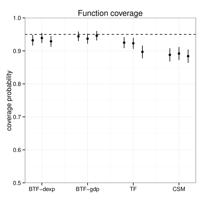
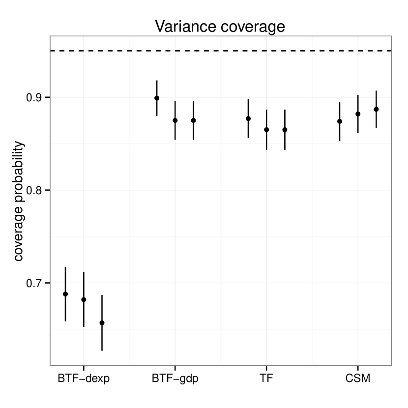
Consistent function estimation by BTF is seen when we compare coverage probabilities. Figure 4 plots the mean plus/minus two standard errors, at every level of noise, of function and variance coverage probabilities. Since we measured function coverage across the entire domain, the over-fitting of CSM and TF reduced their respective function coverage probabilities. Moreover, no method appropriately covered the variance at the nominal value. We notice, though do not provide plots of such here, that both BTF methods’ variance coverage declines as the hyperparameter increases.
While BTree (not shown) provides reasonably small mses for the piecewise cubic function, it had the highest median mse. This is largely due to the fact that it is not a smoothing technique. BTree was removed from the plots throughout as it distracted from the main comparisons of interest. Still, BTree did quite well estimating the variance. In other contexts, where a smooth fit is not necessary, BTree has much to offer beyond what most of these smoothing techniques are able to handle.
4.1.2 Spatially Inhomogeneous
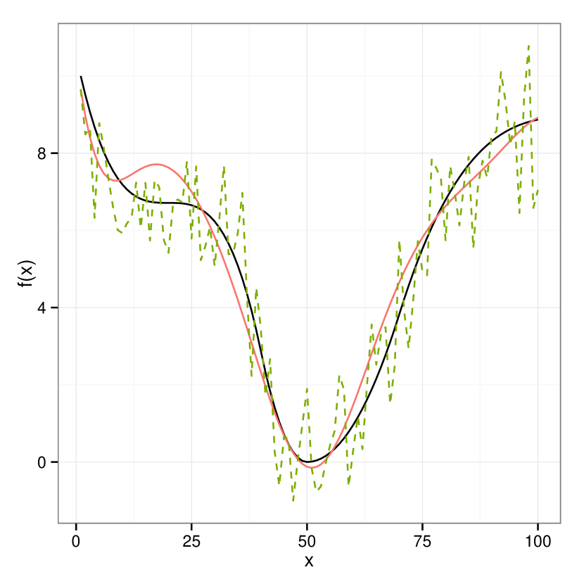
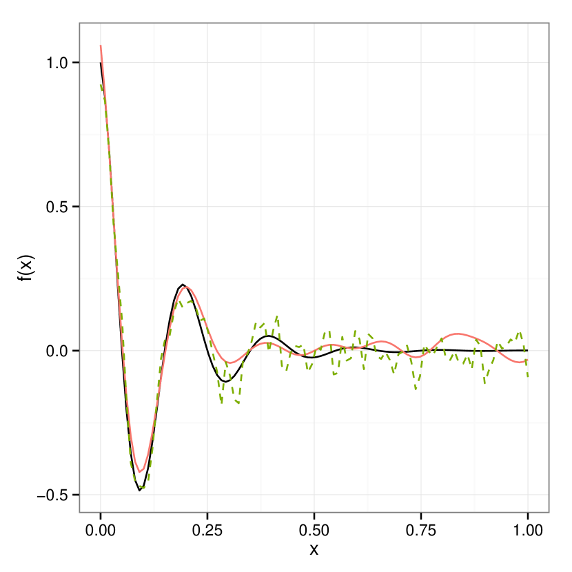
The second example uses the spatially inhomogeneous function
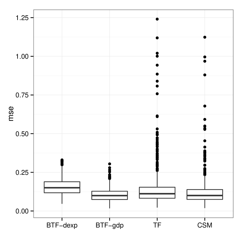
with noise and . Figure 5 again plots the true function (solid black) on the left and all mses on the right, for the noise level . The BTF methods presented for dampened harmonic motion use the same hyperparameter values as for the piecewise cubic function, and . Like with the piecewise cubic function, these hyperparameter values generally represent the all hyperparameter choices where . In Figure 5 we see that all trend filtering methods produce nearly identical median mses. The over-fitting is still a problem for CSM and TF. Also, notice that the median mse for the cubic smoothing spline method CSM is a bit larger than the median mses for the trend filtering methods. Table 2 summarizes the mses for all levels of noise for the dampened harmonic motion function. The BTF methods provide the smallest mean mses, with the smallest standard deviation, for all levels of noise considered.
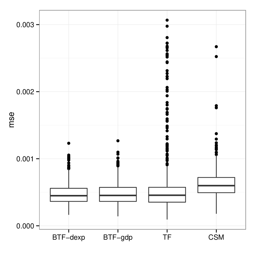
Generally with the dampened harmonic motion, as judged by mses, the BTF methods again perform well. In this case, BTF-dexp performs insignificantly better than BTF-gdp. This could be due to the heavy smoothing, required for dapmened harmonic motion, that the exponential tails of dexp encourage. Still, BTF-gdp gives smaller mean mses with smaller variation than the other methods. Greater than the largest mse of BTF-gdp there exists and mses as produced by TF and CSM, respectively. Only TF provides any, specifically two, simulations with a smaller mse than that of BTF-gdp.
| method | mean | sd | mean | sd | mean | sd |
|---|---|---|---|---|---|---|
| BTF-dexp | ||||||
| BTF-gdp | ||||||
| TF | ||||||
| CSM | ||||||
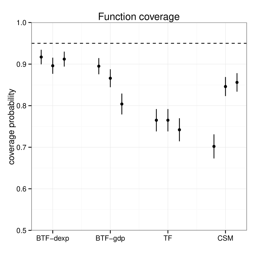
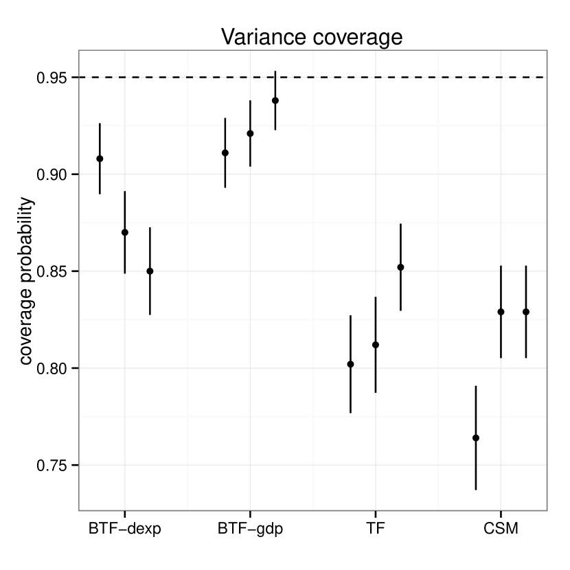
Figure 6 shows function and variance coverage probability means plus/minus two standard errors for the all levels of noise of the dampened harmonic motion function. Function estimation proved difficult for all the methods. This is likely do to the fact that we are measuring overall function coverage on a quite spatially inhomogeneous function. Still for many values of the hyperparameters, the BTF methods perform well in terms of function coverage probability, as is seen in the left plot of Figure 6. As for variance coverage, BTF-dexp does noticeably worse than BTF-gdp, which itself outperforms the other methods.
4.2 Real Data Analysis
4.2.1 Surface Temperatures
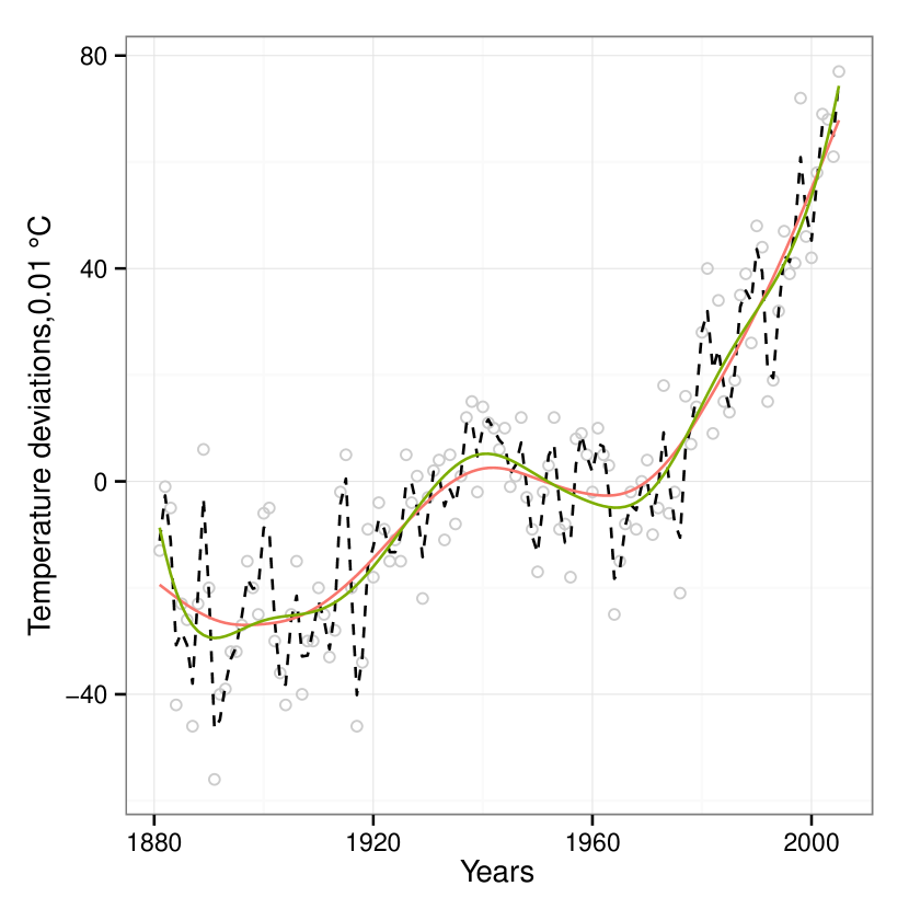
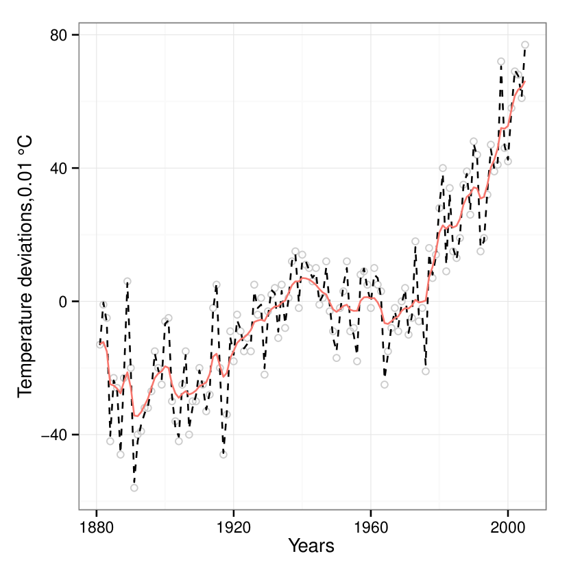
The global surface temperature deviations data consist of yearly, , measurements in units of . Figure 7 displays various fits to these data. The global surface temperature data proves to be a problem for both -fold cross validation used by TF (dash black), as is seen in the right plot of Figure 7. Trend filtering essentially fits every data point. BTF-gdp (solid green), where and , smooth these data toward the hypothesized underlying function as seen in the left plot of Figure 7. Because the trend filtering methods assume independent observations, possibly an incorrect error strucutre for these data, we also fit CSM with an autoregressive one, denoted AR(1), error structure (solid red). We find that the estimates of BTF-gdp and CSM with an AR(1) error structure, displayed in the left plot of Figure 7, are quite similar. In fact, BTF-gdp’s credible intervals (not shown) completely contain the CSM autoregressive one fit.
4.2.2 Sunspots
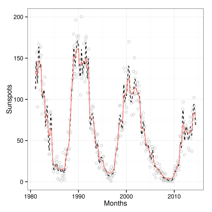
The second applied data set we investigate is monthly sunspot counts over the years to , with observations (Center, 1980-2014). In the left plot of Figure 8, BTF-gdp (solid green) with and provides a nice smooth fit to these data. In the right plot of Figure 8, we see that TF (dash black) using -fold cross validation provides a noisy fit to these data. Both - and -fold cross validation provide nearly the same fit to these data. BTree (solid red), in the left plot, provides a slightly less noisy estimate of these data than did TF.
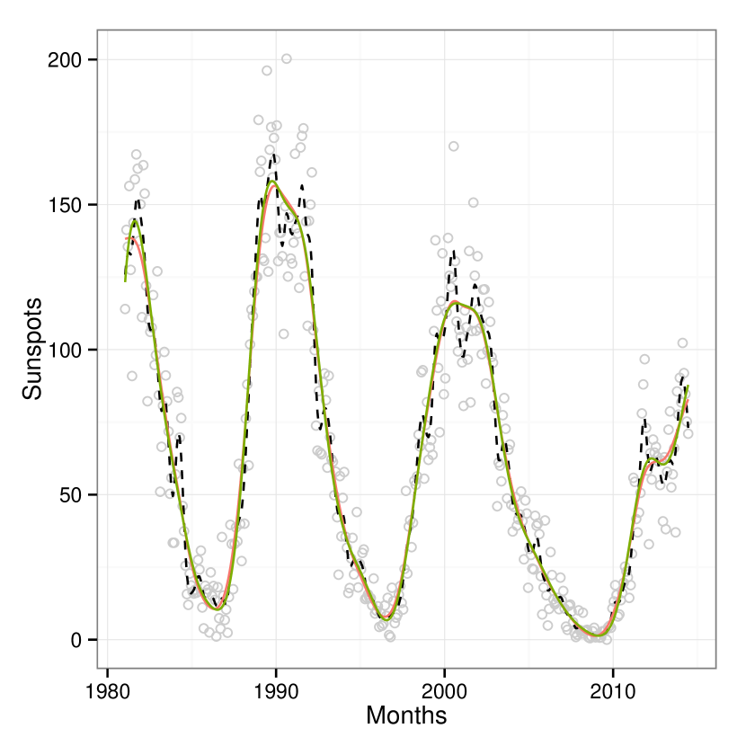
Similar concerns about a possibly misspecified error structure exist for these data when applying the trend filtering methods. We therefore fit CSM with an AR(1) error structure (solid red), as seen in the left plot of Figure 8. As with the temperature data, the BTF-gdp (solid green) and CSM-AR(1) fits are quite similar, again the estiamtes of CSM-AR(1) are completely contained by the credible intervals (not shown) of BTF-gdp. It is unclear which assumption is more appropriate for the underlying physical process of these data: correlated errors as in CSM with an AR(1) error structure, or a function with evaluations correlated across time and uncorrelated errors, as Bayesian trend filtering assumes.
5 Discussion
We developed a Bayesian, nonparametric smoother that finds its origins in the lasso literture. Our method uses a simple scale mixture of normals to build a fully Bayesian hierarchical model. The hierarchical model of Bayesian trend filtering closely resembles the structure of Gaussian process regression, albeit with a unique covariance function that is best understood in terms of the underlying penalty; see Rasmussen (2006) for a thorough review of Gaussian processes. Bayesian trend filtering, in this way, lives in the intersection of penalized regression, namely the (generalized) lasso, and the Gaussian process prior literature. From this vantage point, we found two distinct bodies of research that offer the framework for a proof of the convergence rate of Bayesian trend filtering.
Bayesian trend filtering is closely related to the work of Mammen and van de Geer (1997) on locally adaptive regression splines. To show that locally adaptive regression splines are convergent at the minimax rate, Mammen and van de Geer (1997) use the metric entropy calculations of Van de Geer (1990); Mammen (1991) and also interpolating properties of splines developed by de Boor (2001). Building on this work, Tibshirani (2014) proves a similar conclusion for trend filtering. On the other hand, Bayesian trend filtering uses a hierarchical model common to Gaussian process regression. Some in the Gaussian process literature have a similar goal in mind: prove rates of convergence of posterior distributions that are based on Gaussian process priors (Ghosal et al., 2007; Van der Vaart and Van Zanten, 2008; Van Der Vaart and Van Zanten, 2011). This work on Gaussian process priors, which contains Bayesian trend filtering, notes that at the heart of the metric entropy proofs relating to nonparametric regression, there lies interpolating properties of the function space of interest (Ghosal et al., 2007). Though we were not able to prove such interpolation properties about the space of piecewise polynomials, this connection between penalized regression techniques and the Gaussian process regression methods is quite interesting.
Bayesian trend filtering has good potential in application. Based on our simulations, we find that Bayesian trend filtering has good estimation and strong frequentist properties, as compared to the original trend filtering and a popular cubic smoothing spline method. These benefits come from both the penalty, which acts similar to the total variation penalty, and the ability to estimate well the penalty parameter . We also found that the generalized double Pareto conditional prior provides a substantial increase in Bayesian trend filtering’s accuracy and coverage probablities. Overall, Bayesian trend filtering decreases estimation error compared to the other methods we tested.
Bayesian trend filtering’s benefits though come at some cost. Bayesian trend filtering relies on a matrix inversion within the full conditional at every iteration. This matrix inverse is the most significant computational cost of Bayesian trend filtering, and it puts the method’s computational complexity to be . Though, it should be reemphasized that depsite the computational burden, more information is gained from a Bayesian trend filtering fit. Some in the Gaussian process literature developed means to avoid such an inverse in special cases, for instance see Vehtari and Vanhatalo (2007); Liu et al. (2014), but these methods are not directly applicable to Bayesian trend filtering.
A simplistic strategy to reduce the computation time for Bayesian trend filtering uses the Gibbs sampler’s fast convergence rate. From Proposition 3.1 and from our simulations, we know that the Gibbs sampler of Bayesian trend filtering converges very quickly. We could reduce computational complexity by sampling from the full conditional for every th iteration, while sampling all other full conditionals every iteration. This would reduce the computational burden of the full conditional , but at the same time produce larger effective sample sizes for the other parameters of interest. We refit Bayesian trend filtering using this idea with . Table 3 displays the computation times of each method as fit to the real data sets discussed above. Bayesian tren filtering’s estimate of the underlying function at each input changed very little between the two fits, sampling every iteration () verse sampling every other iteration (). The mean relative difference of the posterior mean of function evaluations at each input are and , for the temperature and sunspot data, respectively.
| data set | BTF(m=1/m=2) | TF(k=/) | CSM | CSM-AR() | BTREE |
|---|---|---|---|---|---|
| temperature | 10/20 | 0.2 | 0.5 | 9 | |
| sunspots | 98/51 | 46/94 | 7 | 13 | 19 |
The proposed hierarchical model for Bayesian trend filtering is essentially the complete framework for Bayesian generalized lasso. With this many other models could be carried over into the Bayesian framework and with a variety of variations on the penalty presented here. For instance, the elastic net penalty might improve the accuracy of Bayesian trend filtering. Futher, Bayesian trend filtering itself could be modified in a number of interesting ways. For instance, an additive model, , is desirable. However, because of the large computational complexity of Bayesian trend filtering it seems necessary to first rid this method of its matrix inversion. Possibly some approximate Bayesian sampling technique is suitable. This, together with the work on the minimax convergence rate proof via metric entropy methods, are left for future work.
Appendix A Majorization-Minimization Algorithm
We offer an approximation to the objective function (3). The approximation uses the majorization-minimization techniques developed by Hunter and Li (2005). Convergence, up to numerical precision, is nearly guaranteed since equation (3) is convex.
Definition A.1 (Majorization).
Let be the iteration in a search for the minimum value of a function . A function is said to majorize the real-valued function at the point if
Minimization of the function of interest is established by repeated minimization of the majorizor and some stopping criterion is satisfied, or when a maximum number of iterations is reached.. The stopping criteria considered here is that of stability of the estimates, i.e. the algorithm stops when , where was chosen.
For some and specified value , the following is a majorization of (3)
Unfortunately, the is not easily avoided as division by zero is otherwise encouraged. Numerical precision becomes more and more of an issue as smaller values of are chosen. Despite these issues with this approximation strategy, in our experience the mean absolute difference between this approximate solution and genlasso::trendfilter’s exact calculation was generally around .
References
- Andrews and Mallows [1974] David F Andrews and Colin L Mallows. Scale mixtures of normal distributions. Journal of the Royal Statistical Society. Series B (Methodological), pages 99–102, 1974.
- Armagan et al. [2013] Artin Armagan, David B Dunson, and Jaeyong Lee. Generalized double pareto shrinkage. Statistica Sinica, 23(1):119, 2013.
- Center [1980-2014] SILSO World Data Center. The international sunspot number. International Sunspot Number Monthly Bulletin and online catalogue, 1980-2014. URL http://www.sidc.be/silso/.
- Chipman et al. [2010] Hugh A Chipman, Edward I George, Robert E McCulloch, et al. Bart: Bayesian additive regression trees. The Annals of Applied Statistics, 4(1):266–298, 2010.
- Core Team [2014] R Core Team. R: A language and environment for statistical computing. R Foundation for Statistical Computing, Vienna, Austria, 2014. URL http://www.R-project.org/.
- Davison [1997] Anthony Christopher Davison. Bootstrap methods and their application, volume 1. Cambridge university press, 1997.
- de Boor [2001] C. de Boor. A Practical Guide to Splines. Number v. 27 in Applied Mathematical Sciences. Springer, 2001. ISBN 9780387953663.
- de Boor [2005] Carl de Boor. Divided differences. Surv. Approx. Theory, 1:46–69, 2005.
- DeVore and Lorentz [1993] Ronald A DeVore and George G Lorentz. Constructive approximation, volume 303. Springer, 1993.
- Donoho and Johnstone [1998] David L Donoho and Iain M Johnstone. Minimax estimation via wavelet shrinkage. The Annals of Statistics, 26(3):879–921, 1998.
- Fan and Li [2001] Jianqing Fan and Runze Li. Variable selection via nonconcave penalized likelihood and its oracle properties. Journal of the American Statistical Association, 96(456):1348–1360, 2001.
- Ghosal et al. [2007] Subhashis Ghosal, Aad Van Der Vaart, et al. Convergence rates of posterior distributions for noniid observations. The Annals of Statistics, 35(1):192–223, 2007.
- Griffin and Brown [2011] Jim E Griffin and Philip J Brown. Bayesian hyper-lassos with non-convex penalization. Australian & New Zealand Journal of Statistics, 53(4):423–442, 2011.
- Hans [2009] Chris Hans. Bayesian lasso regression. Biometrika, 96(4):835–845, 2009.
- Hodges [2013] James S Hodges. Richly Parameterized Linear Models: Additive, Time Series, and Spatial Models Using Random Effects. CRC Press, 2013.
- Hunter and Li [2005] David R Hunter and Runze Li. Variable selection using mm algorithms. Annals of statistics, 33(4):1617, 2005.
- Kapelner and Bleich [2013] Adam Kapelner and Justin Bleich. Bartmachine: A powerful tool for machine learning. arXiv preprint arXiv:1312.2171, 2013.
- Kim et al. [2009] Seung-Jean Kim, Kwangmoo Koh, Stephen Boyd, and Dimitry Gorinevsky. ell_1 trend filtering. Siam Review, 51(2):339–360, 2009.
- Knight and Fu [2000] Keith Knight and Wenjiang Fu. Asymptotics for lasso-type estimators. Annals of Statistics, pages 1356–1378, 2000.
- Kyung et al. [2010] Minjung Kyung, Jeff Gill, Malay Ghosh, and George Casella. Penalized regression, standard errors, and Bayesian lassos. Bayesian Analysis, 5(2):369–411, 2010.
- Lee et al. [2010] A. Lee, F. Caron, A. Doucet, and C. Holmes. A Hierarchical Bayesian Framework for Constructing Sparsity-inducing Priors. ArXiv e-prints, September 2010.
- Lee et al. [2012] Anthony Lee, Francois Caron, Arnaud Doucet, Chris Holmes, et al. Bayesian sparsity-path-analysis of genetic association signal using generalized t priors. Statistical applications in genetics and molecular biology, 11(2):1–29, 2012.
- Liu et al. [2014] Fei Liu, Sounak Chakraborty, Fan Li, Yan Liu, Aurelie C Lozano, et al. Bayesian regularization via graph laplacian. Bayesian Analysis, 9(2):449–474, 2014.
- Mammen [1991] Enno Mammen. Nonparametric regression under qualitative smoothness assumptions. The Annals of Statistics, pages 741–759, 1991.
- Mammen and van de Geer [1997] Enno Mammen and Sara van de Geer. Locally adaptive regression splines. The Annals of Statistics, 25(1):387–413, 1997.
- Osborne et al. [2000] Michael R Osborne, Brett Presnell, and Berwin A Turlach. On the lasso and its dual. Journal of Computational and Graphical statistics, 9(2):319–337, 2000.
- Park and Casella [2008] Trevor Park and George Casella. The bayesian lasso. Journal of the American Statistical Association, 103(482):681–686, 2008.
- Pötscher and Leeb [2009] Benedikt M Pötscher and Hannes Leeb. On the distribution of penalized maximum likelihood estimators: The lasso, scad, and thresholding. Journal of Multivariate Analysis, 100(9):2065–2082, 2009.
- Rasmussen [2006] Carl Edward Rasmussen. Gaussian processes for machine learning. 2006.
- Roualdes [2014] Edward A. Roualdes. btf: Estimates univariate function via Bayesian trend filtering, 2014. R package version 1.1.
- Tibshirani [1996] Robert Tibshirani. Regression shrinkage and selection via the lasso. Journal of the Royal Statistical Society. Series B (Methodological), pages 267–288, 1996.
- Tibshirani [2014] Ryan J Tibshirani. Adaptive piecewise polynomial estimation via trend filtering. The Annals of Statistics, 42(1):285–323, 2014.
- Tibshirani [2011] Ryan Joseph Tibshirani. The solution path of the generalized lasso. Stanford University, 2011.
- Van de Geer [1990] Sara Van de Geer. Estimating a regression function. The Annals of Statistics, pages 907–924, 1990.
- Van Der Vaart and Van Zanten [2011] Aad Van Der Vaart and Harry Van Zanten. Information rates of nonparametric gaussian process methods. The Journal of Machine Learning Research, 12:2095–2119, 2011.
- Van der Vaart and Van Zanten [2008] AW Van der Vaart and JH Van Zanten. Rates of contraction of posterior distributions based on gaussian process priors. The Annals of Statistics, pages 1435–1463, 2008.
- Vehtari and Vanhatalo [2007] Aki Vehtari and Jarno Vanhatalo. Sparse log gaussian processes via mcmc for spatial epidemiology. Wshop on GP in Practice, 2007.
- Wheeler [2013] Bob Wheeler. SuppDists: Supplementary distributions, 2013. URL http://CRAN.R-project.org/package=SuppDists. R package version 1.1-9.1.
- Wood [2006] S.N Wood. Generalized Additive Models: An Introduction with R. Chapman and Hall/CRC, 2006.