An analytic recursive method for optimal multiple stopping: Canadization and phase-type fitting

Abstract.

We study an optimal multiple stopping problem for call-type payoff driven by a spectrally negative Lévy process. The stopping times are separated by constant refraction times, and the discount rate can be positive or negative. The computation involves a distribution of the Lévy process at a constant horizon and hence the solutions in general cannot be attained analytically. Motivated by the maturity randomization (Canadization) technique by Carr [14], we approximate the refraction times by independent, identically distributed  Erlang random variables. In addition, fitting random jumps to phase-type distributions, our method involves repeated integrations with respect to the resolvent measure written in terms of the scale function of the underlying Lévy process. We derive a recursive algorithm to compute the value function in closed form, and sequentially determine the optimal exercise thresholds. A series of numerical examples are provided to compare our analytic formula to results from Monte Carlo simulation.

JEL Classification: G32, D81, C61
Mathematics Subject Classification (2010): 60G40, 60J75, 65C50
Keywords: optimal multiple stopping, refraction times, maturity randomization, phase-type fitting, Lévy processes

1. Introduction

A wide array of financial applications can be formulated as optimal multiple stopping problems. These include energy delivery contracts such as swing options [12, 13, 51], derivatives liquidation [25, 36, 37], real option analysis [15, 17, 19, 44], as well as employee stock options [24, 38, 39] potentially with additional reload and shout options [18]. In many of these applications, consecutive stopping times are separated by a constant or random period. In the literature, especially that of swing options, this timing constraint is commonly referred to as the refraction period. In real option analysis, the refraction period can be interpreted as the time required to build an infrastructure after an investment decision is made.

In this paper, we discuss an analytic recursive method to solve a refracted optimal multiple stopping problem driven by a Lévy process. This paper focuses on a computational aspect of the optimal multiple stopping problem. It is well known from related studies that the optimal strategy is of threshold-type. Consequently, the optimal stopping problem reduces to finding these thresholds. However, the determination of the threshold values still involves computing expectations of a functional at the end of the constant refraction period, which is generally not explicit. In existing literature, Monte Carlo simulation methods are typically employed to evaluate these expectations (see [8, 45], among others). However, in practice this approach can be computationally expensive and even infeasible in terms of the run time. Furthermore, with multiple stopping, one needs to know the entire expected future payoff functional (with respect to the starting point of the underlying process) in order to determine backwards these functionals as well as the optimal threshold levels for earlier stages. The simulation approach commonly involves computing these expectations for arbitrarily large number of starting points, and this adds to the computational burden and limits its applicability. In this regard, it is important to approximate these functions in closed form so as to carry out efficiently the backward induction.

One key feature of our analysis is that the rate for discounting future cash flows can be negative or positive. A negative discount rate can accommodate a number of applications, such as stock loans [11, 49] as well as real option problems where the investment cost grows faster than the risk-free rate. In these cases, one can interpret that the effective discount rate is negative. As argued by Black [9] (see also references therein), it is commonly assumed that the nominal short rate must stay positive, but the real interest rate can potentially be negative, especially during low-yield regimes. Hence, our framework permits discounting cash flows at a negative effective or real interest rate.

In our model, the underlying process is a spectrally negative Lévy process, which has recently been widely used in mathematical finance. Negative jumps can model sudden downward movements of an asset price. These processes are suitable in the structural models of credit risk and generate non-zero limiting value of the credit spread as the maturity goes to zero as studied in [20, 26, 35, 40, 47]. Some recent applications of spectrally negative Lévy processes include the pricing of perpetual American and exotic options [1, 6], optimal dividend problems [7, 33, 43], and capital reinforcement timing [21]. For related optimal multiple stopping problems under spectrally negative models, we mention [51] for a swing put option with constant refraction times, and [50] with a more general payoff function without refraction times. For models with more general processes, Leung et al. [41] study a refracted optimal multiple stopping problem driven by a two-sided Lévy process with general random refraction times, and Christensen and Lempa [16] consider a similar problem driven by a general Markov process with exponential refraction times.

Motivated by the maturity randomization (Canadization) method proposed by Carr [14], we provide an analytical approximation by replacing every constant refraction time with an independent Erlang random variable, or a finite sum of independent, identically distributed exponentially distributed times. Our method involves repeated integrations with respect to the resolvent measure, which is written in terms of the scale function of the underlying spectrally negative Lévy process. For the randomization methods applied in the pricing of finite-time horizon American options, we refer the reader to [28, 34]; similar ideas are also used in recent work on the so-called Wiener-Hopf simulation [31, 23]. Bouchard et al. [10] analyze a maturity randomization algorithm and apply it to stochastic control problems with applications to optimal single stopping and dynamic hedging under uncertain volatility.

In order to apply the randomization method, the closed form expression must be preserved after the integration is applied with respect to the resolvent measure. This is satisfied when the Laplace exponent of the underlying Lévy process has a rational form, in which case the scale function can be written as a finite sum of (possibly complex) exponentials (see [30]). Here, we focus on phase-type Lévy processes [2], which constitute an important class of Lévy processes with Laplace exponents of rational transform. In principle, any spectrally negative Lévy process can be approximated by a Lévy process of this form (which we call phase-type fitting). In particular, Egami & Yamazaki [22] give a series of numerical experiments for approximating the scale function of a general spectrally negative Lévy process by that of a phase-type Lévy process. For a hyperexponential fitting method applied to a CGMY process with a completely monotone Lévy density, see [3].

Motivated by these, we combine phase-type fitting and randomization methods to compute efficiently the solutions of the optimal multiple stopping problem. Specifically, given a general spectrally negative Lévy process, we first approximate it by a phase-type Lévy process, and then approximate the solutions by randomizing the constant refraction times using independent, identically distributed Erlang random variables. We shall show that the resulting approximating value functions are written in closed form, with the associated parameters computed recursively.

Our objective is to evaluate numerically the effectiveness of our approach, especially the accuracy of the value functions as a result of (i) phase-type fitting of the jump distribution, and (ii) refraction times randomization. Regarding part (i), while it is theoretically known that the class of phase-type distributions is dense in the class of all positive-valued distributions, there does not currently exist a single algorithm that can produce a sequence of phase-type distributions that are guaranteed to converge to a desired distribution (unless it has a completely monotone density). As for refraction times randomization, we refer to [10] and [42] for the related convergence results on the randomization approach. In a related study [28], detailed numerical experiments are conducted to confirm the convergence for pricing American put options when the Lévy process is in the meromorphic class. It is noted, however, that these results do not apply directly to our case, because we deal with a multiple optimal stopping problem where the refraction time is randomized. In addition, the payoff function (call type) is not bounded. For these reasons, it is important that our approach is evaluated numerically.

In this paper, through a series of numerical examples, we show that our method is capable of accurately and efficiently computing the sequence of value functions and optimal exercise thresholds. In addition, the run-time analysis shows that this approach is significantly faster than the Monte Carlo simulation methods that adopt the Euler’s method to approximate the expected value function of the next stage at the constant refraction time. On the other hand, as the number of stages and the shape parameter of the Erlang distribution increase, the usual machine double precision may not be capable of computing the parameters in the value functions. Barring this potential issue, our closed form formulas are confirmed by comparing with the simulated values and allow for more efficient computation.

The rest of the paper is organized as follows. Section 2 reviews the optimal multiple stopping problem for a spectrally negative Lévy process and the characterization of the optimal strategies in terms of up-crossing times. Section 3 presents our randomization method and derives the analytic value functions recursively using the resolvent measure. Section 4 discusses the applications of phase-type fitting and shows a backward induction formula to compute the parameters of the value functions for the randomized problem. We conclude in Section 5 with numerical evaluation of our proposed method.

2. Preliminaries

Let $(\Omega,\mathcal{F},\mathbb{P})$ be a probability space hosting a spectrally negative Lévy process $X=(X_{t})_{t\geq 0}$. We define $\mathbb{F}:=(\mathcal{F}_{t})_{t\geq 0}$ as the completed filtration generated by $X$, and $\mathcal{T}$ the set of all $[0,\infty]$-valued $\mathbb{F}$-stopping times. We denote $\mathbb{P}_{x}$ as the probability and $\mathbb{E}_{x}$ as the expectation with initial value $X_{0}=x\in\mathbb{R}$. In particular, when $X_{0}=0$, we drop the subscripts in $\mathbb{P}_{x}$ and $\mathbb{E}_{x}$.

By the Lévy-Khintchine formula, $X$ can be characterized by its Laplace exponent given by

(2.1) $$\psi(s):=\log\mathbb{E}\left[e^{sX_{1}}\right]=cs+\frac{1}{2}\sigma^{2}s^{2}+\int_{(-\infty,0)}(e^{sz}-1-sz1_{\{-1<z<0\}})\Pi({\rm d}z),\quad s\geq 0,$$

where $\Pi$ is a Lévy measure with the support $(-\infty,0)$ that satisfies the integrability condition $\int_{(-\infty,0)}(1\wedge z^{2})\Pi({\rm d}z)<\infty$. It has paths of bounded variation if and only if $\sigma=0$ and $\int_{(-1,0)}|z|\,\Pi({\rm d}z)<\infty$; in this case, we write (2.1) as

(2.2) $$\psi(s)=\widetilde{c}s+\int_{(-\infty,0)}(e^{sz}-1)\Pi({\rm d}z),\quad s\geq 0,$$

with $\widetilde{c}:=c-\int_{(-1,0)}z\,\Pi({\rm d}z)$. We exclude the case in which $-X$ is a subordinator (i.e., $X$ has monotonically decreasing paths a.s.). This assumption implies that $\widetilde{c}>0$ when $X$ is of bounded variation. In addition, we assume throughout the paper that $X_{t}$ admits a density; this is guaranteed to be satisfied if $\sigma>0$ or the absolutely continuous part of the Lévy measure has an infinite mass (see e.g. [48]).

Assumption 2.1.

We assume that $\mathbb{P}\{X_{t}\in{\rm d}x\}\ll{\rm d}x$ for all $t>0$.

We consider the problem with sequential stopping (exercise) opportunities, where the payoff from each exercise is

(2.3) $$\phi(x):=\mathrm{e}^{x}-K,\quad x\in\mathbb{R},$$

for some constant $K>0$. The associated optimal multiple stopping problem is defined as

(2.4) $$v^{(N)}(x):=\sup_{\vec{\tau}\in\mathcal{T}^{(N)}}\mathbb{E}_{x}\left[\sum_{n=1}^{N}\mathrm{e}^{-\alpha\tau_{n}}\phi(X_{\tau_{n}})1{1}_{\{\tau_{n}<\infty\}}\right],\quad x\in\mathbb{R},\;N\in\mathbb{N}.$$

Here, the optimization is over all increasing sequence of stopping times in such a way that any two consecutive stopping times are separated by a refraction period $\delta>0$. In other words, the set of admissible strategies is given by

(2.5) $$\mathcal{T}^{(N)}:=\{\vec{\tau}=(\tau_{N},\ldots,\tau_{1})\in\mathcal{T}^{N}\,:\,\tau_{n+1}+\delta\leq\tau_{n},n=N-1,\ldots,1\}.$$

Here we label in such a way that $\tau_{n}$ is the stopping time when there are $n$ stopping opportunities left.

Next, for any given discount rate $\alpha\in\mathbb{R}$, we define the process

(2.6) $$X_{t}^{(\alpha)}:=X_{t}-\alpha t,\quad t\geq 0,$$

which is either a spectrally negative Lévy process or the negative of a subordinator. As is well known, the limit of the running supremum $\overline{X}_{\infty}^{(\alpha)}:=\sup_{0\leq t<\infty}X_{t}^{(\alpha)}$ is a $\mathbb{P}$-exponential random variable with rate parameter

(2.7) $$\widetilde{\Phi}{(\alpha)}:=\sup\left\{\lambda\geq 0:\psi(\lambda)-\alpha\lambda{\leq}0\right\},$$

with the convention that $\overline{X}_{\infty}^{(\alpha)}=\infty$ a.s.  when $\widetilde{\Phi}{(\alpha)}=0$, and that $\overline{X}_{\infty}^{(\alpha)}=0$ a.s. when $\widetilde{\Phi}{(\alpha)}=\infty$. Hence, if $\widetilde{\Phi}(\alpha)>0$, then the expectation

(2.8) $$\mathbb{E}[e^{\varrho\overline{X}^{(\alpha)}_{\infty}}]=\Big{(}1-\frac{\varrho}{\widetilde{\Phi}(\alpha)}\Big{)}^{-1}<\infty,$$

for any constant $\varrho\in(0,\widetilde{\Phi}(\alpha))$. Since $\lambda\mapsto\psi(\lambda)-\alpha\lambda$ is strictly convex on $[0,\infty)$ and is zero at the origin, $\widetilde{\Phi}(\alpha)>1$ if $\psi(1)<\alpha$. In this case, we can choose $\hat{\varrho}>1$ such that the above moment generating function is finite, and thus, with the positivity of $K$, we have

(2.9) $$\mathbb{E}_{x}\!\left[\,\left(\Big{(}\sup_{0\leq t<\infty}\mathrm{e}^{-\alpha t}\phi(X_{t})\Big{)}^{+}\right)^{\hat{\varrho}}\,\right]<\infty,\quad x\in\mathbb{R}.$$

This is a critical condition so that the solution of the problem is nontrivial (see, e.g., [13, 41, 51]). In fact, we can slightly weaken the condition for the case $\alpha<0$ (where $\exp(-\alpha t)K$ grows to infinity) to accommodate the case $\psi(1)=\alpha$ given $\psi^{\prime}(1)<0$ (see [41] for a proof).

Assumption 2.2.

We assume that either (i) $\psi(1)<\alpha$ or (ii) $\psi(1)=\alpha<0$ and $\psi^{\prime}(1)<0$ holds.

This guarantees that the value function is finite and admits a nontrivial solution. The optimal strategy is given by a sequence of up-crossing times of the form

(2.10) $$\begin{split}\tau^{*}_{N}&:=T_{a_{N}^{*}}^{+},\\ \tau^{*}_{n}&:=T_{a_{n}^{*}}^{+}\circ\theta_{\tau^{*}_{n+1}+\delta}+\tau^{*}_{n+1}+\delta,\quad 1\leq n\leq N-1,\end{split}$$

for some parameters $a^{*}=(a_{n}^{*})_{1\leq n\leq N}$ where $\theta$ is the time-shift operator and

(2.11) $$T_{a}^{+}:=\inf\left\{t>0:X_{t}\geq a\right\},\quad a\in\mathbb{R},$$

with the usual convention that $\inf\varnothing=\infty$. The optimality of the threshold strategy for the single stopping problem has been shown by Mordecki [46]. The same characterization holds for the multi-stage problem, and we refer the reader to [13, 51] and the authors’ companion paper [41] for the proof.

In view of these characterizations, the implementation of the optimal strategy reduces to identifying the values of $a^{*}$, and this is the primary objective of our paper. To this end, we first rewrite (2.4) recursively as follows (see [29, 41], among others):

(2.12) $$v^{(n)}(x):=\sup_{{\tau}\in\mathcal{T}}\mathbb{E}_{x}\!\left[\mathrm{e}^{-\alpha\tau}\phi^{(n)}(X_{\tau})1{1}_{\{\tau<\infty\}}\right],$$

where

(2.13) $$\phi^{(n)}(x):=\phi(x)+\mathbb{E}_{x}\!\left[\,\mathrm{e}^{-\alpha\delta}v^{(n-1)}(X_{\delta})\,\right],\quad n=1,2,\ldots,N,$$

and $v^{(0)}(x):=0.$

Given that an optimal stopping time in (2.12) is of threshold type, the value of $a_{n}^{*}$ can be determined by maximizing the value function over candidate threshold values:

(2.14) $$a_{n}^{*}\in\arg\max_{a\in\mathbb{R}}v^{(n)}_{a}(x),$$

(which maximizes uniformly in $x\in\mathbb{R}$), where

(2.15) $$v^{(n)}_{a}(x):=\mathbb{E}_{x}\!\left[\mathrm{e}^{-\alpha T_{a}^{+}}\phi^{(n)}(X_{T_{a}^{+}})1{1}_{\{T_{a}^{+}<\infty\}}\right],\quad a,x\in\mathbb{R}.$$

The following lemma is well-known for positive discount rate $\alpha\geq 0$ (see [32], Theorem 3.12). Under Assumption 2.2, we generalize the result to accommodate the case with $\alpha<0$. Let

(2.16) $$\Phi(\alpha):=\sup\left\{\lambda\geq 1:\psi(\lambda)=\alpha\right\},$$

which is guaranteed to exist by Assumption 2.2 (which postulates that $\psi(1)\leq\alpha$) and because $\psi$ is strictly convex on $[1,\infty)$.

Lemma 2.1.

Under Assumption 2.2, we have $\mathbb{E}[\mathrm{e}^{-\alpha T_{y}^{+}}1{1}_{\{T_{y}^{+}<\infty\}}]=\exp(-\Phi(\alpha)y)$ for $y>0$ and equals $1$ otherwise.

Proof.

We shall show for $\psi(1)<\alpha$ (and hence $\Phi(\alpha)>1$ by the strict convexity of $\psi$); the case $\psi(1)=\alpha$ then follows immediately by the monotone convergence theorem and the continuity of $\Phi(\cdot)$.

Fix $y>0$. The process $(\exp(\Phi(\alpha)X_{t}-\alpha t))_{t\geq 0}$ is a martingale (see (3.11) of [32]), and hence we can derive (as in the first part of the proof of [32], Theorem 3.12) that

(2.17) $$\mathbb{E}\left[e^{\Phi(\alpha)X_{t\wedge T^{+}_{y}}-\alpha(t\wedge T^{+}_{y})}\right]=1,\quad t\geq 0.$$

Here the integrand of the left-hand side is bounded in $t$ by an integrable random variable, i.e.,

(2.18) $$e^{\Phi(\alpha)X_{t\wedge T^{+}_{y}}-\alpha(t\wedge T^{+}_{y})}=e^{(\Phi(\alpha)-1)X_{t\wedge T^{+}_{y}}}e^{X_{t\wedge T^{+}_{y}}^{(\alpha)}}\leq e^{(\Phi(\alpha)-1)X_{t\wedge T^{+}_{y}}}e^{\overline{X}_{\infty}^{(\alpha)}}\leq e^{(\Phi(\alpha)-1)y}e^{\overline{X}_{\infty}^{(\alpha)}},$$

where the last inequality holds because $\Phi(\alpha)>1$ and $X_{t\wedge T_{y}^{+}}\leq y$ a.s. due to the lack of positive jumps. Hence applying dominated convergence in (2.17) gives

(2.19) $$1=\mathbb{E}\left[e^{\Phi(\alpha)X_{T^{+}_{y}}-\alpha T^{+}_{y}}1_{\{T_{y}^{+}<\infty\}}\right]=e^{\Phi(\alpha)y}\mathbb{E}\left[e^{-\alpha T^{+}_{y}}1_{\{T_{y}^{+}<\infty\}}\right],$$

where the last equality holds as $X_{T_{y}^{+}}=y$ on $\{T_{y}^{+}<\infty\}$. This completes the proof. ∎

Due to Lemma 2.1 and to the fact that the process $X$ necessarily creeps upward and hence $X_{T_{a}^{+}}=a$ on $\{T_{a}^{+}<\infty\}$ under $\mathbb{P}_{x}$ with $x\leq a$, we can write

(2.22) $$v^{(n)}_{a}(x)=\left\{\begin{array}[]{ll}e^{-\Phi(\alpha)(a-x)}\phi^{(n)}(a),&x<a,\\ \phi^{(n)}(x),&x\geq a.\end{array}\right.$$

Remark 2.1.

It can be shown that the threshold levels are bounded from below by $\log K$ and increase as the number of remaining stopping opportunities decreases, i.e., $\log K<a_{N}^{*}\leq\cdots\leq a_{1}^{*}$. It has been shown in [41] that this monotonicity also holds when the refraction times $\delta$’s are generalized to be independent, identically distributed random variables provided that they are independent of $X$, and $X_{\delta}$ admits a density. They also show that there exists a limit $a^{*}_{\infty}:=\lim_{N\rightarrow\infty}a^{*}_{N}\geq\log K$.

3. Recursive Analytic Formula

The characterization of the optimal strategy as described in the previous section greatly simplifies the problem. In practice, however, the solution cannot be obtained analytically because in general the distribution of $X_{\delta}$ is not known in view of (2.12). The biggest hurdle therefore is to compute the expectation

(3.1) $$\mathbb{E}_{x}\left[e^{-\alpha\delta}v^{(n-1)}(X_{\delta})\right],\quad 2\leq n\leq N.$$

In order to circumvent this difficulty, we adopt the Canadization technique by Carr [14] and approximate (3.1) by replacing the constant $\delta$ with some independent Erlang random variable $\eta(M,\lambda)$, or equivalently a sum of $M$ independent, identically distributed exponential random variables with parameter $\lambda$. Herein, we set

(3.2) $$\lambda=\lambda^{(M)}:=M/\delta.$$

Then, $\eta(M,\lambda)\approx\delta$ for large $M$ by the strong law of large numbers. In other words, we solve the randomized version of the optimal multiple stopping problem in order to approximate the one with constant refraction times. For optimal stopping problems with random refraction times, the filtration needs to be modified; see [16] for the precise construction. However, this technical detail does not affect the resulting threshold structure of the optimal stopping strategies, as discussed in [16, 41].

In this section, we shall show that the value functions with randomized refraction times can be obtained recursively via the resolvent measure written in terms of the scale function.

3.1. First Step

We first construct the base case. In view of (2.22) for $n=1$, because $\phi^{(1)}\equiv\phi$, the value of $a_{1}^{*}$ is obtained analytically via (2.14). The first order condition becomes

(3.3) $$0=\phi^{\prime}(a)-\Phi(\alpha)\phi(a),$$

which admits a unique solution given by

(3.4) $$a^{*}_{1}=\log\frac{\Phi(\alpha)K}{\Phi(\alpha)-1}.$$

It is easy to check that this is equivalent to the smooth fit condition $v^{(1)^{\prime}}(a^{*}_{1}+)=v^{(1)^{\prime}}(a^{*}_{1}-)$.

We now start at

(3.7) $$u^{(1,0)}(x):=v^{(1)}(x)=\left\{\begin{array}[]{ll}\phi(x),&x\geq a^{*}_{1},\\ \phi(a^{*}_{1})e^{-\Phi(\alpha)(a^{*}_{1}-x)},&x<a^{*}_{1},\end{array}\right.$$

and derive an analytical expression for the expectation

(3.8) $$\mathbb{E}_{x}\left[e^{-\alpha\eta(M,\lambda)}v^{(1)}(X_{\eta(M,\lambda)})\right]$$

as an approximation of (3.1) for $n=2$.

The very initial task is to compute the case of exponential time horizon,

(3.9) $$u^{(1,1)}(x):=\mathbb{E}_{x}\left[e^{-\alpha\eta(1,\lambda)}v^{(1)}(X_{\eta(1,\lambda)})\right]=\lambda\int_{0}^{\infty}e^{-(\lambda+\alpha)t}\mathbb{E}_{x}\left[v^{(1)}(X_{t})\right]{\rm d}t=\mathcal{M}_{x}u^{(1,0)},$$

where we define, for any measurable $f$, that (whenever it exists)

(3.10) $$\mathcal{M}_{x}f:=\lambda\int_{\mathbb{R}}\Theta^{(\lambda+\alpha)}(x,{\rm d}y)f(y)$$

for a resolvent measure

(3.11) $$\Theta^{(q)}(x,{\rm d}y):=\int_{0}^{\infty}e^{-qt}\mathbb{P}_{x}\left\{X_{t}\in{\rm d}y\right\}{\rm d}t,\quad y\in\mathbb{R}\;\textrm{and}\;q>0.$$

It is known for the case of spectrally negative Lévy process that this resolvent measure admits a density and can be written in terms of the so-called scale function. Fix $q\geq 0$, the ($q$-)scale function,

(3.12) $$W^{(q)}:\mathbb{R}\rightarrow[0,\infty),$$

is zero on $(-\infty,0)$, continuous and strictly increasing on $[0,\infty)$, and is characterized by the Laplace transform:

(3.13) $$\int_{0}^{\infty}e^{-sx}W^{(q)}(x){\rm d}x=\frac{1}{\psi(s)-q},\qquad s>\Phi(q),$$

where

(3.14) $$\Phi(q):=\sup\{\lambda\geq 0:\psi(\lambda)=q\}.$$

By Corollary 8.9 of [32], the resolvent measure $\Theta^{(q)}(x,{\rm d}y)$ has a density $\theta^{(q)}(y-x)$ with respect to the Lebesgue measure where

(3.15) $$\theta^{(q)}(z):=\Phi^{\prime}(q)e^{-\Phi(q)z}-W^{(q)}(-z),\quad z\in\mathbb{R}.$$

Hence on condition that $\lambda+\alpha>0$, (3.9) can be rewritten using the scale function.

This manipulation can be applied repeatedly by further adding more independent, identically distributed exponential random time horizons. Indeed, for any $2\leq m\leq M$ and $x\in\mathbb{R}$,

(3.16) $$u^{(1,m)}(x):=\mathbb{E}_{x}\left[e^{-\alpha\eta(m,\lambda)}v^{(1)}(X_{\eta(m,\lambda)})\right]=\lambda\int_{0}^{\infty}e^{-(\lambda+\alpha)t}\mathbb{E}_{x}[u^{(1,m-1)}(X_{t})]{\rm d}t\\ =\mathcal{M}_{x}u^{(1,m-1)}=\cdots=\mathcal{M}_{x}^{m}u^{(1,0)}.$$

3.2. Multiple Steps

Now that (3.1) is approximated by $u^{(1,M)}(x)$ we can approximate $\phi^{(2)}(x)$ as in (2.13) by

(3.17) $$\widetilde{\phi}^{(2)}(x) :=\phi(x)+u^{(1,M)}(x).$$

Using this approximation, we can obtain an approximation to $a_{2}^{*}$, say $\widetilde{a}_{2}^{*}$, by the first order condition $0=\widetilde{\phi}^{(2)^{\prime}}(a)-\Phi(\alpha)\widetilde{\phi}^{(2)}(a)$, and obtain an approximation to $v^{(2)}$:

(3.20) $$u^{(2,0)}(x) \equiv\widetilde{v}^{(2)}(x):=\left\{\begin{array}[]{ll}\widetilde{\phi}^{(2)}(x),&x\geq\widetilde{a}^{*}_{2},\\ \widetilde{\phi}^{(2)}(\widetilde{a}^{*}_{2})e^{-\Phi(\alpha)(\widetilde{a}^{*}_{2}-x)},&x<\widetilde{a}^{*}_{2}.\end{array}\right.$$

Similarly to the first step, for any $1\leq m\leq M$,

(3.21) $$u^{(2,m)}(x):=\mathbb{E}_{x}\left[e^{-\alpha\eta(m,\lambda)}\widetilde{v}^{(2)}(X_{\eta(m,\lambda)})\right]=\mathcal{M}_{x}u^{(2,m-1)}=\cdots=\mathcal{M}_{x}^{m}u^{(2,0)},$$

which gives an approximation for (3.1) for $n=3$.

Continuing in this fashion, we can derive the approximations defined by

(3.22) $$\widetilde{\phi}^{(n)}(x) :=\phi(x)+u^{(n-1,M)}(x),$$

(3.23) $$\widetilde{a}_{n}^{*} \in\arg\{a\in\mathbb{R}:\widetilde{\phi}^{(n)^{\prime}}(a)-\Phi(\alpha)\widetilde{\phi}^{(n)}(a)=0\},$$

(3.26) $$u^{(n,0)}(x) \equiv\widetilde{v}^{(n)}(x):=\left\{\begin{array}[]{ll}\widetilde{\phi}^{(n)}(x),&x\geq\widetilde{a}^{*}_{n},\\ \widetilde{\phi}^{(n)}(\widetilde{a}^{*}_{n})e^{-\Phi(\alpha)(\widetilde{a}^{*}_{n}-x)},&x<\widetilde{a}^{*}_{n},\end{array}\right.$$

(3.27) $$u^{(n,m)}(x) :=\mathbb{E}_{x}\left[e^{-\alpha\eta(m,\lambda)}\widetilde{v}^{(n)}(X_{\eta(m,\lambda)})\right]=\mathcal{M}_{x}^{m}u^{(n,0)},\quad 1\leq m\leq M.$$

Finally, $\widetilde{v}^{(N)}(x)$ is the desired approximation to our multiple stopping problem. For the rest of the paper, we let $\widetilde{a}^{*}_{1}:=a^{*}_{1}$ for notational convenience.

4. Spectrally Negative Phase-type Case

In order to carry out the algorithm described in the previous section, it is important that the backward induction can be done analytically. That is to say, the closed-form expression must be preserved after the operator $\mathcal{M}$ as in (3.10) is applied. In this section, we shall show that this is possible if we focus on the phase-type Lévy process of the form (4.1) below.

It is known from Proposition 1 of [2] that, for any spectrally negative Lévy process $X$, there exists a sequence of spectrally negative phase-type Lévy processes $X^{(n)}$ converging to $X$ in the space $D[0,\infty)$ of real-valued right-continuous functions with left-limits (càdlàg); this implies that $X_{1}^{(n)}\rightarrow X_{1}$ in distribution (see Remark 1 of [2] and Corollary VII 3.6 of [27]). From this, we naturally conjecture that the resolvent of $X$ can be approximated by that of a phase-type Lévy process. Indeed, Egami & Yamazaki [22] show numerically that the scale function of a general spectrally negative Lévy process can be approximated at least when the Lévy measure is finite. For the case of infinite Lévy measure satisfying the condition of Asmussen and Rosiński [5], Asmussen et al. [3] show that a Brownian motion can be used as a proxy to approximate the frequent infinitesimal jumps (where they consider a Lévy measure with a completely monotone density). In the next section, we analyze the approximation errors through numerical experiments.

Throughout this section, let $X$ be a spectrally negative phase-type Lévy process,

(4.1) $$X_{t}-X_{0}=\widetilde{c}t+\sigma B_{t}-\sum_{n=1}^{N_{t}}Z_{n},\quad 0\leq t<\infty,$$

for some $\widetilde{c}\in\mathbb{R}$ and $\sigma\geq 0$. Here $B=(B_{t})_{t\geq 0}$ is a standard Brownian motion, $N=(N_{t})_{t\geq 0}$ is a Poisson process with arrival rate $\rho$, and $Z=(Z_{n})_{n=1,2,\ldots}$ is an independent, identically distributed sequence of phase-type-distributed random variables with representation $(d,{\bm{\alpha}},{\bm{T}})$. These processes are assumed to be mutually independent. Recall that a distribution on $(0,\infty)$ is of phase-type if it is the distribution of the absorption time in a finite state continuous-time Markov chain consisting of one absorbing state and $d\in\mathbb{N}$ transient states. Thus, any phase-type distribution can be represented by $d$, the $d\times d$ transition intensity matrix over all transient states $\bm{T}$, and the initial distribution of the Markov chain $\bm{\alpha}$.

Let $\mathbf{t}$ be the transition probabilities from the $d$ transient states to the absorbing state. The Laplace exponent (2.1) is then

(4.2) $$\psi(s)=\widetilde{c}s+\frac{1}{2}\sigma^{2}s^{2}+\rho\left({\bm{\alpha}}(s{\bm{I}}-{\bm{T}})^{-1}{\mathbf{t}}-1\right),$$

which can be extended to $s\in\mathbb{C}$ except at the negative of eigenvalues of ${\bm{T}}$.

For the rest, let us define

(4.3) $$p:=\alpha+\lambda=\alpha+M/\delta,$$

and we assume this to be strictly positive.

Suppose $\{-\xi_{i,p};i\in\mathcal{I}_{p}\}$ is the set of the roots of the equality $\psi(s)=p$ with negative real parts. As is discussed in Section 5.4 of [30] and has been confirmed numerically in [22] (see also our numerical results in Section 5 of this current paper), it is highly unlikely that any root in $\mathcal{I}_{p}$ has multiplicity larger than one. Hence, we can assume that the roots in $\mathcal{I}_{p}$ are distinct. Consequently, the scale function can be written

(4.4) $$\begin{split}W^{(p)}(x)&=\left\{\begin{array}[]{ll}\Phi^{\prime}(p)e^{\Phi(p)x}-\sum_{i\in\mathcal{I}_{p}}\kappa_{i,p}e^{-\xi_{i,p}x},&x\geq 0,\\ 0,&x<0,\end{array}\right.\end{split}$$

where

(4.5) $$\kappa_{i,p} :=\left.\frac{s+\xi_{i,p}}{p-\psi(s)}\right|_{s=-\xi_{i,p}}=-\frac{1}{\psi^{\prime}(-\xi_{i,p})};$$

see [22]. Here $\{\xi_{i,p};i\in\mathcal{I}_{p}\}$ and $\{\kappa_{i,p};i\in\mathcal{I}_{p}\}$ are possibly complex-valued. Hence the resolvent density (3.15) is written

(4.8) $$\theta^{(p)}(z)=\left\{\begin{array}[]{ll}\Phi^{\prime}(p)e^{-\Phi(p)z},&z>0,\\ \sum_{i\in\mathcal{I}_{p}}\kappa_{i,p}e^{\xi_{i,p}z},&z\leq 0.\end{array}\right.$$

Our objective here is to show that the function $u^{(n,m)}$ for each $n\geq 1$ and $0\leq m\leq M$ (derived recursively as in the previous section) is a piecewise function with subdomains $(\widetilde{a}^{*}_{l},\widetilde{a}^{*}_{l-1})_{1\leq l\leq n+1}$ (see Remark 2.1 regarding the monotonicity of $\widetilde{a}^{*}_{n}$) where we define, for notational convenience, $\widetilde{a}_{0}^{*}:=\infty$ and $\widetilde{a}_{n+1}^{*}:=-\infty$. More specifically, we shall show that, on each subdomain, it is a sum of products of polynomials and exponentials:

(4.9) $$u^{(n,m)}(x)=f^{(n,m,l)}(x)$$

for $\widetilde{a}^{*}_{l}<x<\widetilde{a}^{*}_{l-1}$ where we define

(4.10) $$\begin{split}f^{(n,m,l)}(y)&:=A^{(n,m,l)}+B^{(n,m,l)}e^{y}+\sum_{i\in\mathcal{I}_{p}}\sum_{h=0}^{I_{n,m}}(C^{(n,m,l)}_{i,h}e^{-\xi_{i,p}y}y^{h})\\ &\qquad+\sum_{h=0}^{I_{n,m}}(D^{(n,m,l)}_{h}e^{\Phi(p)y}y^{h})+E^{(n,m,l)}e^{\Phi(\alpha)y},\quad 1\leq l\leq n+1,\;y\in\mathbb{R},\end{split}$$

with $I_{n,m}:=(n-1)M+m-1$. Here the parameter set

(4.11) $$\Gamma_{n,m}:=(A^{(n,m,l)},B^{(n,m,l)},\{C^{(n,m,l)}_{i,h},i\in\mathcal{I}_{p},0\leq h\leq I_{n,m}\},\{D^{(n,m,l)}_{h},0\leq h\leq I_{n,m}\},E^{(n,m,l)})_{1\leq l\leq n+1},$$

satisfies

(4.12) $$\begin{split}&D^{(n,m,1)}=E^{(n,m,1)}=0,\\ &A^{(n,m,n+1)}=B^{(n,m,n+1)}=C^{(n,m,n+1)}=0.\end{split}$$

Its proof and the derivation of the parameter set $\Gamma_{n,m}$ can be done inductively. Along the same line as the arguments in the last section, we go through the backward induction. First, the base case ($n=1$ and $m=0$) is trivial because, in view of (3.7), the function $u^{(1,0)}$ can be written as (4.9) by setting $A^{(1,0,1)}=-K$, $B^{(1,0,1)}=1$, $E^{(1,0,2)}=\phi(\widetilde{a}^{*}_{1})\exp(-\Phi(\alpha)\widetilde{a}^{*}_{1})$ with $I_{n,m}=-1$.

In view of our discussion in the previous section, there are two types of inductive steps. The first kind increments the step counter $n$ while the second kind increments $m$ by applying the integration with respect to the resolvent measure. We shall call the former Step I and the latter Step II.

4.1. Inductive Step I

We show that if the hypothesis holds for $n\geq 1$ and $m=M$, then it also holds for some $n+1$ and $m=0$. By this hypothesis, the equations (3.22) and (4.9) give, for $\widetilde{a}^{*}_{l}<x<\widetilde{a}^{*}_{l-1}$,

(4.13) $$\widetilde{\phi}^{(n+1)}(x)=(A^{(n,M,l)}-K)+(B^{(n,M,l)}+1)e^{x}+\\ \sum_{i\in\mathcal{I}_{p}}\sum_{h=0}^{I_{n,M}}(C^{(n,M,l)}_{i,h}e^{-\xi_{i,p}x}x^{h})+\sum_{h=0}^{I_{n,M}}(D^{(n,M,l)}_{h}e^{\Phi(p)x}x^{h})+E^{(n,M,l)}e^{\Phi(\alpha)x},$$

and

(4.14) $$\widetilde{\phi}^{(n+1)^{\prime}}(x)=(B^{(n,M,l)}+1)e^{x}+\sum_{i\in\mathcal{I}_{p}}\sum_{h=0}^{I_{n,M}}C^{(n,M,l)}_{i,h}(-\xi_{i,p}e^{-\xi_{i,p}x}x^{h}+he^{-\xi_{i,p}x}x^{h-1})\\ +\sum_{h=0}^{I_{n,M}}D^{(n,M,l)}_{h}(\Phi(p)e^{\Phi(p)x}x^{h}+he^{\Phi(p)x}x^{h-1})+\Phi(\alpha)E^{(n,M,l)}e^{\Phi(\alpha)x}.$$

By (3.23), we can identify the optimal threshold $\widetilde{a}^{*}_{n+1}$.

Now, in view of (3.26), the representation of $u^{(n+1,0)}$ can be obtained by setting

(4.15) $$E^{(n+1,0,n+2)}=\widetilde{\phi}^{(n+1)}(\widetilde{a}^{*}_{n+1})e^{-\Phi(\alpha)\widetilde{a}^{*}_{n+1}},$$

and $A^{(n+1,0,n+2)}=B^{(n+1,0,n+2)}=C^{(n+1,0,n+2)}=D^{(n+1,0,n+2)}=0$, and for $1\leq l\leq n+1$

(4.16) $$A^{(n+1,0,l)}=A^{(n,M,l)}-K,\;B^{(n+1,0,l)}=B^{(n,M,l)}+1$$

and

(4.17) $$C^{(n+1,0,l)}=C^{(n,M,l)},\;D^{(n+1,0,l)}=D^{(n,M,l)},\;E^{(n+1,0,l)}=E^{(n,M,l)}.$$

It can be confirmed that because, by assumption, $D^{(n,M,1)}=E^{(n,M,1)}=0$, we have $D^{(n+1,0,1)}=E^{(n+1,0,1)}=0$.

4.2. Inductive Step II

It is now sufficient to show that, for fixed $n\geq 1$ and $0\leq m\leq M-1$, the hypothesis for $m$ implies that for $m+1$.

For every $x\in\mathbb{R}$, with $1\leq L(=L_{x})\leq{n+1}$ be such that $\widetilde{a}_{L}^{*}<x<\widetilde{a}_{L-1}^{*}$,

(4.18) $$\begin{split}\frac{\mathcal{M}_{x}u^{(n,m)}}{\lambda}&=1_{\{L\geq 2\}}\sum_{1\leq l\leq L-1}\int_{\widetilde{a}_{l}^{*}}^{\widetilde{a}_{l-1}^{*}}\Phi^{\prime}(p)e^{\Phi(p)(x-y)}f^{(n,m,l)}(y){\rm d}y+\int_{x}^{\widetilde{a}_{L-1}^{*}}\Phi^{\prime}(p)e^{\Phi(p)(x-y)}f^{(n,m,L)}(y){\rm d}y\\ &+\int_{\widetilde{a}_{L}^{*}}^{x}\sum_{i\in\mathcal{I}_{p}}\kappa_{i,p}e^{-\xi_{i,p}(x-y)}f^{(n,m,L)}(y){\rm d}y+1_{\{L\leq n\}}\sum_{L+1\leq l\leq n+1}\int_{\widetilde{a}_{l}^{*}}^{\widetilde{a}_{l-1}^{*}}\sum_{i\in\mathcal{I}_{p}}\kappa_{i,p}e^{-\xi_{i,p}(x-y)}f^{(n,m,l)}(y){\rm d}y\\ &=1_{\{L\geq 2\}}e^{\Phi(p)x}\Phi^{\prime}(p)\sum_{1\leq l\leq L-1}\varpi_{l}^{(n,m)}(\widetilde{a}_{l}^{*},\widetilde{a}_{l-1}^{*},\Phi(p))+e^{\Phi(p)x}\Phi^{\prime}(p)\varpi_{L}^{(n,m)}(x,\widetilde{a}_{L-1}^{*},\Phi(p))\\ &+\sum_{i\in\mathcal{I}_{p}}e^{-\xi_{i,p}x}\kappa_{i,p}\varpi_{L}^{(n,m)}(\widetilde{a}_{L}^{*},x,-\xi_{i,p})+1_{\{L\leq n\}}\sum_{i\in\mathcal{I}_{p}}e^{-\xi_{i,p}x}\kappa_{i,p}\sum_{L+1\leq l\leq n+1}\varpi_{l}^{(n,m)}(\widetilde{a}_{l}^{*},\widetilde{a}_{l-1}^{*},-\xi_{i,p}),\end{split}$$

where

(4.19) $$\varpi_{l}^{(n,m)}(s,t,q):=\int_{s}^{t}e^{-qy}f^{(n,m,l)}(y){\rm d}y,\quad s<t.$$

In particular, for $x>\widetilde{a}_{1}^{*}$ (or $L=1$),

(4.20) $$\begin{split}\frac{\mathcal{M}_{x}u^{(n,m)}}{\lambda}&=e^{\Phi(p)x}\Phi^{\prime}(p)\varpi_{1}^{(n,m)}(x,\infty,\Phi(p))\\ &+\sum_{i\in\mathcal{I}_{p}}e^{-\xi_{i,p}x}\kappa_{i,p}\varpi_{1}^{(n,m)}(\widetilde{a}_{1}^{*},x,-\xi_{i,p})+\sum_{i\in\mathcal{I}_{p}}e^{-\xi_{i,p}x}\kappa_{i,p}\sum_{2\leq l\leq n+1}\varpi_{l}^{(n,m)}(\widetilde{a}_{l}^{*},\widetilde{a}_{l-1}^{*},-\xi_{i,p}),\end{split}$$

while, for $x<\widetilde{a}_{n}^{*}$ (or $L=n+1$),

(4.21) $$\begin{split}\frac{\mathcal{M}_{x}u^{(n,m)}}{\lambda}&=e^{\Phi(p)x}\Phi^{\prime}(p)\sum_{1\leq l\leq n}\varpi_{l}^{(n,m)}(\widetilde{a}_{l}^{*},\widetilde{a}_{l-1}^{*},\Phi(p))+e^{\Phi(p)x}\Phi^{\prime}(p)\varpi_{n+1}^{(n,m)}(x,\widetilde{a}_{n}^{*},\Phi(p))\\ &+\sum_{i\in\mathcal{I}_{p}}e^{-\xi_{i,p}x}\kappa_{i,p}\varpi_{n+1}^{(n,m)}(-\infty,x,-\xi_{i,p}).\end{split}$$

By repeatedly applying integration by parts, the right-hand side of (4.18) can be written in a closed form in the form (4.9). As the computation is straightforward but tedious, we defer the proof of the following proposition and the detailed expressions of the recursive formula (4.22) and the parameter set to the appendix.

Proposition 4.1.

Fix $n\geq 1$ and $0\leq m\leq M-1$ and assume (4.9), (4.11) and (4.12) hold. Then, with $L=L_{x}$ being the unique integer such that $\tilde{a}_{L}^{*}<x<\tilde{a}_{L-1}^{*}$. We have

(4.22) $$\frac{u^{(n,m+1)}(x)}{\lambda}=\frac{\mathcal{M}_{x}u^{(n,m)}}{\lambda}=A^{(n,m+1,L)}+B^{(n,m+1,L)}e^{x}\\ +\sum_{i\in\mathcal{I}_{p}}\sum_{h=0}^{I_{n,m+1}}(C^{(n,m+1,L)}_{i,h}e^{-\xi_{i,p}x}x^{h})+\sum_{h=0}^{I_{n,m+1}}(D^{(n,m+1,L)}_{h}e^{\Phi(p)x}x^{h})+E^{(n,m+1,L)}e^{\Phi(\alpha)x},$$

for some parameter set

(4.23) $$\Gamma_{n,m+1}:=\big{[}A^{(n,m+1,l)},B^{(n,m+1,l)},\{C^{(n,m+1,l)}_{i,h},i\in\mathcal{I}_{p},h\geq 0\},\{D^{(n,m+1,l)}_{h},h\geq 0\},E^{(n,m+1,l)}\big{]}_{1\leq l\leq n+1}$$

that satisfies (4.12).

5. Numerical Results

In this section, we evaluate our method numerically. For $X$, we use a spectrally negative Lévy process of the form (4.1) with a modification so that $(Z_{n})$ is independent, identically distributed sequence of the following random variables:

Case 1:

Exponential random variable with parameter $1$,

Case 2:

Weibull random variable with parameter $(2,1)$,

Case 3:

The absolute value of the Gaussian (folded normal) with mean zero and variance $1$,

whose respective densities are

(5.1) $$\exp\{-x\},\quad 2x\exp\left\{-x^{2}\right\}\quad\textrm{and}\quad\frac{2}{\sqrt{2\pi}}\exp\left\{-\frac{x^{2}}{2}\right\},\quad x\in(0,\infty).$$

Case 1 is a special case of a phase-type random variable and its scale function can be computed exactly in the form (4.4). For Cases 2 and 3, the EM-algorithm is applied to approximate them by phase-type distributions for $d=6$: the fitted phase-type distributions are

(5.14) $${\bm{T}}=\left[\begin{array}[]{rrrrrr}-5.6546&0.0000&0.0000&0.0000&0.0000&0.0000\\ 0.6066&-5.6847&0.0000&0.0166&0.0089&5.0526\\ 0.2156&4.3616&-5.6485&0.9162&0.1424&0.0126\\ 5.6247&0.0000&0.0000&-5.6786&0.0000&0.0000\\ 0.0107&0.0000&0.0000&5.7247&-5.7420&0.0000\\ 0.0136&0.0000&0.0000&0.0024&5.7022&-5.7183\end{array}\right],\quad{\bm{\alpha}}=\left[\begin{array}[]{l}0.0000\\ 0.0007\\ 0.9961\\ 0.0000\\ 0.0001\\ 0.0031\end{array}\right],$$

and

(5.27) $${\bm{T}}=\left[\begin{array}[]{rrrrrr}-4.0488&0.0000&0.0000&0.0000&0.0000&0.0000\\ 0.1320&-4.0012&0.0000&0.0455&3.7040&0.0044\\ 0.2367&0.8595&-4.2831&0.1897&0.2918&2.3724\\ 3.1532&0.0000&0.0000&-4.0229&0.0000&0.0000\\ 0.2497&0.0000&0.0000&3.7024&-4.0124&0.0000\\ 0.0434&2.1947&0.0938&0.1704&0.1217&-4.9612\end{array}\right],\quad{\bm{\alpha}}=\left[\begin{array}[]{r}0.0052\\ 0.0659\\ 0.7446\\ 0.0398\\ 0.0043\\ 0.1403\end{array}\right],$$

for Cases 2 and 3, respectively. For this phase-type fitting, we use EMpht which is written in C and is publicly available. For more details of this method, we refer to [4]. Here, we choose $d=6$ because, as has been confirmed in [22], the fitting can be conducted accurately and quickly. While accuracy tends to increase in $d$, run time increases nonlinearly; hence $d$ cannot be chosen arbitrarily large. As we shall see below, our choice of $d$ attains very small fitting errors.

For numerical illustration, we set the negative discount rate $\alpha=-0.02$ along with $K=100$. For each case of $Z$, we consider the Lévy process with common parameters $\rho=1.5$ and $\sigma=0.2$ and choose $\widetilde{c}$ so that $\psi(1)=\alpha-\gamma$ (i.e. $\exp(-(\alpha-\gamma)t+X_{t})_{t\geq 0}$ is a martingale) for our choice of $\gamma$. Notice that $\widetilde{c}$ (and hence $\mathbb{E}X_{1}$ as well) decreases as $\gamma$ increases. In the context of stock loans, as discussed in [11, 49], the negative discount rate is the difference of the risk-free rate and the loan rate, $K$ is the loan amount, and $\gamma$ is the dividend rate. All the numerical results given below are generated by MATLAB scripts with double precision on a Windows 7 computer with an Intel Xeon CPU E$5-2620$, $2.00$GHz, 24.0GB RAM.

	$\gamma=0.02$						$\gamma=0.1$
	$M=1$			$M=3$			$M=1$			$M=3$
$\xi_{1,p}$	1.0252	+	0.0000i	1.5941	+	0.0000i	1.0056	+	0.0000i	1.5825	+	0.0000i
$\xi_{2,p}$	3.8602	+	3.6058i	3.9134	+	3.3255i	3.8296	+	3.6319i	3.8939	+	3.3384i
$\xi_{3,p}$	3.8602	-	3.6058i	3.9134	-	3.3255i	3.8296	-	3.6319i	3.8939	-	3.3384i
$\xi_{4,p}$	7.8211	+	3.4389i	7.6518	+	3.2454i	7.8398	+	3.4933i	7.6613	+	3.2799i
$\xi_{5,p}$	7.8211	-	3.4389i	7.6518	-	3.2454i	7.8398	-	3.4933i	7.6613	-	3.2799i
$\xi_{6,p}$	9.5837	+	0.0000i	9.3632	+	0.0000i	9.6386	+	0.0000i	9.3983	+	0.0000i
$\xi_{7,p}$	42.040	+	0.0000i	46.026	+	0.0000i	38.4292	+	0.0000i	42.666	+	0.0000i

Case2: Weibull

	$\gamma=0.02$						$\gamma=0.1$
	$M=1$			$M=3$			$M=1$			$M=3$
$\xi_{1,p}$	0.9842	+	0.0000i	1.4669	+	0.0000i	0.9674	+	0.0000i	1.4583	+	0.0000i
$\xi_{2,p}$	3.2497	+	2.3023i	3.2876	+	2.0887i	3.2331	+	2.3200i	3.2784	+	2.0976i
$\xi_{3,p}$	3.2497	-	2.3023i	3.2876	-	2.0887i	3.2331	-	2.3200i	3.2784	-	2.0976i
$\xi_{4,p}$	5.5298	+	1.6297i	5.4233	+	1.5437i	5.5425	+	1.6464i	5.4300	+	1.5543i
$\xi_{5,p}$	5.5298	-	1.6297i	5.4233	-	1.5437i	5.5425	-	1.6464i	5.4300	-	1.5543i
$\xi_{6,p}$	6.4520	+	0.0000i	6.2947	+	0.0000i	6.4805	+	0.0000i	6.3103	+	0.0000i
$\xi_{7,p}$	37.565	+	0.0000i	41.862	+	0.0000i	34.049	+	0.0000i	38.617	+	0.0000i

Case 3: Folded Normal

Table 1. Values of $\xi_{i,p}$ for $M=1,3$ and $\gamma=0.02,0.1$ (listed in ascending order). We can confirm that these values are all distinct. Because $X$ has a Brownian motion component, $|\mathcal{I}_{p}|=d+1=7.$

	randomization		simulation
$M$	value	time	value	time
$1$	$1823.65$	$0.306+0.008$	$1823.89(1821.61,1826.17)$	$146.712$
$2$	$1824.27$	$0.242+0.024$	$1824.15(1822.03,1826.28)$	$152.969$
$3$	$1824.51$	$0.245+0.066$	$1824.58(1822.51,1826.66)$	$157.001$
$4$	$1824.64$	$0.240+0.146$	$1823.69(1821.71,1825.68)$	$162.082$
$5$	$1824.72$	$0.238+0.271$	$1825.10(1823.00,1827.19)$	$167.068$
$10$	$1824.88$	$0.273+2.008$	$1823.11(1821.01,1825.20)$	$186.893$
const	N/A		$1823.90(1821.80,1826.00)$	$141.833$

Case 1: Exponential
randomization simulation $M$ value time value time $1$ $1665.62$ $0.604+0.036$ $1665.68(1663.64,1667.73)$ $395.063$ $2$ $1666.12$ $0.455+0.201$ $1663.54(1661.63,1665.44)$ $393.945$ $3$ $1666.32$ $0.374+0.599$ $1666.02(1664.07,1667.97)$ $404.590$ $4$ $1666.42$ $0.524+1.350$ $1664.73(1662.84,1666.62)$ $403.772$ $5$ $1666.49$ $0.534+2.520$ $1665.47(1663.59,1667.34)$ $411.322$ $10$ $1666.58$ $0.403+18.74$ $1667.07(1665.08,1669.06)$ $426.856$ const N/A $1666.61(1664.75,1668.47)$ $386.804$
Case 2: Weibull
randomization simulation $M$ value time value time $1$ $1482.88$ $0.594+0.036$ $1486.05(1484.40,1487.69)$ $141.351$ $2$ $1483.35$ $0.380+0.232$ $1484.31(1482.76,1485.86)$ $147.091$ $3$ $1483.53$ $0.389+0.584$ $1484.30(1482.72,1485.89)$ $152.59$ $4$ $1483.63$ $0.379+1.302$ $1484.06(1482.45,1485.67)$ $156.25$ $5$ $1483.69$ $0.382+2.471$ $1485.29(1483.69,1486.89)$ $161.923$ $10$ $1483.80$ $0.329+18.64$ $1485.24(1483.67,1486.81)$ $184.049$ const N/A $1485.35(1483.78,1486.91)$ $137.375$
Case 3: Folded Normal

Table 2. Comparison between results under randomization and simulation for $\gamma=0.02$. The comparison is done for each Erlang shape parameter $M$; in the bottom row (labeled const), the approximated values under simulation for the constant $\delta=0.5$ case are given. The listed values under simulation are the mean and $95\%$ confidence interval. The computation times (in seconds) for randomization are given as a sum of the time spent for steps (i) and (ii) .

	randomization		simulation
$M$	value	time	value	time
$1$	$323.83$	$0.360+0.008$	$323.85(323.44,324.27)$	$146.511$
$2$	$324.33$	$0.235+0.023$	$324.10(323.69,324.51)$	$150.866$
$3$	$324.54$	$0.231+0.064$	$324.23(323.82,324.64)$	$157.942$
$4$	$324.65$	$0.235+0.143$	$324.13(323.74,324.53)$	$162.298$
$5$	$324.72$	$0.237+0.273$	$324.51(324.10,324.91)$	$168.973$
$10$	$324.87$	$0.271+2.013$	$324.48(324.06,324.90)$	$184.726$
const	N/A		$324.97(324.56,325.37)$	$142.774$

Case 1: Exponential
randomization simulation $M$ value time value time $1$ $303.13$ $0.307+0.036$ $302.36(301.94,302.78)$ $389.083$ $2$ $303.54$ $0.271+0.202$ $303.44(303.04,303.85)$ $396.285$ $3$ $303.72$ $0.588+0.679$ $303.63(303.23,304.03)$ $401.650$ $4$ $303.81$ $0.377+1.458$ $303.48(303.09,303.86)$ $402.040$ $5$ $303.87$ $0.401+2.504$ $303.65(303.24,304.06)$ $404.430$ $10$ $304.00$ $0.335+18.69$ $303.87(303.48,304.25)$ $428.611$ const N/A $303.98(303.60,304.37)$ $385.145$
Case 2: Weibull
randomization simulation $M$ value time value time $1$ $265.46$ $0.876+0.037$ $265.67(265.33,266.00)$ $144.601$ $2$ $265.85$ $0.380+0.235$ $265.90(265.57,266.23)$ $150.759$ $3$ $266.01$ $0.386+0.583$ $266.37(266.04,266.70)$ $155.104$ $4$ $266.10$ $0.341+1.311$ $266.49(266.17,266.81)$ $158.389$ $5$ $266.15$ $0.388+2.459$ $266.69(266.37,267.01)$ $162.124$ $10$ $266.28$ $0.336+18.75$ $266.50(266.18,266.81)$ $182.452$ const N/A $266.86(266.55,267.17)$ $139.149$
Case 3: Folded Normal

Table 3. Comparison between results under randomization and simulation for $\gamma=0.1$.

5.1. One-stage randomization

We first analyze the accuracy and computation time of our randomization algorithm by considering the expectation, for $\delta=0.5$,

(5.28) $$\mathbb{E}_{x}[e^{-\alpha\delta}v^{(1)}(X_{\delta})],$$

where $v^{(1)}$ is analytically given as in (3.7). In order to do so, we evaluate the approximations by our algorithm in comparison to the simulated results. More specifically, we first compute, for $M=1,\ldots,5,10$, the approximations by these two methods to

(5.29) $$u^{(1,M)}(x)=\mathbb{E}_{x}[e^{-\alpha\eta(M,M/\delta)}v^{(1)}(X_{\eta(M,M/\delta)})],$$

and then approximate the constant $\delta$ case (5.28) by simulation with a starting point $x=\widetilde{a}_{1}^{*}$. This enables us to analyze the approximation errors of our randomization algorithm for the Erlang case (5.29), and also analyze how large $M$ needs to be to acquire accurate approximations for the constant $\delta$ case (5.28).

Following the arguments in the previous section, our computation involves two main steps: (i) computing the roots of $\psi(\cdot)=p$, and (ii) computing recursively the parameter set $\Gamma$ in (4.11). The root-finding procedure is conducted by MATLAB built-in function solve(). In Table 1, we give sample values of $\xi_{i,p}$; here we can confirm that these values are all distinct. The step (ii) can be done efficiently by applying, for $M$ times, Inductive Step II in the previous section. As for the simulated results, we compute this via Monte Carlo simulation based on $1$ million sample paths, where the Brownian motions are approximated by random walks with time step $\Delta t=\hat{T}/100$ for each inter-arrival time $\hat{T}$ between jumps.

Tables 2 and 3 summarize the results for $\gamma=0.02$ and $0.1$, respectively. The functions $u^{(1,M)}$’s, as in (5.29), obtained from the analytic recursive formula and simulation are listed for $M=1,\ldots,5,10$, along with the constant $\delta$ case computed by simulation presented in the bottom row. We also report the computation times (in seconds). The times that correspond to the analytic formula are given as a sum of the time spent for steps (i) and (ii). For the values under simulation, we give the mean and $95\%$ confidence interval for each case.

The simulated results are subject to some errors arising from the discretization of Brownian motions, but they are useful as a benchmark. These discretization errors are confirmed to be minimal in view of the comparison between these two methods for Case 1. Recall that the numerical results for Case 1 by the randomization algorithm are exact in the sense that there is no approximation error from fitting the scale function. Based on this observation, we can also infer from the results on Cases 2 and 3 that the associated fitting errors of the scale function are also minimal. This suggests the practicability of the use of the phase-type distribution as an approximation for a general Lévy process.

As $M$ increases from $1$ to $10$, the approximate value function (5.29) increases monotonically and approaches the simulated value for (5.28) associated with the constant $\delta$ case. In fact, the exponential refraction time case (i.e. $M=1$) already gives a reasonable approximation.

In terms of the computation time, the randomization method is significantly faster than simulation. Note also that, for the randomization method, this computation is required only once to obtain the whole shape of the value function. The simulation method, on the other hand, is unfortunately not practical; it takes several minutes to attain this accuracy for a particular point of $x$. Recall that in our multiple stopping problem, we need to know the whole shape to conduct backward induction. If the simulation method is applied, one needs to compute for arbitrarily large number of starting points $x$. However, this is computationally infeasible.

While the randomization method runs instantaneously when $M$ is small, we observe that the computation time increases nonlinearly in $M$. It also depends on the number of phases; Case 1 (with $1$ phase) runs faster than Cases 2 and 3 (with $6$ phases). This suggests one limitation of the randomization algorithm that the value of $M$ and the number of phases $d$ cannot be chosen arbitrarily large. However, as we already see in Tables 2 and 3, the approximate value function stabilizes even for small $M$ and our choice of $d$.

5.2. Multiple-stage case

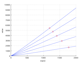
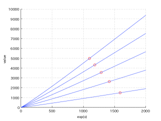
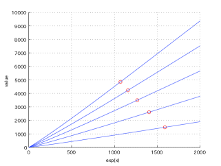
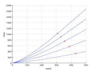
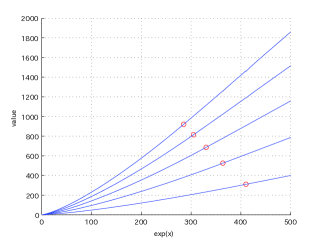
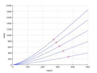
We now move on to the multiple-stage case. Using our randomization algorithm, the approximate value functions $\widetilde{v}^{(1)},\ldots,\widetilde{v}^{(5)}$ are computed for Erlang shape parameters $M=1,3$ and are shown in Figures 1 and 2, respectively, for $\gamma=0.02$ and $0.1$. The threshold levels $\widetilde{a}_{1}^{*},\ldots,\widetilde{a}_{5}^{*}$ (circles) are marked on the approximate value function curves. In particular, the top curve corresponds to the approximate value function $\widetilde{v}^{(5)}$. As expected, the thresholds are all above the strike $K=100$ and they admit the ordering $\widetilde{a}_{n+1}^{*}<\widetilde{a}_{n}^{*}$. This is consistent with Remark 2.1.

Recall that the process $\exp(-(\alpha-\gamma)t+X_{t})_{t\geq 0}$ is a martingale under the given parameters. Hence, for a small value of $\gamma$, the value function is close to linear in $\exp(x)$. On the other hand, as $\gamma$ increases, it appears to be more convex. Moreover, the function $\widetilde{v}^{(N)}$ decreases as $\gamma$ increases because $\gamma$ reduces the drift of $X$. As in the single stopping case, the difference between the value functions for $M=$ 1 and 3 is close to invisible. This suggests that these are reasonable approximations for the constant $\delta$ case. On the other hand, the optimal threshold levels show non-negligible difference between the cases $M=$ 1 and 3.

Case 1 (Exponential) with $M=1$	Case 1 (Exponential) with $M=3$
Case 2 (Weibull) with $M=1$	Case 2 (Weibull) with $M=3$
Case 3 (Folded Normal) with $M=1$	Case 3 (Folded Normal) with $M=3$

Figure 1. The approximate value functions when $\gamma=0.02$ with threshold levels $\widetilde{a}_{1}^{*},\ldots,\widetilde{a}_{5}^{*}$ (circles) marked on the approximate value function curves. The values are monotone in the number of stages (the top curve corresponds to the approximate value function $\widetilde{v}^{(5)}$).

Case 1 (Exponential) with $M=1$	Case 1 (Exponential) with $M=3$
Case 2 (Weibull) with $M=1$	Case 2 (Weibull) with $M=3$
Case 3 (Folded Normal) with $M=1$	Case 3 (Folded Normal) with $M=3$

Figure 2. The approximate value functions when $\gamma=0.1$.

5.3. Dependence on $N$ and $M$

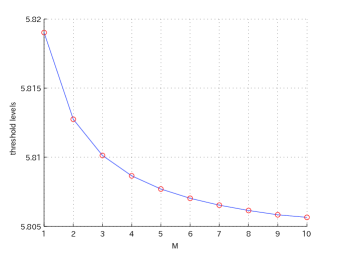
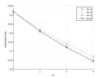
In Figure 3, we show the threshold levels with respect to the number of stages $N$ and to the Erlang shape parameter $M$ based on Case 3 with $\gamma=0.1$. On the left panel, we plot $\widetilde{a}^{*}_{1},\ldots,\widetilde{a}^{*}_{4}$ for fixed $M=1,\ldots,4$. Note that the first threshold $\widetilde{a}^{*}_{1}$ is independent of $M$. In the example on the right panel, we plot the threshold $\widetilde{a}^{*}_{2}$ over $M=1,\ldots,10$. As $M$ increases from $1$ to $10$, the threshold first decreases relatively fast within the narrow range $(5.81,5.82)$ for $M=1,2,3$, and then flattens toward the value 5.805 for larger $M$. Between $M=$ 9 and 10, the difference is well less than 0.001.

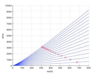
Figure 4 illustrates $\widetilde{v}^{(N)}$ for $N=1,\ldots,15$ with $\gamma=0.05$ and $M=1$. With more remaining exercise opportunities (large $N$), the function $\widetilde{v}^{(N)}$ is higher and the optimal threshold for the previous exercise is lower. We observe that the distance between successive optimal thresholds (marked by circles) reduces as the number of remaining exercises increases (see e.g. the top value function curve marked with 15 circles).

Figure 3. Dependence of the thresholds on $N$ and $M$ for Case 3 with $\gamma=0.1$. The left panel plots $\widetilde{a}^{*}_{1},\ldots,\widetilde{a}^{*}_{4}$ for fixed $M=1,\ldots,4$. The right panel plots the threshold $\widetilde{a}^{*}_{2}$ over $M=1,\ldots,10$.

Figure 4. Value functions and optimal thresholds (marked by circles) for Case 3 with $N=1,\ldots,15$ when $M=1$ and $\gamma=0.05$.

5.4. Limitations

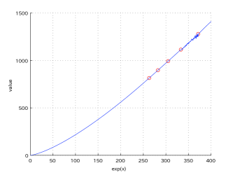
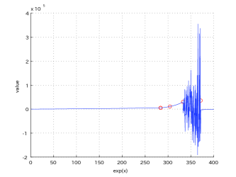
Recall from formula (4.9) for recovering the function $u^{(n,m)}$ from the parameter set $\Gamma=(A,B,C,D,E)$. In particular the coefficients $D$’s are multiplied by $\exp(\Phi(\alpha+M/\delta)x)x^{h}$, so this term tends to become very large near $\widetilde{a}_{1}^{*}$, even though $D$’s are zero above $\widetilde{a}_{1}^{*}$. From our numerical tests, it can take value up to the order of $10^{50}$ while the values of $D$’s tend to remain small. Recall that $p:=\alpha+M/\delta$ increases in $M$ and so does $\Phi(p)=\Phi(\alpha+M/\delta)$. In addition the maximum value of $h$ (the counting index in (4.9)) increases as $M$ and $N$ increase. As a result, the computation can break down when the Erlang shape parameter $M$ and/or the number of exercises $N$ are large. MATLAB or other softwares with double precision cannot handle the computation involving these large numbers.

Figure 5. Limitations: the value functions computed by MATLAB for Case 3 with $\gamma=0.1$ for $M=$4 (left), 5 (right).

In Figure 5, we plot the function $\widetilde{v}^{(N)}$ computed by MATLAB for Case 3 with $\gamma=0.1$ and $N=5$ for $M=4$ (left) and $M=5$ (right). While the parameters in $\Gamma$ can be computed instantly and do not explode, numerical imprecision in computing the value function may arise when small parameters are multiplied by very large numbers and summed up. Indeed, with $M=4$, discontinuities appear between $\widetilde{a}_{2}^{*}$ and $\widetilde{a}_{1}^{*}$, and with $M=5$ the error becomes visibly clear, yielding an inaccurate value function and threshold levels $\widetilde{a}^{*}$. This is consistent with the observation given in [28] (that deal with an American put option), where their randomization algorithm requires more than double precision. This issue can potentially be resolved by setting the machine epsilon as in [28] so as to increase precision. However, this is beyond the scope of our paper, because it requires special skills in computer science and it is our aim to evaluate the performance that can be achieved in a usual computing environment. Even given this potential limitation, the analytic formula is useful in its own right as it reveals the mathematical structure of the solution to the optimal multiple stopping problem.

This observation also highlights the potential trade-off between selecting large values of $M$ and $N$ given limits on machine precision. Nevertheless, we have seen from Tables 2 and 3 that the approximation remains stable for different small values of $M$. In summary, the analytic formula (4.9) is very useful and tractable for solving the optimal multiple stopping problem, as compared to the simulation approach.

Appendix A Proof of Proposition 4.1 and the updating formula

Fix $n\geq 1$ and $0\leq m\leq M-1$ and suppose (4.9), (4.11) and (4.12) hold. We shall show that the identity (4.18) can be written as (4.22) where the parameter set $\Gamma_{n,m+1}$ is given by (A.10) below.

First, for $\alpha<\beta$, straightforward integration gives the following expression for $\varpi_{l}^{(n,m)}$ as in (4.19).

(1) When $q=\Phi(p)$,

(A.1) $$\begin{split}\varpi_{l}^{(n,m)}(s,t,\Phi(p))&=A^{(n,m,l)}\frac{e^{-\Phi(p)s}-e^{-\Phi(p)t}}{\Phi(p)}+B^{(n,m,l)}\frac{e^{-(\Phi(p)-1)s}-e^{-(\Phi(p)-1)t}}{\Phi(p)-1}\\ &+\sum_{j\in\mathcal{I}_{p}}\sum_{h=0}^{I_{n,m}}e^{-(\Phi(p)+\xi_{j,p})s}s^{h}\sum_{g=h}^{I_{n,m}}C_{j,g}^{(n,m,l)}\frac{g!}{h!(\Phi(p)+\xi_{j,p})^{g+1-h}}\\ &-\sum_{j\in\mathcal{I}_{p}}\sum_{h=0}^{I_{n,m}}e^{-(\Phi(p)+\xi_{j,p})t}t^{h}\sum_{g=h}^{I_{n,m}}C_{j,g}^{(n,m,l)}\frac{g!}{h!(\Phi(p)+\xi_{j,p})^{g+1-h}}\\ &+\sum_{h=0}^{I_{n,m}}\frac{D_{h}^{(n,m,l)}}{h+1}(t^{h+1}-s^{h+1})+E^{(n,m,l)}\frac{e^{-(\Phi(p)-\Phi(\alpha))s}-e^{-(\Phi(p)-\Phi(\alpha))t}}{\Phi(p)-\Phi(\alpha)}.\end{split}$$

In particular, for $t=\infty$, if $\Phi(p)>1$ and $D^{(n,m,l)}=E^{(n,m,l)}=0$

(A.2) $$\begin{split}\varpi_{l}^{(n,m)}(s,\infty,\Phi(p))&=A^{(n,m,l)}\frac{e^{-\Phi(p)s}}{\Phi(p)}+B^{(n,m,l)}\frac{e^{-(\Phi(p)-1)s}}{\Phi(p)-1}\\ &+\sum_{j\in\mathcal{I}_{p}}\sum_{h=0}^{I_{n,m}}e^{-(\Phi(p)+\xi_{j,p})s}s^{h}\sum_{g=h}^{I_{n,m}}C_{j,g}^{(n,m,l)}\frac{g!}{h!(\Phi(p)+\xi_{j,p})^{g+1-h}}.\end{split}$$

(2) When $q=-\xi_{i,p}$, $\varpi_{l}^{(n,m)}(s,t,-\xi_{i,p})$ equals

(A.3) $$\begin{split}&A^{(n,m,l)}\frac{e^{\xi_{i,p}t}-e^{\xi_{i,p}s}}{\xi_{i,p}}+B^{(n,m,l)}\frac{e^{(\xi_{i,p}+1)t}-e^{(\xi_{i,p}+1)s}}{\xi_{i,p}+1}+\sum_{g=0}^{I_{n,m}}\frac{C_{i,g}^{(n,m,l)}}{g+1}(t^{g+1}-s^{g+1})\\ &+\sum_{j\in\mathcal{I}_{p}\backslash\{i\}}\sum_{h=0}^{I_{n,m}}e^{(\xi_{i,p}-\xi_{j,p})s}s^{h}\sum_{g=h}^{I_{n,m}}C_{j,g}^{(n,m,l)}\frac{g!}{h!(\xi_{j,p}-\xi_{i,p})^{g+1-h}}\\ &-\sum_{j\in\mathcal{I}_{p}\backslash\{i\}}\sum_{h=0}^{I_{n,m}}e^{(\xi_{i,p}-\xi_{j,p})t}t^{h}\sum_{g=h}^{I_{n,m}}C_{j,g}^{(n,m,l)}\frac{g!}{h!(\xi_{j,p}-\xi_{i,p})^{g+1-h}}\\ &+\sum_{j=0}^{I_{n,m}}\Big{[}e^{(\xi_{i,p}+\Phi(p))s}s^{j}-e^{(\xi_{i,p}+\Phi(p))t}t^{j}\Big{]}\sum_{h=j}^{I_{n,m}}D_{h}^{(n,m,l)}\frac{h!}{j!(-(\xi_{i,p}+\Phi(p)))^{h+1-j}}\\ &+E^{(n,m,l)}\frac{e^{(\xi_{i,p}+\Phi(\alpha))t}-e^{(\xi_{i,p}+\Phi(\alpha))s}}{\xi_{i,p}+\Phi(\alpha)}.\end{split}$$

In particular, if $s=-\infty$ and $A^{(n,m,l)}=B^{(n,m,l)}=C^{(n,m,l)}=0$,

(A.4) $$\varpi_{l}^{(n,m)}(-\infty,t,-\xi_{i,p})=-\sum_{j=0}^{I_{n,m}}e^{(\xi_{i,p}+\Phi(p))t}t^{j}\sum_{h=j}^{I_{n,m}}D_{h}^{(n,m,l)}\frac{h!}{j!(-(\xi_{i,p}+\Phi(p)))^{h+1-j}}+E^{(n,m,l)}\frac{e^{(\xi_{i,p}+\Phi(\alpha))t}}{\xi_{i,p}+\Phi(\alpha)}.$$

By letting $s=x$ and $t=\widetilde{a}^{*}_{L-1}$ and multiplying by $\exp(\Phi(p)x)$, we obtain

(A.5) $$e^{\Phi(p)x}\varpi_{L}(x,\widetilde{a}_{L-1}^{*},\Phi(p))=\hat{A}^{(n,m,L)}+\hat{B}^{(n,m,L)}e^{x}\\ +\sum_{i\in\mathcal{I}_{p}}\sum_{h=0}^{I_{n,m}+1}(\hat{C}^{(n,m,L)}_{i,h}e^{-\xi_{i,p}x}x^{h})+\sum_{h=0}^{I_{n,m}+1}(\hat{D}^{(n,m,L)}_{h}e^{\Phi(p)x}x^{h})+\hat{E}^{(n,m,L)}e^{\Phi(\alpha)x},$$

where

(A.6) $$\begin{split}\hat{A}^{(n,m,L)}&:={A^{(n,m,L)}}/{\Phi(p)},\;\hat{B}^{(n,m,L)}:={B^{(n,m,L)}}/{(\Phi(p)-1)},\\ \hat{C}^{(n,m,L)}_{i,h}&:=\sum_{g=h}^{I_{n,m}}C_{i,g}^{(n,m,L)}\frac{g!}{h!(\Phi(p)+\xi_{i,p})^{g+1-h}},\quad 0\leq h\leq I_{n,m},\quad\hat{C}^{(n,m,L)}_{i,I_{n,m}+1}:=0,\quad i\in\mathcal{I}_{p},\end{split}$$

and

(A.7) $$\begin{split}\hat{D}^{(n,m,L)}_{0}&:=1_{\{L\geq 2\}}\Big{[}\frac{-A^{(n,m,L)}e^{-\Phi(p)\widetilde{a}_{L-1}^{*}}}{\Phi(p)}+B^{(n,m,L)}\frac{-e^{-(\Phi(p)-1)\widetilde{a}_{L-1}^{*}}}{\Phi(p)-1}\\ &\qquad-\sum_{j\in\mathcal{I}_{p}}\sum_{h=0}^{I_{n,m}}e^{-(\Phi(p)+\xi_{j,p})\widetilde{a}_{L-1}^{*}}(\widetilde{a}_{L-1}^{*})^{h}\sum_{g=h}^{I_{n,m}}C_{j,g}^{(n,m,L)}\frac{g!}{h!(\Phi(p)+\xi_{j,p})^{g+1-h}}\\ &\qquad+\sum_{h=0}^{I_{n,m}}\frac{D_{h}^{(n,m,L)}}{h+1}(\widetilde{a}_{L-1}^{*})^{h+1}-\frac{E^{(n,m,L)}}{\Phi(p)-\Phi(\alpha)}e^{-(\Phi(p)-\Phi(\alpha))\widetilde{a}_{L-1}^{*}}\Big{]},\\ \hat{D}^{(n,m,L)}_{h}&:=-1_{\{L\geq 2\}}{D_{h-1}^{(n,m,L)}}/{h},\quad 1\leq h\leq I_{n,m}+1,\\ \hat{E}^{(n,m,L)}&:=1_{\{L\geq 2\}}{E^{(n,m,L)}}/{(\Phi(p)-\Phi(\alpha))}.\end{split}$$

Similarly, we have

(A.8) $$\sum_{i\in\mathcal{I}_{p}}\kappa_{i,p}e^{-\xi_{i,p}x}\varpi_{L}^{(n,m)}(\widetilde{a}_{L}^{*},x,-\xi_{i,p})=\check{A}^{(n,m,L)}+e^{x}\check{B}^{(n,m,L)}+\sum_{i\in\mathcal{I}_{p}}\sum_{h=0}^{I_{n,m}+1}e^{-\xi_{i,p}x}x^{h}\check{C}^{(n,m,L)}_{i,h}\\ +\sum_{h=0}^{I_{n,m}+1}e^{\Phi(p)x}x^{h}\check{D}^{(n,m,L)}_{h}+e^{\Phi(\alpha)x}\check{E}^{(n,m,L,i)},$$

where $\check{A}^{(n,m,L)}:=\sum_{i\in\mathcal{I}_{p}}\kappa_{i,p}{A^{(n,m,L)}}/{\xi_{i,p}}$, $\check{B}^{(n,m,L)}:=\sum_{i\in\mathcal{I}_{p}}\kappa_{i,p}{B^{(n,m,L)}}/{(\xi_{i,p}+1)}$,
$\check{C}^{(n,m,L)}_{j,h}:=\sum_{i\in\mathcal{I}_{p}}\kappa_{i,p}\check{C}^{(n,m,L,i)}_{j,h}$, $\check{D}^{(n,m,L)}_{h}:=\sum_{i\in\mathcal{I}_{p}}\kappa_{i,p}\check{D}^{(n,m,L,i)}_{h}$, $\check{E}^{(n,m,L)}:=\sum_{i\in\mathcal{I}_{p}}\kappa_{i,p}{E^{(n,m,L)}}/{(\xi_{i,p}+\Phi(\alpha))}$, with, for all $i\in\mathcal{I}_{p}$,

(A.9) $$\begin{split}\check{C}^{(n,m,L,i)}_{i,0}&:=-A^{(n,m,L)}\frac{e^{\xi_{i,p}\widetilde{a}_{L}^{*}}}{\xi_{i,p}}-B^{(n,m,L)}\frac{e^{(\xi_{i,p}+1)\widetilde{a}_{L}^{*}}}{\xi_{i,p}+1}-\sum_{g=0}^{I_{n,m}}\frac{C_{i,g}^{(n,m,L)}}{g+1}(\widetilde{a}_{L}^{*})^{g+1}\\ &\qquad+\sum_{j\in\mathcal{I}_{p}\backslash\{i\}}\sum_{h=0}^{I_{n,m}}(\widetilde{a}_{L}^{*})^{h}e^{(\xi_{i,p}-\xi_{j,p})\widetilde{a}_{L}^{*}}\sum_{g=h}^{I_{n,m}}C_{j,g}^{(n,m,L)}\frac{g!}{h!(\xi_{j,p}-\xi_{i,p})^{g+1-h}}\\ &\qquad+\sum_{j=0}^{I_{n,m}}\Big{[}e^{(\xi_{i,p}+\Phi(p))\widetilde{a}_{L}^{*}}(\widetilde{a}_{L}^{*})^{j}\Big{]}\sum_{h=j}^{I_{n,m}}D_{h}^{(n,m,L)}\frac{h!}{j!(-(\xi_{i,p}+\Phi(p)))^{h+1-j}}\\ &\qquad-E^{(n,m,L)}\frac{e^{(\xi_{i,p}+\Phi(\alpha))\widetilde{a}_{L}^{*}}}{\xi_{i,p}+\Phi(\alpha)},\\ \check{C}^{(n,m,L,i)}_{i,h}&:={C_{i,h-1}^{(n,m,L)}}/{h},\quad 1\leq h\leq I_{n,m}+1,\\ \check{C}^{(n,m,L,i)}_{j,h}&:=-\sum_{g=h}^{I_{n,m}}C_{j,g}^{(n,m,L)}\frac{g!}{h!(\xi_{j,p}-\xi_{i,p})^{g+1-h}},\quad 0\leq h\leq I_{n,m},\quad\check{C}^{(n,m,L,i)}_{j,I_{n,m}+1}:=0,\quad j\in\mathcal{I}_{p}\backslash\{i\},\\ \check{D}^{(n,m,L,i)}_{h}&:=-\sum_{g=h}^{I_{n,m}}D_{g}^{(n,m,L)}\frac{g!}{h!(-(\xi_{i,p}+\Phi(p)))^{g+1-h}},\quad 0\leq h\leq I_{n,m},\quad\check{D}^{(n,m,L,i)}_{I_{n,m}+1}:=0.\end{split}$$

Substituting (A.5) and (A.8) in (4.18), Proposition 4.1 is satisfied by setting $I_{n,m+1}=I_{n,m}+1$ and

(A.10) $$\begin{split}A^{(n,m+1,L)}&:=1_{\{L\leq n\}}(\Phi^{\prime}(p)\hat{A}^{(n,m,L)}+\check{A}^{(n,m,L)}),\\ B^{(n,m+1,L)}&:=1_{\{L\leq n\}}(\Phi^{\prime}(p)\hat{B}^{(n,m,L)}+\check{B}^{(n,m,L)}),\\ C^{(n,m+1,L)}_{i,0}&:=1_{\{L\leq n\}}\big{(}\Phi^{\prime}(p)\hat{C}_{i,0}^{(n,m,L)}+\check{C}_{i,0}^{(n,m,L)}+\kappa_{i,p}\sum_{L+1\leq l\leq n+1}\varpi_{l}^{(n,m)}(\widetilde{a}_{l}^{*},\widetilde{a}_{l-1}^{*},-\xi_{i,p})\big{)},\quad i\in\mathcal{I}_{p},\\ C^{(n,m+1,L)}_{i,h}&:=1_{\{L\leq n\}}(\Phi^{\prime}(p)\hat{C}_{i,h}^{(n,m,L)}+\check{C}_{i,h}^{(n,m,L)}),\quad 1\leq h\leq I_{n,m+1},\;i\in\mathcal{I}_{p},\\ D^{(n,m+1,L)}_{0}&:=1_{\{L\geq 2\}}\big{(}\Phi^{\prime}(p)\hat{D}_{0}^{(n,m,L)}+\check{D}_{0}^{(n,m,L)}+\Phi^{\prime}(p)\sum_{1\leq l\leq L-1}\varpi_{l}^{(n,m)}(\widetilde{a}_{l}^{*},\widetilde{a}_{l-1}^{*},\Phi(p))\big{)},\\ D^{(n,m+1,L)}_{h}&:=1_{\{L\geq 2\}}\big{(}\Phi^{\prime}(p)\hat{D}_{h}^{(n,m,L)}+\check{D}_{h}^{(n,m,L)}\big{)},\quad 1\leq h\leq I_{n,m+1},\\ E^{(n,m+1,L)}&:=1_{\{L\geq 2\}}(\Phi^{\prime}(p)\hat{E}^{(n,m,L)}+\check{E}^{(n,m,L)}).\end{split}$$

This completes the proof.

References

• [1] L. Alili and A. E. Kyprianou. Some remarks on first passage of Lévy processes, the American put and pasting principles. Annals of Applied Probability, 15(3):2062–2080, 2005.
• [2] S. Asmussen, F. Avram, and M. R. Pistorius. Russian and American put options under exponential phase-type Lévy models. Stochastic Processes and Their Applications, 109(1):79–111, 2004.
• [3] S. Asmussen, D. Madan, and M. Pistorius. Pricing equity default swaps under an approximation to the CGMY Lévy model. Journal of Computational Finance, 11(2):79–93, 2007.
• [4] S. Asmussen, O. Nerman, and M. Olsson. Fitting phase-type distributions via the EM algorithm. Scandinavian Journal of Statistics, 23:419–441, 1996.
• [5] S. Asmussen and J. Rosiński. Approximations of small jumps of Lévy processes with a view towards simulation. Journal of Applied Probability, 38(2):482–493, 2001.
• [6] F. Avram, A. E. Kyprianou, and M. R. Pistorius. Exit problems for spectrally negative Lévy processes and applications to (Canadized) Russion options. Annals of Applied Probability, 14:215–235, 2004.
• [7] F. Avram, Z. Palmowski, and M. R. Pistorius. On the optimal dividend problem for a spectrally negative Lévy process. Annals of Applied Probability, 17(1):156–180, 2007.
• [8] C. Bender. Dual pricing of multi-exercise options under volume constraints. Finance and Stochastics, 15:1–26, 2011.
• [9] F. Black. Interest rates as options. Journal of Finance, 50(5):1371–1376, 1995.
• [10] B. Bouchard, N. El Karoui, and N. Touzi. Maturity randomization for stochastic control problems. Annals of Applied Probability, 15:2575–2605, 2005.
• [11] N. Cai and L. Sun. Valuation of stock loans with jump risk. Journal of Economic Dynamics and Control, 2014. To appear.
• [12] R. Carmona and S. Dayanik. Optimal multiple stopping of linear diffusions. Mathematics of Operations Research, 33(2):446–460, 2008.
• [13] R. Carmona and N. Touzi. Optimal multiple stopping and valuation of swing options. Mathematical Finance, 18(2):239–268, 2008.
• [14] P. Carr. Randomization and the American put. Review of Financial Studies, 11:597–626, 1998.
• [15] N. Chiara, M. Garvin, and J. Vecer. Valuing simple multiple-exercise real options in infrastructure projects. Journal of Infrastructure Systems, 13(2):97–104, 2007.
• [16] S. Christensen and J. Lempa. Resolvent-techniques for multiple exercise problems. Applied Mathematical and Optimization, 71(1):95–123, 2015.
• [17] E. Dahlgren and T. Leung. An optimal multiple stopping approach to infrastructure investment decisions. Submitted, 2013.
• [18] M. Dai and Y.-K. Kwok. Optimal multiple stopping models of reload options and shout options. Journal of Economic Dynamics and Control, 32(7):2269 – 2290, 2008.
• [19] A. Dixit and R. Pindyck. Investment Under Uncertainty. Princeton University Press, 1994.
• [20] M. Egami, T. Leung, and K. Yamazaki. Default swap games driven by spectrally negative Lévy processes. Stochastic Processes and Their Applications, 123(2):347–384, 2013.
• [21] M. Egami and K. Yamazaki. Precautionary measures for credit risk management in jump models. Stochastics, 85(1):111–143, 2013.
• [22] M. Egami and K. Yamazaki. Phase-type fitting of scale functions for spectrally negative Lévy processes. Journal of Computational and Applied Mathematics, 264:1–22, 2014.
• [23] A. Ferreiro-Castilla, A. Kyprianou, R. Scheichla, and G. Suryanarayana. Multilevel Monte Carlo simulation for Lévy processes based on the Wiener-Hopf factorisation. Stochastic Processes and Their Applications, 124:985–1010, 2014.
• [24] M. Grasselli and V. Henderson. Risk aversion and block exercise of executive stock options. Journal of Economic Dynamics and Control, 33(1):109–127, 2009.
• [25] V. Henderson and D. Hobson. Optimal liquidation of derivative portfolios. Mathematical Finance, 21(3):365–382, 2011.
• [26] B. Hilberink and L. C. G. Rogers. Optimal capital structure and endogenous default. Finance and Stochastics, 6(2):237–263, 2002.
• [27] J. Jacod and A. N. Shiryaev. Limit theorems for stochastic processes, volume 288. Springer-Verlag, Berlin, second edition, 2003.
• [28] F. Kleinert and K. van Schaik. A variation of the Canadisation algorithm for the pricing of American options driven by Lévy processes. Working Paper, 2013.
• [29] M. Kobylanski, M.-C. Quenez, and E. Rouy-Mironescu. Optimal multiple stopping time problem. Annals of Applied Probability, 21(4):1365–1399, 2011.
• [30] A. Kuznetsov, A. Kyprianou, and V. Rivero. The theory of scale functions for spectrally negative Lévy processes. Springer Lecture Notes in Mathematics, 2061:97–186, 2013.
• [31] A. Kuznetsov, A. E. Kyprianou, J. C. Pardo, and K. van Schaik. A Wiener-Hopf Monte-Carlo simulation technique for Lévy processes. Annals of Applied Probability, 21:1749–1794, 2011.
• [32] A. E. Kyprianou. Introductory Lectures on Fluctuations of Lévy Processes with Applications. Universitext. Springer-Verlag, Berlin, 2006.
• [33] A. E. Kyprianou and Z. Palmowski. Distributional study of de Finetti’s dividend problem for a general Lévy insurance risk process. Journal of Applied Probability, 44(2):428–448, 2007.
• [34] A. E. Kyprianou and M. R. Pistorius. Perpetual options and Canadization through fluctuation theory. Annals of Applied Probability, 13(3):1077–1098, 2003.
• [35] A. E. Kyprianou and B. A. Surya. Principles of smooth and continuous fit in the determination of endogenous bankruptcy levels. Finance and Stochastics, 11(1):131–152, 2007.
• [36] T. Leung and M. Ludkovski. Optimal timing to purchase options. SIAM Journal on Financial Mathematics, 2(1):768–793, 2011.
• [37] T. Leung and M. Ludkovski. Accounting for risk aversion in derivatives purchase timing. Mathematics and Financial Economics, 6(4):363–386, 2012.
• [38] T. Leung and R. Sircar. Accounting for risk aversion, vesting, job termination risk and multiple exercises in valuation of employee stock options. Mathematical Finance, 19(1):99–128, 2009.
• [39] T. Leung and R. Sircar. Exponential hedging with optimal stopping and application to ESO valuation. SIAM Journal of Control and Optimization, 48(3):1422–1451, 2009.
• [40] T. Leung and K. Yamazaki. American step-up and step-down credit default swaps under Lévy models. Quantitative Finance, 13(1):137–157, 2013.
• [41] T. Leung, K. Yamazaki, and H. Zhang. Optimal multiple stopping with negative discount rate and random refraction times under Lévy models. Working paper, 2014.
• [42] S. Levendorskiı. Convergence of price and sensitivities in Carr’s randomization approximation globally and near barrier. SIAM Journal on Financial Mathematics, 2(1):79–111, 2011.
• [43] R. L. Loeffen. On optimality of the barrier strategy in de Finetti’s dividend problem for spectrally negative Lévy processes. Annals of Applied Probability, 18(5):1669–1680, 2008.
• [44] R. McDonald and D. Siegel. Investment and the valuation of firms when there is an option to shut down. International Economic Review, 26(2):331–349, 1985.
• [45] N. Meinshausen and B. Hambly. Monte Carlo methods for the valuation of multiple-exercise options. Mathematical Finance, 14, 2004.
• [46] E. Mordecki. Optimal stopping and perpetual options for Lévy processes. Finance and Stochastics, 6:473–493, 2002.
• [47] B. A. Surya and K. Yamazaki. Optimal capital structure with scale effects under spectrally negative Lévy models. International Journal of Theoretical and Applied Finance, 17(2), 2014.
• [48] H. G. Tucker. Absolute continuity of infinitely divisible distributions. Pacific J. Math, 12:1125–1129, 1962.
• [49] J. Xia and X. Zhou. Stock loans. Mathematical Finance, 17(2):307–317, 2007.
• [50] K. Yamazaki. Contraction options and optimal multiple-stopping in spectrally negative Lévy models. Applied Mathematics and Optimization, Forthcoming.
• [51] A. B. Zeghal and M. Mnif. Optimal multiple stopping and valuation of swing options in Lévy models. International Journal of Theoretical and Applied Finance, 9(8):1267–1297, 2006.