Parity measurement of remote qubits using dispersive coupling and photodetection

Abstract

Parity measurement is a key step in many entanglement generation and quantum error correction schemes. We propose a protocol for non-destructive parity measurement of two remote qubits, i.e., macroscopically separated qubits with no direct interaction. The qubits are instead dispersively coupled to separate resonators that radiate to shared photodetectors. The scheme is deterministic in the sense that there is no fundamental upper bound on the success probability. In contrast to previous proposals, our protocol addresses the scenario where number resolving photodetectors are available but the qubit–resonator coupling is time-independent and only dispersive.

I Introduction

One of the main challenges in quantum computing is that generally controlled qubit–qubit interactions should be strong while uncontrolled interactions should be negligible. Conceptually, the most straightforward approach to solving this issue is to physically remove uncontrolled degrees of freedom within a distance comparable to the qubit spacing, e.g., by trapping ions in ultra-high vacuum Cirac and Zoller (1995). An alternative approach is to entangle the qubits with photons that act as flying ancilla qubits. This approach allows placing the stationary qubits in remote locations because the photonic ancilla qubits generally interact weakly with the environment. In order to entangle the stationary qubits, the ancilla qubits only need to interfere optically with each other at detector inputs Cabrillo et al. (1999); Bose et al. (1999). Post-selection or local qubit operations conditioned on the detector outputs can then entangle the stationary qubits Cabrillo et al. (1999); Bose et al. (1999); Duan and Kimble (2003); Browne et al. (2003); Barrett and Kok (2005); Lim et al. (2005); Ladd et al. (2006); Busch et al. (2008); Matsuzaki et al. (2011); Azuma et al. (2012); Bernien et al. (2013); Bruschi et al. (2014). Such entanglement generation is at the heart of quantum repeaters and cluster-state models of quantum computing Briegel et al. (1998); Kok et al. (2007).

More generally, the photon-mediated approach allows performing a remote non-destructive parity measurement (RNPM) Azuma et al. (2012) described by the measurement operators $\hat{\Pi}_{1}=\left|gg\right\rangle\left\langle gg\right|+\left|ee\right\rangle\left\langle ee\right|$ and $\hat{\Pi}_{-1}=\left|ge\right\rangle\left\langle ge\right|+\left|eg\right\rangle\left\langle eg\right|$ for the even and odd parity outcomes, respectively. Here $\left|g\right\rangle$ and $\left|e\right\rangle$ are orthogonal single-qubit states that define the computational basis. Parity measurement is more general than entanglement generation in the sense that RNPM can generate entanglement without ancilla qubits, but protocols for preparing entangled states do not necessarily allow measuring parity without the use of ancilla qubits. Specifically, Bell pairs are generated from an initial product state $\left(\left|g\right\rangle+\left|e\right\rangle\right)\otimes\left(\left|g\right\rangle+\left|e\right\rangle\right)/2$ by measuring its parity, which provides just the right amount of information to produce maximally entangled pairs. However, we envision that the most useful application for ancilla-free RNPM may be in quantum error correction, where multi-qubit parity measurements are central to a wide variety of stabilizer codes Terhal (2015). Remote parity measurement in particular may prove useful in circumventing limitations that are inherent to codes that only use geometrically local parity checks Bravyi et al. (2010).

We note that the main challenge in non-destructive parity measurement is that the protocol must preserve coherence of arbitrary superpositions within the parity subspaces. In contrast, entanglement generation protocols drive the system into a known state and may assume a fixed initial state. In this sense RNPM is similarly challenging as applying a CPHASE gate to remote qubits Lim et al. (2005), although the two operations are not interchangeable without ancilla qubits.

We propose a protocol for RNPM that can be implemented in circuit quantum electrodynamics (cQED) Blais et al. (2004); Wallraff et al. (2004); Devoret and Schoelkopf (2013); Kelly et al. (2015) using standard and minimalistic resources, with the exception of number resolving photodetectors with high temporal resolution. Such detectors for itinerant microwave photons have not been realized to date but are under active theoretical and experimental development Romero et al. (2009); Chen et al. (2011); Peropadre et al. (2011); Fan et al. (2013); Hoi et al. (2013); Sathyamoorthy et al. (2014); Fan et al. (2014); Govenius et al. (2014); Gasparinetti et al. (2015); Koshino et al. (2015). In addition to the detectors, the requirements for our protocol are the following: a beam splitter, two qubit–resonator systems with dispersive coupling, coherent drive pulses applied to the resonators, and single-qubit phase gates conditioned on the recorded arrival times of the photons.

We emphasize that our protocol places few restrictions on the systems used as qubits. Specifically, we do not require $\Lambda$-type internal level structure to entangle the qubit state and a Fock state of the resonator, which is the typical starting point of most proposals for optical experiments Cabrillo et al. (1999); Bose et al. (1999); Duan and Kimble (2003); Browne et al. (2003); Barrett and Kok (2005); Lim et al. (2005); Busch et al. (2008); Bernien et al. (2013); Bruschi et al. (2014). Instead, our proposal works with a time-independent dispersive shift $\chi$ and resonator decay rate $\kappa$, both of which are standard features of cQED setups. The time-independent and dispersive qubit–resonator coupling gradually entangles the qubit state with coherent states of the resonator and continues to play an important role throughout the protocol. This is in contrast to the generation of single photons on demand in Ref. Lim et al. (2005), where the qubit state is entangled with Fock states effectively instantaneously compared to other time scales. However, if on-off modulation of $\chi$ is possible, we can use it to speed up the parity measurement by turning off the interaction at a specific time $t_{\textrm{off}}$ that maximizes the qubit–resonator entanglement. If the strong dispersive limit Schuster et al. (2007) $\chi\gg\kappa$ is also reached, the interaction becomes effectively instantaneous compared to other time scales ($t_{\textrm{off}}\ll\kappa^{-1}$). In this particular scenario, the protocol after $t_{\textrm{off}}$ reproduces a specific case of the protocol proposed by Azuma et al. in Ref. Azuma et al. (2012).

Kerckhoff et al. proposed another parity measurement protocol that relies on homodyne detection and sequential reflection of a probe signal from two resonators coupled to three-level atoms Kerckhoff et al. (2009). Roch et al. experimentally demonstrated the generation of odd-parity Bell states in cQED using a similar sequential setup, but with dispersive qubit–resonator coupling and three distinct outcomes Roch et al. (2014). The disadvantage of the latter scheme is that it distinguishes the even parity states from each other and therefore reveals too much to function as RNPM. Our protocol on the other hand measures both parities non-destructively in a non-sequential setup. This is possible because the photodetectors effectively erase the phase information that would allow distinguishing qubit states of the same parity. Instead, the photodetectors reveal the stochastic relative phase acquired by the states, which is the fundamental backaction of dispersive measurements Schuster et al. (2005); Gambetta et al. (2006, 2008). Conditioning phase gates on the photodetector outputs therefore allows undoing the measurement-induced dephasing within the parity subspaces, much like in the extensively studied case of a joint measurement of two qubits in a single resonator Lalumière et al. (2010); Tornberg and Johansson (2010); Riste et al. (2013).

The remainder of this article is organized as follows. Section II reviews measurement-induced dephasing and discusses its reversal in a single-qubit scenario. Section III introduces the RNPM protocol and demonstrates its validity under ideal conditions. It also suggests an alternative variation of the protocol for the strong dispersive limit and briefly discusses some practical hurdles to implementing the protocol. Section IV concludes the article.

II Reversing measurement-induced dephasing of a single qubit

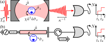
Figure 1: (Color online) (a) Schematic diagram of a qubit dispersively coupled to a resonator that radiates into a photodetector. At $t=0$, a short ($T_{\textrm{d}}\ll\kappa^{-1},\chi^{-1}$) external pulse drives the resonator mode ($\hat{a}$) from vacuum to a coherent state $\left|\alpha\right\rangle$. The resonator then evolves into a superposition of two coherent states at a rate $\chi$ due to a dispersive interaction that entangles the qubit ($\hat{\sigma}_{z}$) and the phase of the coherent state. At a rate $\kappa$, the resonator decays through a single port to an output mode monitored by a photodetector that encodes the arrival time $t_{i}$ of each photon in its output record $N\left(t\right)$. (b) The same setup depicted using cQED components. The optical cavity with asymmetric mirrors is replaced by a microwave transmission line resonator with asymmetric coupling capacitors. The free-space links are replaced by transmission lines. The circulator ensures that the photodetector causes no direct back-action on the system, even if the detector is not ideal.

Measurement-induced dephasing and the possibility of reversing it has been extensively discussed in the context of dispersive qubit measurement using quadrature detectors Schuster et al. (2005); Gambetta et al. (2006); Korotkov and Jordan (2006); Gambetta et al. (2008); Lalumière et al. (2010); Tornberg and Johansson (2010); Frisk Kockum et al. (2012); Riste et al. (2013); de Lange et al. (2014). The principle of reversing the dephasing using a photodetector has also been described by Frisk Kockum et al. in Ref. Frisk Kockum et al. (2012). Nevertheless, we begin by reviewing these concepts in a single-qubit scenario because it maps one-to-one to the even-parity subspace of the two-qubit scenario discussed in Sec. III.

We consider the qubit–resonator system illustrated in Fig. 1. We assume that the coupling is dispersive so that the closed-system Hamiltonian in the Schrödinger picture is well approximated by

$$\hat{H}_{\textrm{q-r}} =\hbar\left(\omega_{\textrm{r}}+\chi\hat{\sigma}_{z}\right)\hat{a}^{\dagger}\hat{a}+\frac{\hbar\tilde{\omega}_{\textrm{a}}}{2}\hat{\sigma}_{z}$$

$$\quad+\hbar\left[\varepsilon\left(t\right)e^{-i\omega_{\textrm{r}}t}\hat{a}^{\dagger}+\varepsilon^{*}\left(t\right)e^{i\omega_{\textrm{r}}t}\hat{a}\right],$$

as given in Ref. Gambetta et al. (2006). Here, $\hat{\sigma}_{z}=\left|e\right\rangle\left\langle e\right|-\left|g\right\rangle\left\langle g\right|$, $\hat{a}$ is the annihilation operator for photons in the resonator, $\omega_{\textrm{r}}/2\pi$ is the resonator frequency, $\tilde{\omega}_{\textrm{a}}/2\pi$ is the Lamb-shifted qubit frequency, $\chi/\pi$ is the dispersive frequency shift of the qubit per photon, and $\varepsilon\left(t\right)$ describes the amplitude of a classical drive of the resonator through a weakly-coupled port. However, we work in an interaction picture where we transform the basis states by $\mbox{exp}\left[i\left(\omega_{\textrm{r}}\hat{a}^{\dagger}\hat{a}+\tilde{\omega}_{\textrm{a}}\hat{\sigma}_{z}/2\right)t\right]$ and correspondingly redefine

$$\hat{H}_{\textrm{q-r}} =\hbar\chi\hat{\sigma}_{z}\hat{a}^{\dagger}\hat{a}+\hbar\left[\varepsilon\left(t\right)\hat{a}^{\dagger}+\varepsilon^{*}\left(t\right)\hat{a}\right].$$ (1)

We consider a drive that displaces the resonator from vacuum $\left|0\right\rangle$ into a coherent state $\left|\alpha\right\rangle=\hat{D}\left(\alpha\right)\left|0\right\rangle$ at $t=0$ but is otherwise off. This is approximately the case for a short but strong Gaussian pulse $\varepsilon\left(t\right)=i\alpha e^{-t^{2}/2T_{\textrm{d}}^{2}}/\sqrt{2\pi T_{\textrm{d}}^{2}}$, where $\kappa,\chi\ll T_{\textrm{d}}^{-1}\ll\omega_{\textrm{r}}$. We note that the average photon number $\left|\alpha\right|^{2}$ in the initial state is typically limited by assumptions underlying the dispersive coupling approximation Gambetta et al. (2006).

We assume that the dominant interaction between the qubit–resonator system and its environment is a weak linear coupling between the resonator and a transmission line with a photodetector at the other end. We assume that the photodetector emits negligible noise power to its input and that it is impedance matched, i.e., the detector is operated in the scattering mode Clerk et al. (2010). Given the rotating-wave, secular, and Born–Markov approximations, the corresponding stochastic master equation for the reduced density operator $\hat{\rho}_{I}\left(t\right)$ of the qubit–resonator system conditioned on the photodetector output is

$$d\hat{\rho}_{I} =dN\left(t\right)\mathcal{G}\left[\sqrt{\eta\kappa}\hat{a}\right]\hat{\rho}_{I}$$

$$\quad-dt\mathcal{H}\left[\frac{i}{\hbar}\hat{H}_{\textrm{q-r}}+\frac{\eta\kappa}{2}\hat{a}^{\dagger}\hat{a}\right]\hat{\rho}_{I}$$

$$\quad+dt\mathcal{D}\left[\sqrt{\left(1-\eta\right)\kappa}\hat{a}\right]\hat{\rho}_{I},$$ (2)

as given in Ref. Wiseman and Milburn (2010). Here, $\eta$ is the efficiency of the photodetector, $dN\left(t\right)\in\left\{0,1\right\}$ encodes the photon arrival times $T=\left\{t_{i}|dN\left(t_{i}\right)=1\right\}$, and $\left\langle dN\left(t\right)\right\rangle=dt\,\mbox{tr}\left[\eta\kappa\hat{a}^{\dagger}\hat{a}\hat{\rho}_{I}\right]$ gives the detection probability. The superoperator $\mathcal{H}\left[\hat{c}\right]\hat{\rho}=\hat{c}\hat{\rho}+\hat{\rho}\hat{c}^{\dagger}-\mbox{tr}\left[\hat{c}\hat{\rho}+\hat{\rho}\hat{c}^{\dagger}\right]\hat{\rho}$ describes the continuous evolution between detection events, $\mathcal{G}\left[\hat{c}\right]\hat{\rho}=\hat{c}\hat{\rho}\hat{c}^{\dagger}/\mbox{tr}\left[\hat{c}\hat{\rho}\hat{c}^{\dagger}\right]-\hat{\rho}$ accounts for the discrete jumps at $T$, and $\mathcal{D}\left[\hat{c}\right]\hat{\rho}=\hat{c}\hat{\rho}\hat{c}^{\dagger}-\frac{1}{2}\left(\hat{c}^{\dagger}\hat{c}\hat{\rho}+\hat{\rho}\hat{c}^{\dagger}\hat{c}\right)$ includes the effects of unmonitored decay. The subscript $I$ emphasizes that the solutions, called trajectories, depend on the stochastic photodetector output. In general, Eq. (2) should include terms corresponding to other imperfectly monitored decay channels, such as $\mathcal{D}\left[\sqrt{\mbox{$\gamma$}}\hat{\sigma}_{-}\right]\hat{\rho}_{I}$ describing spontaneous relaxation of the qubit, but we assume that $\kappa$ is sufficiently large to neglect them.

II.1 Unmonitored system: measurement-induced dephasing

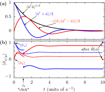
Figure 2: (Color online) Example trajectory (solid lines) and average evolution (dashed lines) of the qubit–resonator system (see Fig. 1) for $\chi=\kappa$, $\alpha=1$, and the qubit initially in $\left(\left|g\right\rangle+\left|e\right\rangle\right)/\sqrt{2}$. (a) Expectation values that are independent of the photon arrival times $T=\left\{t_{i}\right\}$: square root of the photon number $\hat{a}^{\dagger}\hat{a}$, the initially excited quadrature $\left(\hat{a}^{\dagger}+\hat{a}\right)/2$, and product of the conjugate quadrature $i\left(\hat{a}^{\dagger}-\hat{a}\right)/2$ and the qubit operator $-\hat{\sigma}_{z}$. Individually, $\left\langle\hat{a}^{\dagger}-\hat{a}\right\rangle=\left\langle\hat{\sigma}_{z}\right\rangle=0$ for all $t$ (not shown). (b) Expectation values of $\hat{\sigma}_{x}$ and $\hat{\sigma}_{y}$ which show decoherence of the qubit in the computational basis. The solid points at $t=10\kappa^{-1}$ show the state after applying a phase gate $\hat{R}\left(\phi\right)$ that reverses the measurement-induced dephasing $\phi\left(T\right)$ [see Eq. (8)]. The curves describe numerical solutions to Eqs. (3) and (7).

In the limit $\eta\rightarrow 0$, Eq. (2) reduces to the deterministic master equation

$$\partial_{t}\hat{\rho}=-\frac{i}{\hbar}\left[\hat{H}_{\textrm{q-r}},\hat{\rho}\right]+\mathcal{D}\left[\sqrt{\kappa}\hat{a}\right]\hat{\rho},$$ (3)

where we have dropped the subscript $I$ since the evolution is independent of the photodetector output. Furthermore, in the scattering mode the detector type is irrelevant for determining $\hat{\rho}$, and hence Eq. (3) is the same as for quadrature detection Gambetta et al. (2006); Wiseman and Milburn (2010).

Gambetta et al. solved Eq. (3) for a general drive $\varepsilon\left(t\right)$ Gambetta et al. (2006). For the specific parameters in our work, the solution can be expressed in closed form. For $t>0$, it is a superposition of two coherent resonator states entangled with the qubit state:

$$\hat{\rho}\left(t\right)=\sum_{i,j\in\left\{e,g\right\}}c_{ij}\left(t\right)\left|i\right\rangle\left\langle j\right|\otimes\left|\alpha_{i}\left(t\right)\right\rangle\left\langle\alpha_{j}\left(t\right)\right|,$$ (4)

where $\alpha_{g}=\alpha e^{\left(i\chi-\kappa/2\right)t}$ ($\alpha_{e}=\alpha e^{\left(-i\chi-\kappa/2\right)t}$) describes the exponentially decaying coherent resonator state given that the qubit is in $\left|g\right\rangle$ ($\left|e\right\rangle$) [see Fig. 2(a)]. The diagonal elements $c_{gg}$ and $c_{ee}$ remain at their initial values since there are no terms in Eq. (3) that flip $\left|g\right\rangle$ and $\left|e\right\rangle$. The off-diagonal elements decay according to $c_{eg}\left(t\right)=a_{eg}\left(t\right)/\left\langle\alpha_{g}\left(t\right)\left|\alpha_{e}\left(t\right)\right.\right\rangle$ and $c_{eg}\left(t\right)=c_{ge}^{*}\left(t\right)$, where $\left\langle\alpha_{g}\left(t\right)\left|\alpha_{e}\left(t\right)\right.\right\rangle=\mbox{exp}\left[-\left|\alpha\right|^{2}e^{-\kappa t}\left(1-e^{2i\chi t}\right)\right]$,

$$a_{eg}\left(t\right) =c_{eg}\left(0\right)\mbox{exp}\left[-2i\chi\int_{0}^{t}\alpha_{e}\left(t^{\prime}\right)\alpha_{g}^{*}\left(t^{\prime}\right)dt^{\prime}\right]$$

$$=c_{eg}\left(0\right)\mbox{exp}\left[-\left|\alpha\right|^{2}\frac{1-e^{\left(2i\chi-\kappa\right)t}}{1-i\kappa/2\chi}\right],$$ (5)

and $c_{eg}\left(0\right)$ is the initial value of the off-diagonal element.

Here $\left|c_{eg}\left(t\right)\right|$ quantifies the phase coherence remaining in the qubit–resonator system as a whole, while $2a_{eg}\left(t\right)=\left\langle\hat{\sigma}_{x}\left(t\right)\right\rangle-i\left\langle\hat{\sigma}_{y}\left(t\right)\right\rangle$ describes the lateral components of the qubit Bloch vector after tracing out the resonator [see Fig. 2(b)]. For $t\gg\kappa^{-1}$, the two are equivalent because the resonator state approaches vacuum exponentially irrespective of the qubit state. Furthermore, in the long time limit $c_{eg}\left(t\right)/c_{eg}\left(0\right)\approx\mbox{exp}\left[-\left|\alpha\right|^{2}/\left(1-i\kappa/2\chi\right)\right]$ so the net effect of the process on the qubit consists of a coherent rotation by an angle

$$\phi_{\textnormal{uncond}}=-\left|\alpha\right|^{2}/\left(2\chi/\kappa+\kappa/2\chi\right)$$ (6)

together with a reduction of coherence by a factor of $\mbox{exp}\left[-\left|\alpha\right|^{2}/\left(1+\kappa^{2}/4\chi^{2}\right)\right]$. The latter is called measurement-induced dephasing because it is directly related to the ability to determine the qubit state by monitoring the radiation leaking out of the system Gambetta et al. (2006, 2008).

II.2 Reversing dephasing using a photodetector

In the opposite limit of perfect photodetection ($\eta\rightarrow 1$), Eq. (2) reduces to

$$d\hat{\rho}_{I} =dN\left(t\right)\mathcal{G}\left[\sqrt{\kappa}\hat{a}\right]\hat{\rho}_{I}$$

$$\quad-dt\mathcal{H}\left[\frac{i}{\hbar}\hat{H}_{\textrm{q-r}}+\frac{\kappa}{2}\hat{a}^{\dagger}\hat{a}\right]\hat{\rho}_{I},$$ (7)

which does not include any unmonitored decay channels and therefore does not change the purity of the initial state Wiseman and Milburn (2010). Since the purity does not change and there are no terms that flip $\left|g\right\rangle$ and $\left|e\right\rangle$, the initial qubit state must be restored in the long-time limit by a phase gate

$$\hat{R}\left(\phi\right)=e^{-i\phi/2}\left|g\right\rangle\left\langle g\right|+e^{i\phi/2}\left|e\right\rangle\left\langle e\right|,$$

where $\phi$ is determined by solving Eq. (7) for a given $dN\left(t\right)$. Below, we show that this stochastic phase is independent of the initial qubit state and can be written in closed form as

$$\phi\left(T\right)=2\chi\sum_{t_{i}\in T}t_{i}.$$ (8)

Equation (8) can be intuitively understood by noting that the photons are all injected into the resonator at $t=0$, and hence the time each detected photon interacts with the qubit is equal to $t_{i}$. The contributions add linearly so the total accumulated dispersive phase shift between $\left|e\right\rangle$ and $\left|g\right\rangle$ is $\sum_{i}2\chi t_{i}$, as shown below for a pure initial state. Frisk Kockum et al. used an alternative method of solving the problem by applying a polaron transformation that allows writing a stochastic master equation for a two-level system only Frisk Kockum et al. (2012). Specifically, choosing $\eta=1$, $\epsilon_{m}t_{\textnormal{meas}}=i\alpha$, and $t_{\textnormal{meas}}\ll\chi^{-1},\kappa^{-1}$ for the parameters defined in Ref. Frisk Kockum et al. (2012) corresponds to the scenario we consider. Note, however, that the analysis in Ref. Frisk Kockum et al. (2012) excludes the coherent evolution due to the ac Stark shift $2\chi\textnormal{Re}\left(\alpha_{g}\alpha_{e}^{\star}\right)$. Compared to our results, this leads to an additional phase factor that approaches $\mbox{exp}\left(-i\phi_{\textnormal{uncond}}\right)$ for $t\gg\kappa^{-1}$ (see Eq. (26) in Ref. Frisk Kockum et al. (2012)).

For a pure initial state, Eq. (7) for the density operator $\hat{\rho}_{I}=\left|\psi_{I}\right\rangle\left\langle\psi_{I}\right|$ is equivalent to a stochastic Schrödinger equation for an unnormalized state $\left|\psi_{I}^{\prime}\left(t\right)\right\rangle=\left\langle\psi_{I}^{\prime}\left(t\right)\left|\psi_{I}^{\prime}\left(t\right)\right.\right\rangle^{1/2}\left|\psi_{I}\right\rangle$ Wiseman and Milburn (2010). For $t>0$, this means solving the Schrödinger equation for a non-Hermitian Hamiltonian $\hbar\left(\chi\hat{\sigma}_{z}-i\kappa/2\right)\hat{a}^{\dagger}\hat{a}$ between detection events, while a detected photon is taken into account by applying the jump operator $\hat{a}$ and renormalizing the resulting state. A photon is detected whenever $\left\langle\psi_{I}^{\prime}\left(t\right)\left|\psi_{I}^{\prime}\left(t\right)\right.\right\rangle$ reaches a random number $r_{i}$ drawn uniformly and independently from $\left[0,1\right]$ for each detection event $i$.

For a normalized initial state $\left(q_{g}\left|g\right\rangle+q_{e}\left|e\right\rangle\right)\left|\alpha\right\rangle$, the unnormalized state before the first detection event is

$$\left|\psi_{I}^{\prime}\left(t\right)\right\rangle =e^{-\left|\alpha\right|^{2}\left(1-e^{-\kappa t}\right)/2}\left(q_{g}\big{|}g\big{\rangle}\big{|}\alpha e^{\left(i\chi-\kappa/2\right)t}\big{\rangle}\right.$$

$$\quad\quad\quad\quad\quad\quad\quad\quad\,\,\,+\left.q_{e}\big{|}e\big{\rangle}\big{|}\alpha e^{\left(-i\chi-\kappa/2\right)t}\big{\rangle}\right).$$

If $r_{1}>e^{-\left|\alpha\right|^{2}}$, a photon is detected at $t_{1}=-\kappa^{-1}\ln\left[1+\left|\alpha\right|^{-2}\ln\left(r_{1}\right)\right]$ and the normalized state after applying $\hat{a}$ becomes

$$q_{g}e^{i\chi t_{1}}\big{|}g\big{\rangle}\big{|}\alpha e^{\left(i\chi-\kappa/2\right)t}\big{\rangle}+q_{e}e^{-i\chi t_{1}}\big{|}e\big{\rangle}\big{|}\alpha e^{\left(-i\chi-\kappa/2\right)t}\big{\rangle}.$$

Similarly, each subsequent detection event results in factors of $e^{\pm i\chi t_{i}}$, leading to the normalized state

$$\left|\psi_{I}\left(t\right)\right\rangle =q_{g}\exp\left[i\chi\sum_{t_{i}<t}t_{i}\right]\left|g\right\rangle\left|\alpha e^{(i\chi-\kappa/2)t}\right\rangle$$

$$\quad+q_{e}\exp\left[-i\chi\sum_{t_{i}<t}t_{i}\right]\left|e\right\rangle\left|\alpha e^{(-i\chi-\kappa/2)t}\right\rangle,$$

where $t_{i}\in T$ and no more jumps occur when $r_{i}<\exp\left(-\left|\alpha\right|^{2}e^{-\kappa t_{i-1}}\right)$, with $t_{0}=0$. See Fig. 2(b) for an example with one detection event.

Evidently applying $\hat{R}\left[\phi\left(T|t_{i}<t\right)\right]$ to $\left|\psi_{I}\left(t\right)\right\rangle$ undoes the relative phase between the $\left|g\right\rangle$ and $\left|e\right\rangle$ terms above. In the long-time limit $t\gg\kappa^{-1}\log\left|\alpha\right|$, the overlap $\left|\left\langle\psi_{I}\left(0\right)\left|\hat{R}\left(\phi\right)\right|\psi_{I}\left(t\right)\right\rangle\right|$ furthermore approaches unity and additional detection events become exponentially unlikely as the resonator returns to $\left|0\right\rangle$. Therefore we conclude that the combination of photodetection and $\hat{R}\left(\phi\right)$ effectively erases all the information that leaked out of the qubit during the process. In the parity measurement protocol, the same principle is used to erase only the part of the information that would allow distinguishing between $\left|gg\right\rangle$ and $\left|ee\right\rangle$ if a different scattering-mode detection scheme were used.

Note that the resonator and the qubit periodically return to a product state, i.e., $\alpha_{g}\left(\tilde{t}_{k}\right)=\alpha_{e}\left(\tilde{t}_{k}\right)=\left(-1\right)^{k}e^{-\kappa\tilde{t}_{k}/2}$ for all $\tilde{t}_{k}\in\left\{k\pi\chi^{-1}|k\in\mathbb{Z}^{+}\right\}$ [see Fig. 2(a)]. At these times the dynamics can be stopped by a second displacement $\hat{D}\left[-\alpha_{g}\left(\tilde{t}_{k}\right)\right]$ that brings the resonator to $\left|0\right\rangle$ deterministically, thereby decoupling the duration of the measurement from $\kappa^{-1}$ in the $\chi\apprge\kappa$ regime. We take advantage of this possibility in the parity measurement protocol proposed in the next section.

III Remote Parity Measurement

Figure 3 shows the setup we propose for measuring the parity $\hat{\sigma}_{z,1}\hat{\sigma}_{z,2}$ of two remote qubits. It consists of two identical instances of the dispersively coupled qubit–resonator system described in the previous section. The two resonator modes $\hat{a}_{1}$ and $\hat{a}_{2}$ are driven to an identical coherent state $\left|\alpha\right\rangle$ at $t=0$ but the radiation leaking out of them is not measured individually. Rather, a 50:50 beam splitter is arranged such that two identical photodetectors monitor the sum and difference modes with lowering operators $\hat{c}_{\pm}=\left(\hat{a}_{1}\pm\hat{a}_{2}\right)/\sqrt{2}$. The stochastic master equation for this system is

$$d\hat{\rho}_{I} =dN_{+}\left(t\right)\mathcal{G}\left[\sqrt{\eta\kappa}\hat{c}_{+}\right]\hat{\rho}_{I}$$

$$\quad+dN_{-}\left(t\right)\mathcal{G}\left[\sqrt{\eta\kappa}\hat{c}_{-}\right]\hat{\rho}_{I}$$

$$\quad-dt\mathcal{H}\left[\frac{i}{\hbar}\hat{H}_{\textrm{q-r}}^{(2)}+\frac{\eta\kappa}{2}\hat{c}_{+}^{\dagger}\hat{c}_{+}+\frac{\eta\kappa}{2}\hat{c}_{-}^{\dagger}\hat{c}_{-}\right]\hat{\rho}_{I}$$

$$\quad+dt\mathcal{D}\left[\sqrt{\left(1-\eta\right)\kappa}\hat{c}_{+}\right]\hat{\rho}_{I}$$

$$\quad+dt\mathcal{D}\left[\sqrt{\left(1-\eta\right)\kappa}\hat{c}_{-}\right]\hat{\rho}_{I},$$ (9)

where $\eta$ is the photodetection efficiency, $N_{\pm}\left(t\right)$ is the number of photons registered by the detector monitoring $\hat{c}_{\pm}$, and

$$\hat{H}_{\textrm{q-r}}^{(2)}=\hbar\chi\left(\hat{\sigma}_{z,1}\hat{a}_{1}^{\dagger}\hat{a}_{1}+\hat{\sigma}_{z,2}\hat{a}_{2}^{\dagger}\hat{a}_{2}\right)$$ (10)

for $t>0$. We denote coherent states of the sum and difference modes by $\left|\beta\right\rangle_{\pm}$.

The parity measurement and the measurement-induced dephasing in this scenario are closely connected to the case of multiple qubits coupled to the same resonator mode Hutchison et al. (2009); Bishop et al. (2009); Helmer and Marquardt (2009); Lalumière et al. (2010); Tornberg and Johansson (2010); Riste et al. (2013); Frisk Kockum et al. (2012); Nigg and Girvin (2013); Govia et al. (2015). Within the even-parity subspace, the difference mode in fact remains in vacuum so, mathematically, the description of the system maps one-to-one to the single resonator case. However, physically the situation is distinct because the populated resonator mode is the non-local sum mode. In the odd-parity subspace neither mode remains in vacuum.

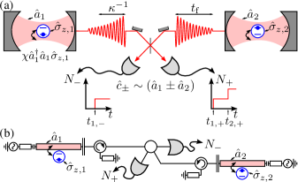
Figure 3: (Color online) (a) Schematic setup for measuring the parity $\hat{\sigma}_{z,1}\hat{\sigma}_{z,2}$ of two qubits located in identical resonators (see also Fig. 1). The resonators are driven into a coherent state $\left|\alpha\right\rangle$ at $t=0$ after which their phase becomes entangled with the local qubit at a rate $\chi$. At a rate $\kappa$, the resonators radiate into a 50:50 beam splitter with photodetectors monitoring the output modes. The relative phases are chosen such that the detectors monitor $\hat{c}_{\pm}=\left(\hat{a}_{1}\pm\hat{a}_{2}\right)/\sqrt{2}$. At a final time $t_{\textrm{f}}$ (integer multiple of $\pi\chi^{-1}$) the resonators are displaced back to vacuum. Recording more than zero photons for $\hat{c}_{-}$ [$N_{-}\left(t_{\textrm{f}}\right)>0$] indicates odd parity with certainty while $N_{-}\left(t_{\textrm{f}}\right)=0$ partially projects the qubits to the even-parity subspace. The final $N_{-}\left(t_{\textrm{f}}\right)$ is sufficient for reversing measurement-induced dephasing within the odd-parity subspace but the full time-resolved $N_{+}\left(t\right)$ is needed in the even-parity case. (b) The same setup depicted using cQED components. The beam splitter is replaced by a $180^{\circ}$ hybrid coupler.

III.1 Protocol

In this section, we describe the proposed RNPM protocol and its effect on the qubits. Section III.2 proves the validity of these claims analytically for $\eta\rightarrow 1$. Additionally, Appendix A presents some numerical trajectories in non-ideal cases.

The steps of the protocol are the following:

1. Start with the resonators in $\left|0\right\rangle$ and the qubits in an arbitrary pure state

   $$\left|\psi_{\textrm{q}}\left(0\right)\right\rangle=\sum_{i,j\in\left\{e,g\right\}}q_{ij}\left|ij\right\rangle.$$ (11)

2. Apply $\hat{D}\left(\alpha\right)$ to both resonators at $t=0$.

3. Wait until $t_{\textrm{f}}=k\pi\chi^{-1}$, where $k\in\mathbb{\mathbb{Z}}^{+}$ is arbitrary.

4. Apply $\hat{D}\left[-\left(-1\right)^{k}\alpha e^{-\kappa t_{\textrm{f}}/2}\right]$ to both resonators.

5. Compute the measurement induced phases

   $$\phi_{+} =2\chi\sum_{t_{i}\in T_{+}}t_{i}$$ (12)

   $$\textnormal{and }\phi_{-} =\pi N_{-}\left(t_{\textrm{f}}\right),$$ (13)

   and apply the local qubit feedback operations

   $$\hat{F} =\hat{R}\left(\frac{\phi_{+}}{2}+\frac{\phi_{-}}{2}\right)\otimes\hat{R}\left(\frac{\phi_{+}}{2}-\frac{\phi_{-}}{2}\right).$$ (14)

Assuming $\eta\rightarrow 1$, the state of the qubits after these steps is

$$\left|\psi_{\textrm{q}}\left(t_{\textrm{f}}\right)\right\rangle=\left[\sqrt{P_{-1}}\hat{\Pi}_{-1}+\sqrt{P_{1}}\hat{\Pi}_{1}\right]\left|\psi_{\textrm{q}}\left(0\right)\right\rangle,$$ (15)

where $P_{1}=1-P_{-1}$. The outcome of the parity measurement is indicated by $P_{-1}=\left\langle\psi_{\textrm{q}}\left(t_{\textrm{f}}\right)\left|\hat{\Pi}_{-1}\right|\psi_{\textrm{q}}\left(t_{\textrm{f}}\right)\right\rangle$ and is determined by $N_{-}\left(t_{\textrm{f}}\right)$ and $T_{+}=\left\{t_{i}|dN_{+}\left(t_{i}\right)=1\right\}$ according to

$$P_{-1}=\begin{cases}1\quad\mbox{if }N_{-}\left(t_{\textrm{f}}\right)>0\\ \left(\left|q_{ge}\right|^{2}+\left|q_{eg}\right|^{2}\right)\left({\displaystyle\prod_{t_{i}\in T_{+}}\cos\chi t_{i}}\right)^{2}&\mbox{otherwise.}\end{cases}$$

Evidently a single $\hat{c}_{-}$ detection event leads to complete parity projection to the odd-parity subspace ($\left\langle\hat{\sigma}_{z,1}\hat{\sigma}_{z,1}\right\rangle=-1$), while $\hat{c}_{+}$ detections in general lead to an exponential suppression of the odd-parity components, as shown in Fig. 4. Therefore the outcome of the protocol is not strictly speaking binary, but rather continuous in the interval $P_{-1}\in[0,1]$. However, in the limit of many photodetection events, the protocol is well approximated by a projective parity measurement with $P_{-1}\in\left\{0,1\right\}$, up to exponentially small corrections given by the exact result. The expected number of detected photons is $\left|\alpha\right|^{2}\left(1-e^{-\kappa t_{\textrm{f}}}\right)$ and therefore tunable. Furthermore, if $P_{-1}$ is not sufficiently close to zero or one at $t_{\textrm{f}}$, steps 2 through 4 of the protocol can be repeated arbitrarily many times at the expense of increased operation time. In that case, a single feedback operation $\hat{F}$ applied after the last repetition should account for all detected photons. The displacements in steps 4 and 2 of adjacent repetitions can be combined into a single operation as well.

Finally, we claim that the outcome probabilities are distributed according to the parity of the initial state. More specifically, the ensemble average of $P_{-1}$ is $\textnormal{E}\left[P_{-1}\right]=\left\langle\psi_{\textrm{q}}\left(0\right)\left|\hat{\Pi}_{-1}\right|\psi_{\textrm{q}}\left(0\right)\right\rangle$. This implies that the protocol is indeed a parity measurement, rather than some other operation that leads to a well-defined parity.

III.2 Full temporal evolution

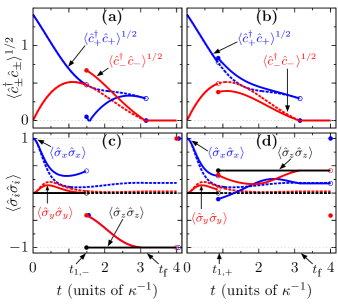
Figure 4: (Color online) Example trajectories (solid lines) and average evolution (dashed lines) for the two-qubit setup shown in Fig. 3 with $\chi=\kappa$, $\alpha=1$, $t_{\textrm{f}}=\pi\chi^{-1}$, and the qubits initially in $\left(\left|g\right\rangle+\left|e\right\rangle\right)^{\otimes 2}/2$. The left column (a,c) shows a trajectory that leads to projection of the qubits into the odd-parity subspace, while the right column (b,d) shows partial projection into the even-parity subspace. (a,b) The expected photodetection rates in units of $\kappa$ for the sum and difference modes ($\hat{c}_{\pm}$), with $t_{1,\pm}$ indicating the first and only photodetection event in the selected trajectories. Up to $t_{\textrm{f}}$, the local field quadratures $\left\langle\hat{a}_{j}^{\dagger}+\hat{a}_{j}\right\rangle/2$ and $-i\hat{\sigma}_{z,j}\left\langle\hat{a}_{j}^{\dagger}-\hat{a}_{j}\right\rangle/2$ are identical to those shown in Fig. 2(a), regardless of detection events. (c,d) Expectation values of the Bell state stabilizers $\hat{\sigma}_{i,1}\hat{\sigma}_{i,2}$, where $i\in\left\{x,y,z\right\}$. A projective parity measurement of the specified initial state leads to $\left\langle\hat{\sigma}_{z,1}\hat{\sigma}_{z,2}\right\rangle=\pm 1$ and conserves $\left\langle\hat{\sigma}_{x,1}\hat{\sigma}_{x,2}\right\rangle=1$. The solid points at $t=4\kappa^{-1}$ show the state after applying a phase gate $\hat{F}$ [see Eq. (14)] that reverses the measurement-induced dephasing, i.e., restores $\left\langle\hat{\sigma}_{x,1}\hat{\sigma}_{x,2}\right\rangle=1$. The curves describe numerical solutions to Eqs. (9) and (16) with $\eta=1$. Overlapping points have been offset horizontally for clarity.

Let us first give a qualitative explanation for Eqs. (12)–(15) by rewriting the Hamiltonian in Eq. (10) in the basis of the monitored operators as

$$\hat{H}_{\textrm{q-r}}^{(2)} =\frac{\hbar\chi}{2}\left[(\hat{\sigma}_{z,1}+\hat{\sigma}_{z,2})(\hat{c}_{+}^{\dagger}\hat{c}_{+}+\hat{c}_{-}^{\dagger}\hat{c}_{-})\right.$$

$$\qquad\quad\left.+(\hat{\sigma}_{z,1}-\hat{\sigma}_{z,2})(\hat{c}_{+}^{\dagger}\hat{c}_{-}+\hat{c}_{+}\hat{c}_{-}^{\dagger})\right].$$

Note that after the initial displacements the sum and difference modes start in $\left|\sqrt{2}\alpha\right\rangle_{+}$ and $\left|0\right\rangle_{-}$, respectively. Furthermore, there are no terms in Eq. (9) that flip the qubits in the computational basis so parity is conserved if it is initially well defined. For an even-parity initial state, $\hat{\sigma}_{z,1}-\hat{\sigma}_{z,2}$ yields zero so there are no terms in Eq. (9) that excite the difference mode out of $\left|0\right\rangle_{-}$ and we can therefore trace it out without loss of information. The remaining terms are identical to the single qubit case [see Eq. (7)] with the mapping $\left|gg\right\rangle\rightarrow\left|g\right\rangle$, $\left|ee\right\rangle\rightarrow\left|e\right\rangle$, and $\hat{c}_{+}\rightarrow\hat{a}$. This explains why Eq. (12) matches Eq. (8). On the other hand for an odd-parity initial state, $\hat{\sigma}_{z,1}+\hat{\sigma}_{z,2}$ yields zero so the dispersive $\hat{c}_{\pm}^{\dagger}\hat{c}_{\pm}$ terms in $\hat{H}_{\textrm{q-r}}^{(2)}$ vanish. Instead, photons are exchanged between the two bosonic modes by the $\hat{c}_{\pm}^{\dagger}\hat{c}_{\mp}$ terms with a phase flip between $\left|ge\right\rangle$ and $\left|eg\right\rangle$ associated with each exchange. Since the only other event that changes the photon number in $\hat{c}_{-}$ is a detection event $dN_{-}=1$, the parity of $N_{-}\left(t_{\textrm{f}}\right)$ and the parity of the number of phase flips must match given that $\hat{c}_{-}$ starts and ends in vacuum and $\eta=1$. This explains Eq. (13).

Let us formally prove the validity of Eqs. (12)–(15) and the associated probabilities for a pure initial state by explicitly solving the stochastic Schrödinger equation corresponding to Eq. (9) in the $\eta\rightarrow 1$ limit. Analogously to the single-qubit case, the jump operators are $\hat{c}_{\pm}$ and the non-Hermitian Hamiltonian that determines the evolution of the unnormalized state $\left|\psi_{I}^{\prime}\left(t\right)\right\rangle$ is

$$H^{\prime} =\hat{H}_{\textrm{q-r}}^{(2)}-i\hbar\frac{\kappa}{2}\left(\hat{c}_{+}^{\dagger}\hat{c}_{+}+\hat{c}_{-}^{\dagger}\hat{c}_{-}\right)$$

$$=\sum_{j=1}^{2}\hbar\left(\chi\hat{\sigma}_{z,j}-i\hbar\frac{\kappa}{2}\right)\hat{a}_{j}^{\dagger}\hat{a}_{j}$$

for $t>0$. A photon is detected whenever $\left\langle\psi_{I}^{\prime}\left(t\right)\left|\psi_{I}^{\prime}\left(t\right)\right.\right\rangle$ reaches a random number $r_{i}$ drawn uniformly and independently from $\left[0,1\right]$ for each event $i$. The detector that clicks is chosen at random with probabilities weighted by $\big{\langle}\psi_{I}^{\prime}\left(t\right)\big{|}\hat{c}_{\pm}^{\dagger}\hat{c}_{\pm}\big{|}\psi_{I}^{\prime}\left(t\right)\big{\rangle}$.

For the initial state given in Eq. (11), the unnormalized state $\left|\psi_{I}^{\prime}\left(t\right)\right\rangle$ before the first detection event is

$$e^{-\left|\alpha\right|^{2}\left(1-e^{-\kappa t}\right)} \left(q_{gg}\big{|}gg\big{\rangle}\big{|}Ae^{i\chi t}\big{\rangle}_{+}\big{|}0\big{\rangle}_{-}\right.$$

$$\,\,+q_{ee}\big{|}ee\big{\rangle}\big{|}Ae^{-i\chi t}\big{\rangle}_{+}\big{|}0\big{\rangle}_{-}$$

$$\,\,+q_{ge}\big{|}ge\big{\rangle}\big{|}A\cos\chi t\big{\rangle}_{+}\big{|}iA\sin\chi t\big{\rangle}_{-}$$

$$\,\,+\left.q_{eg}\big{|}eg\big{\rangle}\big{|}A\cos\chi t\big{\rangle}_{+}\big{|}-iA\sin\chi t\big{\rangle}_{-}\right),$$

where $A\left(t\right)=\sqrt{2}\alpha e^{-\kappa t/2}$ is an exponentially decaying amplitude of the remaining radiation. If $r_{1}>\exp\left[-2\left|\alpha\right|^{2}\left(1-e^{-\kappa t_{\textrm{f}}}\right)\right]$, a photon is detected at $t_{1}=-\kappa^{-1}\ln\left[1+\left|\alpha\right|^{-2}\ln\left(r_{1}\right)/2\right]$ and the state $\left|\psi_{I}\left(t\right)\right\rangle$ after the event is proportional to

$$iq_{ge}\big{|}ge\big{\rangle}\big{|}A\cos\chi t\big{\rangle}_{+}\big{|}iA\sin\chi t\big{\rangle}_{-}$$

$$+ \left(-i\right)q_{eg}\big{|}eg\big{\rangle}\big{|}A\cos\chi t\big{\rangle}_{+}\big{|}-iA\sin\chi t\big{\rangle}_{-}$$

if $dN_{-}\left(t_{1}\right)=1$, or

$$e^{i\chi t_{1}}q_{gg}\big{|}gg\big{\rangle}\big{|}Ae^{i\chi t}\big{\rangle}_{+}\big{|}0\big{\rangle}_{-}$$

$$+ e^{-i\chi t_{1}}q_{ee}\big{|}ee\big{\rangle}\big{|}Ae^{-i\chi t}\big{\rangle}_{+}\big{|}0\big{\rangle}_{-}$$

$$+ \cos\left(\chi t_{1}\right)q_{ge}\big{|}ge\big{\rangle}\big{|}A\cos\chi t\big{\rangle}_{+}\big{|}iA\sin\chi t\big{\rangle}_{-}$$

$$+ \cos\left(\chi t_{1}\right)q_{eg}\big{|}eg\big{\rangle}\big{|}A\cos\chi t\big{\rangle}_{+}\big{|}-iA\sin\chi t\big{\rangle}_{-}$$

if $dN_{+}\left(t_{1}\right)=1$. See Fig. 4 for examples. The calculation for each subsequent event at $t_{i}$ is identical given the new initial state at $t_{i-1}$. Therefore, at an arbitrary time $t<t_{\textnormal{f}}$, the state is

$$\left|\psi_{I}\left(t\right)\right\rangle \propto i^{N_{-}\left(t\right)}q_{ge}\big{|}ge\big{\rangle}\big{|}A\cos\chi t\big{\rangle}_{+}\big{|}iA\sin\chi t\big{\rangle}_{-}$$

$$\quad+\left(-i\right)^{N_{-}\left(t\right)}q_{eg}\big{|}eg\big{\rangle}\big{|}A\cos\chi t\big{\rangle}_{+}\big{|}-iA\sin\chi t\big{\rangle}_{-}$$

if $N_{-}\left(t\right)>0$, and otherwise

$$\left|\psi_{I}\left(t\right)\right\rangle \propto\exp\left(i\chi\sum_{t_{i}<t}t_{i}\right)q_{gg}\big{|}gg\big{\rangle}\big{|}Ae^{i\chi t}\big{\rangle}_{+}\big{|}0\big{\rangle}_{-}$$

$$\quad+\exp\left(-i\chi\sum_{t_{i}<t}t_{i}\right)q_{ee}\big{|}ee\big{\rangle}\big{|}Ae^{-i\chi t}\big{\rangle}_{+}\big{|}0\big{\rangle}_{-}$$

$$\quad+\left(\prod_{t_{i}<t}\cos\chi t_{i}\right)$$

$$\quad\quad\times\Bigg{(}q_{ge}\big{|}ge\big{\rangle}\big{|}A\cos\chi t\big{\rangle}_{+}\big{|}iA\sin\chi t\big{\rangle}_{-}$$

$$\quad\quad\quad\quad+q_{eg}\big{|}eg\big{\rangle}\big{|}A\cos\chi t\big{\rangle}_{+}\big{|}-iA\sin\chi t\big{\rangle}_{-}\Bigg{)},$$

where $t_{i}\in T_{+}$. At $t_{\textrm{f}}=k\pi\chi^{-1}$, the difference mode returns to vacuum and the sum mode is in $\big{|}\left(-1\right)^{k}A\left(t\right)\big{\rangle}_{+}$. The sum mode is then driven back to vacuum by the symmetric displacements in step 4 of the protocol. Therefore the dynamics stop and the resonators can be traced out without loss of information.

In the $N_{-}\left(t_{\textrm{f}}\right)>0$ case, the contribution of $\phi_{-}$ in $\hat{F}$ [see Eq. (14)] undoes the relative $\left(-1\right)^{N_{-}\left(t_{\textrm{f}}\right)}$ factor between $\left|ge\right\rangle$ and $\left|eg\right\rangle$, while the contribution due to $\phi_{+}$ does nothing. Therefore $\left|\psi_{\textrm{q}}\left(t_{\textrm{f}}\right)\right\rangle=\hat{F}\left[\left\langle 0_{+}0_{-}\left|\psi_{I}\left(t_{\textrm{f}}\right)\right.\right\rangle\right]$ indeed matches Eq. (15) with $P_{-1}=1$. In the $N_{-}\left(t_{\textrm{f}}\right)=0$ case, the contribution of $\phi_{+}$ in $\hat{F}$ restores the initial relative phase in the even-parity subspace so that

$$\left|\psi_{\textrm{q}}\left(t_{\textrm{f}}\right)\right\rangle \propto q_{gg}\big{|}gg\big{\rangle}+q_{ee}\big{|}ee\big{\rangle}$$

$$\quad+\left(\prod_{t_{i}<t}\cos\chi t_{i}\right)\left(q_{ge}\big{|}ge\big{\rangle}+q_{eg}\big{|}eg\big{\rangle}\right).$$

Note that in the limit $N_{+}\left(t_{\textrm{f}}\right)\gg 1$, the product of the cosines in general vanishes exponentially.

To show that $\textnormal{E}\left[P_{-1}\right]=\big{\langle}\psi_{\textrm{q}}\left(0\right)\big{|}\hat{\Pi}_{-1}\big{|}\psi_{\textrm{q}}\left(0\right)\big{\rangle}$ we use the fact that the expectation value of $\hat{\Pi}_{-1}$ for the unconditioned system state $\hat{\rho}$ is invariant in time. The time invariance follows from the fact that the master equation

$$\partial_{t}\hat{\rho} =-\frac{i}{\hbar}\left[\hat{H}_{\textrm{q-r}}^{(2)},\hat{\rho}\right]+\sum_{\pm}\mathcal{D}\left[\sqrt{\kappa}\hat{c}_{\pm}\right]\hat{\rho}$$ (16)

$$=-\frac{i}{\hbar}\left[\hat{H}_{\textrm{q-r}}^{(2)},\hat{\rho}\right]+\sum_{j=1}^{2}\mathcal{D}\left[\sqrt{\kappa}\hat{a}_{j}\right]\hat{\rho}$$

does not depend on the type of scattering-mode detection and is solved by $\hat{\rho}=\hat{\rho}_{1q}\otimes\hat{\rho}_{1q}$, where $\hat{\rho}_{1q}\left(t\right)$ is the solution to Eq. (3) given in Eqs. (4) and (5). As noted in Sec. II.1, the diagonal elements of $\hat{\rho}_{1q}\left(t\right)$ do not change in the computational basis. Therefore the diagonal elements of the two-qubit $\hat{\rho}\left(t\right)$ also remain constant, and hence $\mbox{tr}\left[\hat{\rho}\left(t\right)\hat{\Pi}_{-1}\right]$ is time invariant. Applying this time invariance to $\hat{\rho}\left(0\right)=\left|\psi_{\textrm{q}}\left(0\right)\right\rangle\left\langle\psi_{\textrm{q}}\left(0\right)\right|$ shows that $\big{\langle}\psi_{\textrm{q}}\left(0\right)\big{|}\hat{\Pi}_{-1}\big{|}\psi_{\textrm{q}}\left(0\right)\big{\rangle}=\mbox{tr}\left[\hat{\rho}\left(0\right)\hat{\Pi}_{-1}\right]$ is equal to $\mbox{tr}\left[\hat{\rho}\left(t_{\textrm{f}}\right)\hat{\Pi}_{-1}\right]=\textnormal{E}\left[P_{-1}\right]$.

III.3 Tunable coupling

Here we propose a variation of the protocol for a scenario where the dispersive coupling can be effectively switched on and off in time, either by changing $\chi$ or by using dynamical decoupling Viola et al. (1999). If this capability is used to turn off the unitary evolution ($\hat{H}_{\textrm{q-r}}^{(2)}\rightarrow 0$) at $t_{\textrm{off}}=\pi/2\chi$, the results of the previous section are valid with the replacement of $\chi t$ by $\chi\min\left(t,t_{\textrm{off}}\right)$. Consequently, a single detection event after $t_{\textrm{off}}$ leads to complete parity projection because odd (even) qubit parity is associated with the sum (difference) mode being in vacuum. In this modified protocol we also require $t_{\textrm{f}}\gg\kappa^{-1}$ and skip step 4 of the protocol.

This variation of the protocol is particularly beneficial in the strong dispersive limit Schuster et al. (2007) $\chi\gg\kappa$ where most photons leak out of the resonators after $t_{\textrm{off}}$. In addition to complete parity projection, the variation may be of practical benefit because $\phi_{+}$ [see Eq. (12)] becomes independent of the arrival times of the detected photons if they can be assumed to all arrive after $t_{\textrm{off}}$, i.e., if $\chi\gg\left|\mbox{$\alpha$}\right|^{2}\kappa$. In the extreme limit $\kappa/\chi\rightarrow 0$, the initial time interval up to $t_{\textrm{off}}$ can be approximated as an instantaneous entanglement operation between each qubit and its resonator. In this special case, our protocol after $t_{\textrm{off}}$ coincides with the protocol proposed by Azuma et al. for the initial state $\theta=\pi$, where $\theta$ is defined in Ref. Azuma et al. (2012).

A detection event at $t>t_{\textrm{off}}$ also projects the resonator into a known coherent state, so in principle the requirement $t_{\textrm{f}}\gg\kappa^{-1}$ can be relaxed by driving the resonators into vacuum by displacements conditioned on $N_{\pm}$. Alternatively, $\chi$ can be restored to its initial value at some time $t^{\prime}$ so that the difference mode evolves back to vacuum at $t^{\prime}+t_{\textrm{off}}$ regardless of the qubit state. At $t^{\prime}+t_{\textrm{off}}$ unconditioned displacements on $\hat{c}_{+}$ can then stop the process analogously to step 4 of the original protocol.

III.4 Practical considerations

The main experimental hurdle to implementing our protocol in cQED is that it requires nearly ideal photodetectors. Specifically, in order for the measurement to be non-destructive the photodetectors need to have high quantum efficiency, low dark-count rate, photon number resolution and, for the even-parity outcome, high temporal resolution compared to $\chi^{-1}$. Here we use number resolution to mean that the detector must not have a significant dead time after a detection event. By high quantum efficiency we mean that, in addition to high detector efficiency, photon losses in other parts of the setup must be negligible. Failing to satisfy any of these requirements leads to erroneous terms in Eq. (12) and therefore randomizes the relative phase within the parity subspaces. Appendix A shows the effect of imperfect quantum efficiency on example trajectories.

It is possible to relax some of the above requirements: Temporal resolution is unnecessary in the $\chi\gg\kappa$ case if using the dynamical decoupling discussed in Sec. III.3. Number resolution becomes unnecessary if $\left|\alpha\right|^{2}\ll 1$ and the protocol is instead iterated many times. However, the latter increases the duration of the protocol and will eventually invalidate the assumption that other relaxation mechanisms are negligible. For reference, $\chi/2\pi$ in cQED is often several megahertz so a single iteration may take $t_{\textrm{f}}\sim 100\mbox{ ns}$. This should be compared to qubit coherence times that have recently reached roughly $100\,\mbox{$\mu$s}$ Paik et al. (2011); Rigetti et al. (2012); Barends et al. (2013). Appendix A presents some example trajectories for non-negligible qubit relaxation.

The assumption of identical qubit–resonator systems is another source of concern for practical implementations. In cQED, $\chi$ is usually tunable through the qubit frequency but, typically, the resonator frequency $\omega_{\textrm{r}}$ and the decay rate $\kappa$ are not tunable. Fortunately, the parameters of typical cQED resonators are highly reproducible Göppl et al. (2008). Furthermore, in-situ tuning of both $\omega_{\textrm{r}}$ and $\kappa$ is possible at the cost of increased complexity Osborn et al. (2007); Pierre et al. (2014). Finally, choosing an asymmetric drive in step 2 of the protocol can compensate for different values of $\kappa$. In general, this only adjusts the average number of emitted photons per resonator and not the time scale of their emission. However, in the strong dispersive limit it is possible to choose $t_{\textrm{f}}\ll\kappa^{-1}$ and approximate the photon emission rate as constant.

IV Conclusion

We proposed a protocol for remote non-destructive parity measurement of two qubits. The protocol is deterministic in the sense that it leads to complete parity projection with a probability that approaches unity in the ideal case. Furthermore, it conserves the relative phase within the parity subspaces even when the parity projection is incomplete. Therefore the protocol is also of repeat-until-success type Lim et al. (2005) in the sense that it can be repeated until the desired degree of parity projection is reached. We proved these claims analytically for the ideal case and investigated effects of some of the practical limitations numerically.

Except for requiring high-quality photodetectors, our protocol is experimentally implementable in cQED with minimalistic resources. In particular, the protocol places few requirements on the qubits and their control lines as it requires only time-independent and dispersive qubit–resonator coupling. This is promising for scalability and calls for a future extension of the protocol to many-qubit scenarios. Such an extension would further reduce the overhead of measuring non-local multi-qubit parity checks for the purposes of quantum error correction.

Appendix A Detector inefficiency and qubit relaxation

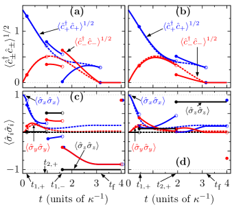
Figure 5: (Color online) Trajectories with imperfect detection ($\eta=0.9$ for both detectors), which leads to imperfect reversal of the measurement-induced dephasing. See Fig. 4 for the values of other simulation parameters and an explanation of the symbols.

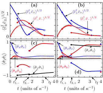
Figure 6: (Color online) Trajectories in the presence of qubit relaxation at a rate $0.1\times\kappa/\pi$. See Fig. 4 for the values of other simulation parameters and an explanation of the symbols.

Here we briefly discuss the effect of imperfect photodetection and of qubit relaxation. We point out some issues that inevitably arise in experimental realizations but do not attempt to thoroughly map the effects of non-idealities. We do this by presenting numerical solutions to Eq. (9).

Figure 5 presents example trajectories for imperfect detection efficiency ($\eta=0.9$). The possibility of missing photons leads to a mixed state and prevents fully reversing the measurement-induced dephasing, i.e., $\left\langle\hat{\sigma}_{x,1}\hat{\sigma}_{x,2}\right\rangle<1$ at $t=t_{\textrm{f}}$. However, the unconditioned master equation [Eq. (16)] is unchanged and the parity of the initial state is correctly measured, as long as sufficiently many photons are detected.

Figure 6 shows trajectories for a non-zero qubit relaxation rate. Specifically, we add $\mathcal{D}\left[\sqrt{\mbox{$\gamma$}}\hat{\sigma}_{-,j}\right]\hat{\rho}_{I}$ for each qubit $j$ to the right-hand side of Eq. (9). We choose $\gamma=0.1\times\kappa/\pi$. As in the case of inefficient detection, the qubit relaxation prevents perfect reversal of the measurement-induced dephasing. In addition, qubit decay leads to a mixed resonator state even at $t_{\textrm{f}}$. This implies that the displacements in step 4 of the protocol cannot restore the resonators to vacuum perfectly, i.e., $\langle\hat{c}_{\pm}^{\dagger}\hat{c}_{\pm}\rangle>0$ even after $t=t_{\textrm{f}}$. Visually the most striking phenomenon in Fig. 6 is the non-conservation of parity but it occurs even without performing the measurement, i.e., even if we were to choose $\alpha=0$.

References

- Cirac and Zoller (1995) J. I. Cirac and P. Zoller, Phys. Rev. Lett. 74, 4091 (1995).
- Cabrillo et al. (1999) C. Cabrillo, J. I. Cirac, P. García-Fernández, and P. Zoller, Phys. Rev. A 59, 1025 (1999).
- Bose et al. (1999) S. Bose, P. L. Knight, M. B. Plenio, and V. Vedral, Phys. Rev. Lett. 83, 5158 (1999).
- Duan and Kimble (2003) L. M. Duan and H. J. Kimble, Phys. Rev. Lett. 90, 253601 (2003).
- Browne et al. (2003) D. E. Browne, M. B. Plenio, and S. F. Huelga, Phys. Rev. Lett. 91, 067901 (2003).
- Barrett and Kok (2005) S. D. Barrett and P. Kok, Phys. Rev. A 71, 060310 (2005).
- Lim et al. (2005) Y. L. Lim, A. Beige, and L. C. Kwek, Phys. Rev. Lett. 95, 030505 (2005).
- Ladd et al. (2006) T. D. Ladd, P. van Loock, K. Nemoto, W. J. Munro, and Y. Yamamoto, New J. Phys. 8, 184 (2006).
- Busch et al. (2008) J. Busch, E. S. Kyoseva, M. Trupke, and A. Beige, Phys. Rev. A 78, 040301 (2008).
- Matsuzaki et al. (2011) Y. Matsuzaki, S. C. Benjamin, and J. Fitzsimons, Phys. Rev. A 83, 060303 (2011).
- Azuma et al. (2012) K. Azuma, H. Takeda, M. Koashi, and N. Imoto, Phys. Rev. A 85, 062309 (2012).
- Bernien et al. (2013) H. Bernien, B. Hensen, W. Pfaff, G. Koolstra, M. S. Blok, L. Robledo, T. H. Taminiau, M. Markham, D. J. Twitchen, L. Childress, and R. Hanson, Nature (London) 497, 86 (2013).
- Bruschi et al. (2014) D. E. Bruschi, T. M. Barlow, M. Razavi, and A. Beige, Phys. Rev. A 90, 032306 (2014).
- Briegel et al. (1998) H. J. Briegel, W. Dür, J. I. Cirac, and P. Zoller, Phys. Rev. Lett. 81, 5932 (1998).
- Kok et al. (2007) P. Kok, K. Nemoto, T. C. Ralph, J. P. Dowling, and G. J. Milburn, Rev. Mod. Phys. 79, 135 (2007).
- Terhal (2015) B. M. Terhal, Rev. Mod. Phys. 87, 307 (2015).
- Bravyi et al. (2010) S. Bravyi, D. Poulin, and B. Terhal, Phys. Rev. Lett. 104, 050503 (2010).
- Blais et al. (2004) A. Blais, R.-S. Huang, A. Wallraff, S. M. Girvin, and R. J. Schoelkopf, Phys. Rev. A 69, 062320 (2004).
- Wallraff et al. (2004) A. Wallraff, D. I. Schuster, A. Blais, L. Frunzio, R.-S. Huang, J. Majer, S. Kumar, S. M. Girvin, and R. J. Schoelkopf, Nature (London) 431, 162 (2004).
- Devoret and Schoelkopf (2013) M. H. Devoret and R. J. Schoelkopf, Science 339, 1169 (2013).
- Kelly et al. (2015) J. Kelly, R. Barends, A. G. Fowler, A. Megrant, E. Jeffrey, T. C. White, D. Sank, J. Y. Mutus, B. Campbell, Y. Chen, Z. Chen, B. Chiaro, A. Dunsworth, I. C. Hoi, C. Neill, P. J. J. O’Malley, C. Quintana, P. Roushan, A. Vainsencher, J. Wenner, A. N. Cleland, and J. M. Martinis, Nature (London) 519, 66 (2015).
- Romero et al. (2009) G. Romero, J. J. García-Ripoll, and E. Solano, Phys. Rev. Lett. 102, 173602 (2009).
- Chen et al. (2011) Y. F. Chen, D. Hover, S. Sendelbach, L. Maurer, S. T. Merkel, E. J. Pritchett, F. K. Wilhelm, and R. McDermott, Phys. Rev. Lett. 107, 217401 (2011).
- Peropadre et al. (2011) B. Peropadre, G. Romero, G. Johansson, C. M. Wilson, E. Solano, and J. J. García-Ripoll, Phys. Rev. A 84, 063834 (2011).
- Fan et al. (2013) B. Fan, A. F. Kockum, J. Combes, G. Johansson, I.-C. Hoi, C. M. Wilson, P. Delsing, G. J. Milburn, and T. M. Stace, Phys. Rev. Lett. 110, 053601 (2013).
- Hoi et al. (2013) I.-C. Hoi, A. F. Kockum, T. Palomaki, T. M. Stace, B. Fan, L. Tornberg, S. R. Sathyamoorthy, G. Johansson, P. Delsing, and C. M. Wilson, Phys. Rev. Lett. 111, 053601 (2013).
- Sathyamoorthy et al. (2014) S. R. Sathyamoorthy, L. Tornberg, A. F. Kockum, B. Q. Baragiola, J. Combes, C. M. Wilson, T. M. Stace, and G. Johansson, Phys. Rev. Lett. 112, 093601 (2014).
- Fan et al. (2014) B. Fan, G. Johansson, J. Combes, G. J. Milburn, and T. M. Stace, Phys. Rev. B 90, 035132 (2014).
- Govenius et al. (2014) J. Govenius, R. E. Lake, K. Y. Tan, V. Pietilä, J. K. Julin, I. J. Maasilta, P. Virtanen, and M. Möttönen, Phys. Rev. B 90, 064505 (2014).
- Gasparinetti et al. (2015) S. Gasparinetti, K. L. Viisanen, O.-P. Saira, T. Faivre, M. Arzeo, M. Meschke, and J. P. Pekola, Phys. Rev. Appl. 3, 014007 (2015).
- Koshino et al. (2015) K. Koshino, K. Inomata, Z. Lin, Y. Nakamura, and T. Yamamoto, Phys. Rev. A 91, 043805 (2015).
- Schuster et al. (2007) D. I. Schuster, A. A. Houck, J. A. Schreier, A. Wallraff, J. M. Gambetta, A. Blais, L. Frunzio, J. Majer, B. Johnson, M. H. Devoret, S. M. Girvin, and R. J. Schoelkopf, Nature (London) 445, 515 (2007).
- Kerckhoff et al. (2009) J. Kerckhoff, L. Bouten, A. Silberfarb, and H. Mabuchi, Phys. Rev. A 79, 024305 (2009).
- Roch et al. (2014) N. Roch, M. E. Schwartz, F. Motzoi, C. Macklin, R. Vijay, A. W. Eddins, A. N. Korotkov, K. B. Whaley, M. Sarovar, and I. Siddiqi, Phys. Rev. Lett. 112, 170501 (2014).
- Schuster et al. (2005) D. I. Schuster, A. Wallraff, A. Blais, L. Frunzio, R.-S. Huang, J. Majer, S. M. Girvin, and R. J. Schoelkopf, Phys. Rev. Lett. 94, 123602 (2005).
- Gambetta et al. (2006) J. Gambetta, A. Blais, D. I. Schuster, A. Wallraff, L. Frunzio, J. Majer, M. H. Devoret, S. M. Girvin, and R. J. Schoelkopf, Phys. Rev. A 74, 042318 (2006).
- Gambetta et al. (2008) J. Gambetta, A. Blais, M. Boissonneault, A. A. Houck, D. I. Schuster, and S. M. Girvin, Phys. Rev. A 77, 012112 (2008).
- Lalumière et al. (2010) K. Lalumière, J. M. Gambetta, and A. Blais, Phys. Rev. A 81, 040301 (2010).
- Tornberg and Johansson (2010) L. Tornberg and G. Johansson, Phys. Rev. A 82, 012329 (2010).
- Riste et al. (2013) D. Riste, M. Dukalski, C. A. Watson, G. de Lange, M. J. Tiggelman, Y. Blanter, K. W. Lehnert, R. N. Schouten, and L. DiCarlo, Nature (London) 502, 350 (2013).
- Korotkov and Jordan (2006) A. N. Korotkov and A. N. Jordan, Phys. Rev. Lett. 97, 166805 (2006).
- Frisk Kockum et al. (2012) A. Frisk Kockum, L. Tornberg, and G. Johansson, Phys. Rev. A 85, 052318 (2012).
- de Lange et al. (2014) G. de Lange, D. Ristè, M. J. Tiggelman, C. Eichler, L. Tornberg, G. Johansson, A. Wallraff, R. N. Schouten, and L. DiCarlo, Phys. Rev. Lett. 112, 080501 (2014).
- Clerk et al. (2010) A. A. Clerk, M. H. Devoret, S. M. Girvin, F. Marquardt, and R. J. Schoelkopf, Rev. Mod. Phys. 82, 1155 (2010).
- Wiseman and Milburn (2010) H. M. Wiseman and G. J. Milburn, Quantum measurement and control (Cambridge University Press, 2010).
- Hutchison et al. (2009) C. L. Hutchison, J. M. Gambetta, A. Blais, and F. K. Wilhelm, Can. J. Phys. 87, 225 (2009).
- Bishop et al. (2009) L. S. Bishop, L. Tornberg, D. Price, E. Ginossar, A. Nunnenkamp, A. A. Houck, J. M. Gambetta, J. Koch, G. Johansson, S. M. Girvin, and R. J. Schoelkopf, New J. Phys. 11, 073040 (2009).
- Helmer and Marquardt (2009) F. Helmer and F. Marquardt, Phys. Rev. A 79, 052328 (2009).
- Nigg and Girvin (2013) S. E. Nigg and S. M. Girvin, Phys. Rev. Lett. 110, 243604 (2013).
- Govia et al. (2015) L. C. G. Govia, E. J. Pritchett, B. L. T. Plourde, M. G. Vavilov, R. McDermott, and F. K. Wilhelm, Phys. Rev. A 92, 022335 (2015).
- Viola et al. (1999) L. Viola, E. Knill, and S. Lloyd, Phys. Rev. Lett. 82, 2417 (1999).
- Paik et al. (2011) H. Paik, D. I. Schuster, L. S. Bishop, G. Kirchmair, G. Catelani, A. P. Sears, B. R. Johnson, M. J. Reagor, L. Frunzio, L. I. Glazman, S. M. Girvin, M. H. Devoret, and R. J. Schoelkopf, Phys. Rev. Lett. 107, 240501 (2011).
- Rigetti et al. (2012) C. Rigetti, J. M. Gambetta, S. Poletto, B. L. T. Plourde, J. M. Chow, A. D. Córcoles, J. A. Smolin, S. T. Merkel, J. R. Rozen, G. A. Keefe, M. B. Rothwell, M. B. Ketchen, and M. Steffen, Phys. Rev. B 86, 100506 (2012).
- Barends et al. (2013) R. Barends, J. Kelly, A. Megrant, D. Sank, E. Jeffrey, Y. Chen, Y. Yin, B. Chiaro, J. Mutus, C. Neill, P. O’Malley, P. Roushan, J. Wenner, T. C. White, A. N. Cleland, and J. M. Martinis, Phys. Rev. Lett. 111, 080502 (2013).
- Göppl et al. (2008) M. Göppl, A. Fragner, M. Baur, R. Bianchetti, S. Filipp, J. M. Fink, P. J. Leek, G. Puebla, L. Steffen, and A. Wallraff, J. Appl. Phys. 104, 113904 (2008).
- Osborn et al. (2007) K. D. Osborn, J. A. Strong, A. J. Sirois, and R. W. Simmonds, IEEE Trans. Appl. Supercond. 17, 166 (2007).
- Pierre et al. (2014) M. Pierre, I.-M. Svensson, S. R. Sathyamoorthy, G. Johansson, and P. Delsing, Appl. Phys. Lett. 104, 232604 (2014).