Learning with Symmetric Label Noise: The Importance of Being Unhinged

Abstract

Convex potential minimisation is the de facto approach to binary classification. However, Long and Servedio (2010) proved that under symmetric label noise (SLN), minimisation of any convex potential over a linear function class can result in classification performance equivalent to random guessing. This ostensibly shows that convex losses are not SLN-robust. In this paper, we propose a convex, classification-calibrated loss and prove that it is SLN-robust. The loss avoids the Long and Servedio (2010) result by virtue of being negatively unbounded. The loss is a modification of the hinge loss, where one does not clamp at zero; hence, we call it the unhinged loss. We show that the optimal unhinged solution is equivalent to that of a strongly regularised SVM, and is the limiting solution for any convex potential; this implies that strong $\ell_{2}$ regularisation makes most standard learners SLN-robust. Experiments confirm the SLN-robustness of the unhinged loss.

1 Learning with symmetric label noise

Binary classification is the canonical supervised learning problem. Given an instance space $\mathscr{X}$, and samples from some distribution $D$ over $\mathscr{X}\times\{\pm 1\}$, the goal is to learn a scorer $s\colon\mathscr{X}\to\mathbb{R}$ with low misclassification error on future samples drawn from $D$. Our interest is in the more realistic scenario where the learner observes samples from a distribution $\accentset{\rule{2.79996pt}{0.6pt}}{D}$, which is a corruption of $D$ where labels have some constant probability of being flipped. The goal is still to perform well with respect to the unobserved distribution $D$. This is known as the problem of learning from symmetric label noise (SLN learning) (Angluin and Laird, 1988).

Long and Servedio (2010) proved the following negative result on what is possible in SLN learning: there exists a linearly separable $D$ where, when the learner observes some corruption $\accentset{\rule{2.79996pt}{0.6pt}}{D}$ with symmetric label noise of any nonzero rate, minimisation of any convex potential over a linear function class results in classification performance on $D$ that is equivalent to random guessing. Ostensibly, this establishes that convex losses are not “SLN-robust” and motivates the use of non-convex losses (Stempfel and Ralaivola, 2009; Masnadi-Shirazi et al., 2010; Ding and Vishwanathan, 2010; Denchev et al., 2012; Manwani and Sastry, 2013).

In this paper, we propose a convex loss and prove that it is SLN-robust. The loss avoids the result of Long and Servedio (2010) by virtue of being negatively unbounded. The loss is a modification of the hinge loss where one does not clamp at zero; thus, we call it the unhinged loss. We show that this is the unique convex loss (up to scaling and translation) that satisfies a notion of “strong SLN-robustness ” (Proposition 4). In addition to being SLN-robust, this loss has several attractive properties, such as being classification-calibrated (Proposition 5), consistent when minimised on the corrupted distribution (Proposition 6), and having an easily computable optimal solution that is the difference of two kernel means (Equation 9). Finally, we show that this optimal solution is equivalent to that of a strongly regularised SVM (Proposition 7), and such a result holds more generally for any twice-differentiable convex potential (Proposition 8), implying that strong $\ell_{2}$ regularisation endows most standard learners with SLN-robustness.

The classifier resulting from minimising the unhinged loss is not new (Devroye et al., 1996, Chapter 10), (Schölkopf and Smola, 2002, Section 1.2), (Shawe-Taylor and Cristianini, 2004, Section 5.1). However, establishing this classifier’s SLN-robustness, its equivalence to a highly regularised SVM solution, and showing the underlying loss uniquely satisfies a notion of strong SLN-robustness, to our knowledge is novel.

2 Background and problem setup

Fix an instance space $\mathscr{X}$. We denote by $D$ some distribution over $\mathscr{X}\times\{\pm 1\}$, with random variables $(\mathsf{X},\mathsf{Y})\sim D$. Any $D$ may be expressed via the class-conditional distributions $(P,Q)=(\mathbb{P}(\mathsf{X}\mid\mathsf{Y}=1),\mathbb{P}(\mathsf{X}\mid\mathsf{Y}=-1))$ and base rate $\pi=\mathbb{P}(\mathsf{Y}=1)$, or equivalently via the marginal distribution $M=\mathbb{P}(\mathsf{X})$ and class-probability function $\eta\colon x\mapsto\mathbb{P}(\mathsf{Y}=1\mid\mathsf{X}=x)$. We interchangeably write $D$ as $D_{P,Q,\pi}$ or $D_{M,\eta}$.

2.1 Classifiers, scorers, and risks

A scorer is any function $s\colon\mathscr{X}\to\mathbb{R}$. A loss is any function $\ell\colon\{\pm 1\}\times\mathbb{R}\to\mathbb{R}$. We use $\ell_{-1},\ell_{1}$ to refer to $\ell(-1,\cdot)$ and $\ell(1,\cdot)$. The $\ell$-conditional risk $L_{\ell}\colon[0,1]\times\mathbb{R}\to\mathbb{R}$ is defined as $L_{\ell}\colon(\eta,v)\mapsto\eta\cdot\ell_{1}(v)+(1-\eta)\cdot\ell_{-1}(v).$ Given a distribution $D$, the $\ell$-risk of a scorer $s$ is defined as

$$\mathbb{L}^{D}_{\ell}(s) \stackrel{{\scriptstyle.}}{{=}}\underset{(\mathsf{X},\mathsf{Y})\sim D}{\mathbb{E}}\left[\ell(\mathsf{Y},s(\mathsf{X}))\right],$$ (1)

or equivalently $\mathbb{L}^{D}_{\ell}(s)=\underset{\mathsf{X}\sim M}{\mathbb{E}}\left[L_{\ell}(\eta(\mathsf{X}),s(\mathsf{X}))\right]$. For a set $\mathscr{S}$, $\mathbb{L}^{D}_{\ell}(\mathscr{S})$ is the set of $\ell$-risks for all scorers in $\mathscr{S}$.

A function class is any $\mathscr{F}\subseteq\mathbb{R}^{\mathscr{X}}$. Given some $\mathscr{F}$, the set of restricted Bayes-optimal scorers for a loss $\ell$ are those scorers in $\mathscr{F}$ that minimise the $\ell$-risk:

$$\mathscr{S}^{D,\mathscr{F},*}_{\ell}\stackrel{{\scriptstyle.}}{{=}}\underset{s\in\mathscr{F}}{\operatorname{Argmin}}\,\mathbb{L}^{D}_{\ell}(s).$$

The set of (unrestricted) Bayes-optimal scorers is $\mathscr{S}^{D,*}_{\ell}=\mathscr{S}^{D,\mathscr{F},*}_{\ell}$ for $\mathscr{F}=\mathbb{R}^{\mathscr{X}}$. The restricted $\ell$-regret of a scorer is its excess risk over that of any restricted Bayes-optimal scorer:

$$\mathrm{regret}^{D,\mathscr{F}}_{\ell}(s)\stackrel{{\scriptstyle.}}{{=}}\mathbb{L}^{D}_{\ell}(s)-\inf_{t\in\mathscr{F}}\mathbb{L}^{D}_{\ell}(t).$$

Binary classification is concerned with the risk corresponding to the zero-one loss, $\ell^{01}\colon(y,v)\mapsto\llbracket yv<0\rrbracket+\frac{1}{2}\llbracket v=0\rrbracket$. A loss $\ell$ is classification-calibrated if all its Bayes-optimal scorers are also optimal for zero-one loss: $(\forall D)\,\mathscr{S}^{D,*}_{\ell}\subseteq\mathscr{S}^{D,*}_{01}.$ A convex potential is any loss $\ell\colon(y,v)\mapsto\phi(yv)$, where $\phi\colon\mathbb{R}\to\mathbb{R}_{+}$ is convex, non-increasing, differentiable with $\phi^{\prime}(0)<0$, and $\phi(+\infty)=0$ (Long and Servedio, 2010, Definition 1). All convex potential losses are classification-calibrated (Bartlett et al., 2006, Theorem 2.1).

2.2 Learning with symmetric label noise (SLN learning)

The problem of learning with symmetric label noise (SLN learning) is the following (Angluin and Laird, 1988; Kearns, 1998; Blum and Mitchell, 1998; Natarajan et al., 2013). For some notional “clean” distribution $D$, which we would like to observe, we instead observe samples from some corrupted distribution $\mathrm{SLN}(D,\rho)$, for some $\rho\in[0,{1}/{2})$. The distribution $\mathrm{SLN}(D,\rho)$ is such that the marginal distribution of instances is unchanged, but each label is independently flipped with probability $\rho$. The goal is to learn a scorer from these corrupted samples such that $\mathbb{L}^{D}_{01}(s)$ is small.

For any quantity in $D$, we denote its corrupted counterparts in $\mathrm{SLN}(D,\rho)$ with a bar, e.g. $\accentset{\rule{2.79996pt}{0.6pt}}{M}$ for the corrupted marginal distribution, and $\accentset{\rule{2.79996pt}{0.6pt}}{\eta}$ for the corrupted class-probability function; additionally, when $\rho$ is clear from context, we will occasionally refer to $\mathrm{SLN}(D,\rho)$ by $\accentset{\rule{2.79996pt}{0.6pt}}{D}$. By definition of the corruption process, the corruption marginal distribution $\accentset{\rule{2.79996pt}{0.6pt}}{M}=M$, and (Natarajan et al., 2013, Lemma 7)

$$(\forall x\in\mathscr{X})\,\accentset{\rule{2.79996pt}{0.6pt}}{\eta}(x)=(1-2\rho)\cdot\eta(x)+\rho.$$ (2)

3 SLN-robustness: formalisation

For our purposes, a learner $(\ell,\mathscr{F})$ comprises a loss $\ell$, and a function class $\mathscr{F}$, with learning being the search for some $s\in\mathscr{F}$ that minimises the $\ell$-risk. Informally, the learner $(\ell,\mathscr{F})$ is “robust” to symmetric label noise (SLN-robust) if minimising $\ell$ over $\mathscr{F}$ gives the same classifier on both the clean distribution $D$, which the learner would like to observe, and $\mathrm{SLN}(D,\rho)$ for any $\rho\in[0,1/2)$, which the learner actually observes. We now formalise this notion, and review what is known about the existence of SLN-robust learners.

3.1 SLN-robust learners: a formal definition

For some fixed instance space $\mathscr{X}$, let $\Delta$ denote the set of distributions on $\mathscr{X}\times\{\pm 1\}$. Given a notional “clean” distribution $D$, $\mathcal{N}_{\mathrm{sln}}\colon\Delta\to 2^{\Delta}$ returns the set of possible corrupted versions of $D$ the learner may observe, where labels are flipped with unknown probability $\rho$:

$$\mathcal{N}_{\mathrm{sln}}\colon D\mapsto\left\{\mathrm{SLN}(D,\rho)\mid\rho\in\left[0,\frac{1}{2}\right)\right\}.$$

Equipped with this, we define our notion of SLN-robustness.

Definition 1 (SLN-robustness).

We say that a learner $(\ell,\mathscr{F})$ is SLN-robust if

$$(\forall D\in\Delta)\,(\forall\accentset{\rule{2.79996pt}{0.6pt}}{D}\in\mathcal{N}_{\mathrm{sln}}(D))\,\mathbb{L}^{D}_{01}(\mathscr{S}^{D,\mathscr{F},*}_{\ell})=\mathbb{L}^{D}_{01}(\mathscr{S}^{\accentset{\rule{2.79996pt}{0.6pt}}{D},\mathscr{F},*}_{\ell}).$$ (3)

That is, SLN-robustness requires that for any level of label noise in the observed distribution $\accentset{\rule{2.79996pt}{0.6pt}}{D}$, the classification performance (wrt $D$) of the learner is the same as if the learner directly observes $D$. Unfortunately, as we will now see, a widely adopted class of learners is not SLN-robust.

3.2 Convex potentials with linear function classes are not SLN-robust

Fix $\mathscr{X}=\mathbb{R}^{d}$, and consider learners employing a convex potential $\ell$, and a function class of linear scorers

$$\mathscr{F}_{\mathrm{lin}}=\{x\mapsto\langle w,x\rangle\mid w\in\mathbb{R}^{d}\}.$$

This captures e.g. the linear SVM and logistic regression, which are widely studied in theory and applied in practice. Unfortunately, these learners are not SLN-robust: Long and Servedio (2010, Theorem 2) give an example where, when learning under symmetric label noise, for any convex potential $\ell$, the corrupted $\ell$-risk minimiser over $\mathscr{F}_{\mathrm{lin}}$ has classification performance equivalent to random guessing on $D$. This implies that $(\ell,\mathscr{F}_{\mathrm{lin}})$ is not SLN-robust as per Definition 1. (All Proofs may be found in Appendix A.)

Proposition 1 (Long and Servedio (2010, Theorem 2)).

Let $\mathscr{X}=\mathbb{R}^{d}$ for any $d\geq 2$. Pick any convex potential $\ell$. Then, $(\ell,\mathscr{F}_{\mathrm{lin}})$ is not SLN-robust.

The widespread practical use of convex potential based learners makes Proposition 1 a disheartening result, and motivates the search for other learners that are SLN-robust.

3.3 The fallout: what learners are SLN-robust?

In light of Proposition 1, there are two ways to proceed in order to obtain SLN-robust learners: either we change the class of losses $\ell$, or we change the function class $\mathscr{F}$.

The first approach has been pursued in a large body of work that embraces non-convex losses (Stempfel and Ralaivola, 2009; Masnadi-Shirazi et al., 2010; Ding and Vishwanathan, 2010; Denchev et al., 2012; Manwani and Sastry, 2013). However, while such losses avoid the conditions of Proposition 1, this does not automatically imply that they are SLN-robust when used with $\mathscr{F}_{\mathrm{lin}}$. In Appendix B, we present evidence that some of these losses are in fact not SLN-robust when used with $\mathscr{F}_{\mathrm{lin}}$.

The second approach is to instead consider suitably rich $\mathscr{F}$ that contains the Bayes-optimal scorer for $\accentset{\rule{2.79996pt}{0.6pt}}{D}$, e.g. by employing a universal kernel. With this choice, one can still use a convex potential loss; in fact, owing to Equation 2, using any classification-calibrated loss will result in an SLN-robust learner when $\mathscr{F}=\mathbb{R}^{\mathscr{X}}$.

Proposition 2.

Pick any classification-calibrated $\ell$. Then, $(\ell,\mathbb{R}^{\mathscr{X}})$ is SLN-robust.

Both approaches have drawbacks. The first approach has a computational penalty, as it requires optimising a non-convex loss. The second approach has a statistical penalty, as estimation rates with a rich $\mathscr{F}$ will require a larger sample size. Thus, it appears that SLN-robustness involves a computational-statistical tradeoff.

However, there is a variant of the first option: pick a loss that is convex, but not a convex potential. If an SLN-robust loss of this type exists, it affords the computational and statistical advantages of minimising convex risks with linear scorers. Manwani and Sastry (2013) demonstrated that square loss, $\ell(y,v)=(1-yv)^{2}$, is one such loss. We will show that there is a simpler loss that is similarly convex, classification-calibrated, and SLN-robust, but is not in the class of convex potentials by virtue of being negatively unbounded. To derive this loss, it is helpful to interpret robustness in terms of a noise-correction procedure on loss functions.

4 SLN-robustness: a noise-corrected loss perspective

The definition of SLN-robustness (Equation 3) involves optimal scorers with the same loss $\ell$ over two different distributions. We now re-express this to reason about optimal scorers on the same distribution, but with two different losses. This will help characterise the set of losses that are SLN-robust.

4.1 Reformulating SLN-robustness via noise-corrected losses

Given any $\rho\in[0,1/2)$, Natarajan et al. (2013, Lemma 1) showed how to associate with a loss $\ell$ a noise-corrected counterpart $\accentset{\rule{2.79996pt}{0.6pt}}{\ell}$, such that for any $D$, $\mathbb{L}^{D}_{\ell}(s)=\mathbb{L}^{\accentset{\rule{2.79996pt}{0.6pt}}{D}}_{\accentset{\rule{2.79996pt}{0.6pt}}{\ell}}(s)$. The loss $\accentset{\rule{2.79996pt}{0.6pt}}{\ell}$ is defined as follows.

Definition 2 (Noise-corrected loss).

Given any loss $\ell$ and $\rho\in[0,1/2)$, the noise-corrected loss $\accentset{\rule{2.79996pt}{0.6pt}}{\ell}$ is

$$(\forall y\in\{\pm 1\})\,(\forall v\in\mathbb{R})\,\accentset{\rule{2.79996pt}{0.6pt}}{\ell}(y,v)=\frac{{(1-\rho)}\cdot\ell(y,v)-{\rho}\cdot\ell(-y,v)}{1-2\rho}.$$ (4)

Since $\accentset{\rule{2.79996pt}{0.6pt}}{\ell}$ depends on the unknown parameter $\rho$, it is not directly usable to design an SLN-robust learner. Nonetheless, it is a useful theoretical construct, since the risk equivalence between $\mathbb{L}^{D}_{\ell}(s)$ and $\mathbb{L}^{\accentset{\rule{2.79996pt}{0.6pt}}{D}}_{\accentset{\rule{2.79996pt}{0.6pt}}{\ell}}(s)$ means that for any $\mathscr{F}$, minimisation of the $\ell$-risk on $D$ over $\mathscr{F}$ is equivalent to minimisation of the $\accentset{\rule{2.79996pt}{0.6pt}}{\ell}$-risk on $\accentset{\rule{2.79996pt}{0.6pt}}{D}$ over $\mathscr{F}$, i.e. $\mathscr{S}^{D,\mathscr{F},*}_{\ell}=\mathscr{S}^{\accentset{\rule{2.79996pt}{0.6pt}}{D},\mathscr{F},*}_{\accentset{\rule{2.79996pt}{0.6pt}}{\ell}}.$ With this, we can re-express the SLN-robustness of a learner $(\ell,\mathscr{F})$ as

$$(\forall D\in\Delta)\,(\forall\accentset{\rule{2.79996pt}{0.6pt}}{D}\in\mathcal{N}_{\mathrm{sln}}(D))\,\mathbb{L}^{D}_{01}(\mathscr{S}^{\accentset{\rule{2.79996pt}{0.6pt}}{D},\mathscr{F},*}_{\accentset{\rule{2.79996pt}{0.6pt}}{\ell}})=\mathbb{L}^{D}_{01}(\mathscr{S}^{\accentset{\rule{2.79996pt}{0.6pt}}{D},\mathscr{F},*}_{\ell}).$$ (5)

This reformulation is useful, because to characterise SLN-robustness of $(\ell,\mathscr{F})$, we can now consider conditions on $\ell$ such that $\ell$ and its noise-corrected counterpart $\accentset{\rule{2.79996pt}{0.6pt}}{\ell}$ induce the same restricted Bayes-optimal scorers.

4.2 Characterising a stronger notion of SLN-robustness

Manwani and Sastry (2013, Theorem 1) proved a sufficient condition on $\ell$ such that Equation 5 holds, namely,

$$(\exists C\in\mathbb{R})(\forall v\in\mathbb{R})\,\ell_{1}(v)+\ell_{-1}(v)=C.$$ (6)

For such a loss, $\accentset{\rule{2.79996pt}{0.6pt}}{\ell}$ is a scaled and translated version of $\ell$, so that trivially $\mathscr{S}^{\accentset{\rule{2.79996pt}{0.6pt}}{D},\mathscr{F},*}_{\ell}=\mathscr{S}^{\accentset{\rule{2.79996pt}{0.6pt}}{D},\mathscr{F},*}_{\accentset{\rule{2.79996pt}{0.6pt}}{\ell}}$.

Ideally, one would like to characterise when Equation 5 holds. While this is an open question, interestingly, we can show that under a stronger requirement on the losses $\ell$ and $\accentset{\rule{2.79996pt}{0.6pt}}{\ell}$, the condition in Equation 6 is also necessary. The stronger requirement is that the corresponding risks order all stochastic scorers identically. A stochastic scorer is simply a mapping $f\colon\mathscr{X}\to\Delta_{\mathbb{R}}$, where $\Delta_{\mathbb{R}}$ is the set of distributions over the reals. In a slight abuse of notation, we denote the $\ell$-stochastic risk of $f$ by

$$\mathbb{L}^{D}_{\ell}(f)=\underset{(\mathsf{X},\mathsf{Y})\sim D}{\mathbb{E}}\left[\underset{\mathsf{S}\sim f(\mathsf{X})}{\mathbb{E}}\left[\ell(\mathsf{Y},\mathsf{S})\right]\right].$$

Equipped with this, we define a notion of order equivalence of loss pairs.

Definition 3 (Order equivalent loss pairs).

We say that a pair of losses $(\ell,\tilde{\ell})$ are order equivalent if

$$(\forall D)\,(\forall f,g\in\Delta_{\mathbb{R}}^{\mathscr{X}})\,\mathbb{L}^{D}_{\ell}(f)\leq\mathbb{L}^{D}_{\ell}(g)\iff\mathbb{L}^{D}_{\tilde{\ell}}(f)\leq\mathbb{L}^{D}_{\tilde{\ell}}(g).$$

Clearly, if two losses are order equivalent, their corresponding risks have the same restricted minimisers. Consequently, if $(\ell,\accentset{\rule{2.79996pt}{0.6pt}}{\ell})$ are order equivalent for every $\rho\in[0,1/2)$, this implies that $\mathscr{S}^{\accentset{\rule{2.79996pt}{0.6pt}}{D},\mathscr{F},*}_{\ell}=\mathscr{S}^{\accentset{\rule{2.79996pt}{0.6pt}}{D},\mathscr{F},*}_{\accentset{\rule{2.79996pt}{0.6pt}}{\ell}}$ for any $\mathscr{F}$, which by Equation 5 means that for any $\mathscr{F}$, the learner $(\ell,\mathscr{F})$ is SLN-robust. We can thus think of order equivalence of $(\ell,\accentset{\rule{2.79996pt}{0.6pt}}{\ell})$ as signifying strong SLN-robustness of a loss $\ell$.

Definition 4 (Strong SLN-robustness).

We say a loss $\ell$ is strongly SLN-robust if for every $\rho\in[0,1/2)$, $(\ell,\accentset{\rule{2.79996pt}{0.6pt}}{\ell})$ are order equivalent.

We establish that the sufficient condition of Equation 6 is also necessary for strong SLN-robustness of $\ell$.

Proposition 3.

A loss $\ell$ is strongly SLN-robust if and only if it satisfies Equation 6.

We now return to our original goal, which was to find a convex $\ell$ that is SLN-robust for $\mathscr{F}_{\mathrm{lin}}$ (and ideally more general function classes). The above suggests that to do so, it is reasonable to consider as admissible those losses that satisfy Equation 6. Unfortunately, it is evident that if $\ell$ is convex, non-constant, and bounded below by zero, then it cannot possibly be admissible in this sense. But we now show that removing the boundedness restriction allows for the existence of a convex admissible loss.

5 The unhinged loss: a convex, classification-calibrated, strongly SLN-robust loss

Consider the following simple, but non-standard convex loss:

$$\ell^{\mathrm{unh}}_{1}(v) =1-v\text{ and }\ell^{\mathrm{unh}}_{-1}(v)=1+v.$$

A peculiar property of the loss is that it is negatively unbounded, an issue we discuss in §5.3. Compared to the hinge loss, the loss does not clamp at zero, i.e. it does not have a hinge. Thus, we call this the unhinged loss. The loss has a number of attractive properties, the most immediate of which is its SLN-robustness.

5.1 The unhinged loss is strongly SLN-robust

Since $\ell^{\mathrm{unh}}_{1}(v)+\ell^{\mathrm{unh}}_{-1}(v)=0$ we conclude from Proposition 3 that $\ell^{\mathrm{unh}}$ is strongly SLN-robust, and thus that $(\ell^{\mathrm{unh}},\mathscr{F})$ is SLN-robust for any choice of $\mathscr{F}$. Further, the following uniqueness property is not hard to show.

Proposition 4.

Pick any convex loss $\ell$. Then,

$$(\exists C\in\mathbb{R})\,\ell_{1}(v)+\ell_{-1}(v)=C\iff(\exists A,B,D\in\mathbb{R})\,\ell_{1}(v)=-A\cdot v+B,\ell_{-1}(v)=A\cdot v+D.$$

That is, up to scaling and translation, $\ell^{\mathrm{unh}}$ is the only convex loss that is strongly SLN-robust.

Returning to the case of linear scorers, the above implies that $(\ell^{\mathrm{unh}},\mathscr{F}_{\mathrm{lin}})$ is SLN-robust. This does not contradict Proposition 1, since $\ell^{\mathrm{unh}}$ is not a convex potential as it is negatively unbounded. Intuitively, this property allows the loss to compensate for the high penalty incurred by instances that are misclassified with high margin by allowing for a high gain for instances that correctly classified with high margin.

5.2 The unhinged loss is classification calibrated

SLN-robustness is by itself insufficient for a learner to be useful. For example, a loss that is uniformly zero is strongly SLN-robust, but is useless as it is not classification-calibrated. Fortunately, the unhinged loss is classification-calibrated, as we now establish. For reasons that shall be discussed subsequently, we consider minimisation of the risk over $\mathscr{F}_{B}=[-B,+B]^{\mathscr{X}}$, the set of scorers with range bounded by $B\in[0,\infty)$.

Proposition 5.

Fix $\ell=\ell^{\mathrm{unh}}$. Then, for any $D_{M,\eta}$, $B\in[0,\infty)$, $\mathscr{S}^{D,\mathscr{F}_{B},*}_{\ell}=\{x\mapsto B\cdot\operatorname{sign}(2\eta(x)-1)\}.$

Thus, for every $B\in[0,\infty)$, the restricted Bayes-optimal scorer over $\mathscr{F}_{B}$ has the same sign as the Bayes-optimal classifier for 0-1 loss. In the limiting case where $\mathscr{F}=\mathbb{R}^{\mathscr{X}}$, the optimal scorer is attainable if we operate over the extended reals $\mathbb{R}\cup\{\pm\infty\}$, in which case we can conclude that $\ell^{\mathrm{unh}}$ is classification-calibrated.

5.3 Enforcing boundedness of the loss

While the classification-calibration of $\ell^{\mathrm{unh}}$ is encouraging, Proposition 5 implies that its (unrestricted) Bayes-risk is $-\infty$. Thus, the regret of every non-optimal scorer $s$ is identically $+\infty$, which hampers analysis of consistency. In orthodox decision theory, analogous theoretical issues arise when attempting to establish basic theorems with unbounded losses (Ferguson, 1967, pg. 78), (Schervish, 1995, pg. 172).

We can side-step this issue by restricting attention to bounded scorers, so that $\ell^{\mathrm{unh}}$ is effectively bounded. By Proposition 5, this does not affect the classification-calibration of the loss. In the context of linear scorers, boundedness of scorers can be achieved by regularisation: instead of working with $\mathscr{F}_{\mathrm{lin}}$, one can instead use $\mathscr{F}_{\mathrm{lin},\lambda}=\{x\mapsto\langle w,x\rangle\mid||w||_{2}\leq 1/\sqrt{\lambda}\}$, where $\lambda>0$, so that $\mathscr{F}_{\mathrm{lin},\lambda}\subseteq\mathscr{F}_{R/\sqrt{\lambda}}$ for $R=\sup_{x\in\mathscr{X}}||x||_{2}$. Observe that restricting to bounded scorers does not affect the SLN-robustness of $\ell^{\mathrm{unh}}$, because $(\ell^{\mathrm{unh}},\mathscr{F})$ is SLN-robust for any $\mathscr{F}$. Thus, for example, $(\ell^{\mathrm{unh}},\mathscr{F}_{\mathrm{lin},\lambda})$ is SLN-robust for any $\lambda>0$. As we shall see in §6.3, working with $\mathscr{F}_{\mathrm{lin},\lambda}$ also lets us establish SLN-robustness of the hinge loss when $\lambda$ is large.

5.4 Unhinged loss minimisation on corrupted distribution is consistent

Using bounded scorers makes it possible to establish a surrogate regret bound for the unhinged loss. This shows classification consistency of unhinged loss minimisation on the corrupted distribution.

Proposition 6.

Fix $\ell=\ell^{\mathrm{unh}}$. Then, for any $D,\rho\in[0,1/2)$, $B\in[1,\infty)$, and scorer $s\in\mathscr{F}_{B}$,

$$\mathrm{regret}^{D}_{01}(s)\leq\mathrm{regret}^{D,\mathscr{F}_{B}}_{\ell}(s)=\frac{1}{1-2\rho}\cdot\mathrm{regret}^{\accentset{\rule{2.79996pt}{0.6pt}}{D},\mathscr{F}_{B}}_{\ell}(s).$$

Standard rates of convergence via generalisation bounds are also trivial to derive; see Appendix D. We now turn to the question of how to minimise the unhinged loss when using a kernelised scorer.

6 Learning with the unhinged loss and kernels

We now show that the optimal solution for the unhinged loss when employing regularisation and kernelised scorers has a simple form. This sheds further light on SLN-robustness and regularisation.

6.1 The centroid classifier optimises the unhinged loss

Consider minimising the unhinged risk over some ball in a reproducing kernel Hilbert space $\mathscr{H}$ with kernel $k$, i.e. consider the function class of kernelised scorers $\mathscr{F}_{\mathscr{H},\lambda}=\{s\colon x\mapsto\langle w,\Phi(x)\rangle_{\mathscr{H}}\mid||w||_{\mathscr{H}}\leq 1/\sqrt{\lambda}\}$ for some $\lambda>0$, where $\Phi\colon\mathscr{X}\to\mathscr{H}$ is some feature mapping. Equivalently, given a distribution $D$, we want

$$w^{*}_{\mathrm{unh},\lambda}=\underset{w\in\mathscr{H}}{\operatorname{argmin}}\,\underset{(\mathsf{X},\mathsf{Y})\sim D}{\mathbb{E}}\left[1-\mathsf{Y}\cdot\langle w,\Phi(\mathsf{X})\rangle\right]+\frac{\lambda}{2}\langle w,w\rangle_{\mathscr{H}}.$$ (7)

The first-order optimality condition implies that

$$w^{*}_{\mathrm{unh},\lambda}=\frac{1}{\lambda}\cdot\underset{(\mathsf{X},\mathsf{Y})\sim D}{\mathbb{E}}\left[\mathsf{Y}\cdot\Phi(\mathsf{X})\right].$$ (8)

Thus, the optimal scorer for the unhinged loss is simply

$$s^{*}_{\mathrm{unh},\lambda} \colon x\mapsto\frac{1}{\lambda}\cdot\underset{(\mathsf{X},\mathsf{Y})\sim D}{\mathbb{E}}\left[\mathsf{Y}\cdot k(\mathsf{X},x)\right]=x\mapsto\frac{1}{\lambda}\cdot\left(\pi\cdot\underset{\mathsf{X}\sim P}{\mathbb{E}}\left[k(\mathsf{X},x)\right]-(1-\pi)\cdot\underset{\mathsf{X}\sim Q}{\mathbb{E}}\left[k(\mathsf{X},x)\right]\right).$$ (9)

That is, we score an instance based on the difference of the aggregate similarity to the positive instances, and the aggregate similarity to the negative instances. This is equivalent to a nearest centroid classifier (Manning et al., 2008, pg. 181) (Tibshirani et al., 2002) (Shawe-Taylor and Cristianini, 2004, Section 5.1). The quantity $w^{*}_{\mathrm{unh},\lambda}$ can be interpreted as the kernel mean map of $D$; see Appendix E for more related work.

Equation 9 gives a simple way to understand the SLN-robustness of $(\ell^{\mathrm{unh}},\mathscr{F}_{\mathscr{H},\lambda})$: it is easy to establish (see Appendix C) that the optimal scorers on the clean and corrupted distributions only differ by a scaling, i.e.

$$(\forall x\in\mathscr{X})\,\underset{(\mathsf{X},\mathsf{Y})\sim D}{\mathbb{E}}\left[\mathsf{Y}\cdot k(\mathsf{X},x)\right]=\frac{1}{1-2\rho}\cdot\underset{(\mathsf{X},\accentset{\rule{2.79996pt}{0.6pt}}{\mathsf{Y}})\sim\accentset{\rule{2.79996pt}{0.6pt}}{D}}{\mathbb{E}}\left[\accentset{\rule{2.79996pt}{0.6pt}}{\mathsf{Y}}\cdot k(\mathsf{X},x)\right].$$ (10)

6.2 Practical considerations

We note several points relating to practical usage of the unhinged loss with kernelised scorers. First, cross-validation is not required to select $\lambda$, since $s^{*}_{\mathrm{unh},\lambda}$ depends trivially on the regularisation constant: changing $\lambda$ only changes the magnitude of scores, not their sign. Thus, regularisation simply controls the scale of the predicted scores, and for the purposes of classification, one can simply use $\lambda=1$.

Second, we can easily extend the scorers to use a bias regularised with strength $0<\lambda_{b}\neq\lambda$. Tuning $\lambda_{b}$ is equivalent to computing $s^{*}_{\mathrm{unh},\lambda}$ as per Equation 9, and tuning a threshold on a holdout set.

Third, when $\mathscr{H}=\mathbb{R}^{d}$ for $d$ small, we can store $w^{*}_{\mathrm{unh},\lambda}$ explicitly, and use this to make predictions. For high (or infinite) dimensional $\mathscr{H}$, we can make predictions directly via Equation 9. However, when learning with a training sample $\mathsf{S}\sim D^{n}$, this would require storing the entire sample for use at test time, which is undesirable. To alleviate this, for a translation-invariant kernel one can use random Fourier features (Rahimi and Recht, 2007) to find an approximate embedding of $\mathscr{H}$ into some low-dimensional $\mathbb{R}^{d}$, and then store $w^{*}_{\mathrm{unh},\lambda}$ as usual. Alternately, one can post hoc search for a sparse approximation to $w^{*}_{\mathrm{unh},\lambda}$, for example using kernel herding (Chen et al., 2012).

We now show that under some assumptions, $w^{*}_{\mathrm{unh},\lambda}$ coincides with the solution of two established methods; Appendix E discusses some further relationships, e.g. to the maximum mean discrepancy.

6.3 Equivalence to a highly regularised SVM and other convex potentials

There is an interesting equivalence between the unhinged solution and that of a highly regularised SVM.

Proposition 7.

Pick any $D$ and $\Phi\colon\mathscr{X}\to\mathscr{H}$ such that $R=\sup_{x\in\mathscr{X}}||\Phi(x)||_{\mathscr{H}}<\infty$. For any $\lambda>0$, let

$$w^{*}_{\mathrm{hinge},\lambda}=\underset{w\in\mathscr{H}}{\operatorname{argmin}}\,\underset{(\mathsf{X},\mathsf{Y})\sim D}{\mathbb{E}}\left[\max(0,1-\mathsf{Y}\cdot\langle w,\Phi(x)\rangle_{\mathscr{H}})\right]+\frac{\lambda}{2}\langle w,w\rangle_{\mathscr{H}}$$

be the soft-margin SVM solution. Then, if $\lambda\geq R^{2}$, $w^{*}_{\mathrm{hinge},\lambda}=w^{*}_{\mathrm{unh},\lambda}$.

Since we know that $(\ell^{\mathrm{unh}},\mathscr{F}_{\mathscr{H},\lambda})$ is SLN-robust, it follows immediately that for $\ell^{\mathrm{hinge}}\colon(y,v)\mapsto\max(0,1-yv)$, $(\ell^{\mathrm{hinge}},\mathscr{F}_{\mathscr{H},\lambda})$ is similarly SLN-robust provided $\lambda$ is sufficiently large. That is, strong $\ell_{2}$ regularisation (and a bounded feature map) endows the hinge loss with SLN-robustness.

Proposition 7 can be generalised to show that with sufficiently strong regularisation, the limiting solution of any twice differentiable convex potential will be the unhinged solution, i.e. , the centroid classifier. Intuitively, with strong regularisation, one only considers the behaviour of a loss near zero; but since a convex potential $\phi$ has $\phi^{\prime}(0)<0$, it will be well-approximated by the unhinged loss near zero (which is simply the linear approximation to $\phi$). This shows that strong $\ell_{2}$ regularisation endows most learners with SLN-robustness.

Proposition 8.

Pick any $D$, bounded feature mapping $\Phi\colon\mathscr{X}\to\mathscr{H}$, and twice differentiable convex potential $\phi$. Let $w^{*}_{\phi,\lambda}$ be the minimiser of the regularised $\phi$ risk. Then,

$$(\forall\epsilon>0)\,(\exists\lambda_{0}>0)\,(\forall\lambda>\lambda_{0})\,\left|\left|\frac{w^{*}_{\phi,\lambda}}{||w^{*}_{\phi,\lambda}||_{\mathscr{H}}}-\frac{w^{*}_{\mathrm{unh},\lambda}}{||w^{*}_{\mathrm{unh},\lambda}||_{\mathscr{H}}}\right|\right|_{\mathscr{H}}^{2}\leq\epsilon.$$

6.4 Equivalence to Fisher Linear Discriminant with whitened data

Recall that for binary classification on $D_{M,\eta}$, the Fisher Linear Discriminant (FLD) finds a weight vector proportional to the minimiser of square loss $\ell^{\mathrm{sq}}\colon(y,v)\mapsto(1-yv)^{2}$ (Bishop, 2006, Section 4.1.5),

$$w^{*}_{\mathrm{sq},\lambda}=(\mathbb{E}_{\mathsf{X}\sim M}[\mathsf{X}\mathsf{X}^{T}]+\lambda I)^{-1}\cdot\mathbb{E}_{(\mathsf{X},\mathsf{Y})\sim D}[\mathsf{Y}\cdot\mathsf{X}].$$ (11)

By Equation 10, and the fact that the corrupted marginal $\accentset{\rule{2.79996pt}{0.6pt}}{M}=M$, we see that $w^{*}_{\mathrm{sq},\lambda}$ is only changed by a scaling factor under label noise. This provides an alternate proof of the fact that $(\ell^{\mathrm{sq}},\mathscr{F}_{\mathrm{lin}})$ is SLN-robust (Manwani and Sastry, 2013, Theorem 2).

Clearly, the unhinged loss solution $w^{*}_{\mathrm{unh},\lambda}$ is equivalent to the FLD and square loss solution $w^{*}_{\mathrm{sq},\lambda}$ when the input data is whitened i.e. $\underset{\mathsf{X}\sim M}{\mathbb{E}}\left[\mathsf{X}\mathsf{X}^{T}\right]=I$. With a well-specified $\mathscr{F}$, e.g. with a universal kernel, both the unhinged and square loss asymptotically recover the optimal classifier, but the unhinged loss does not require a matrix inversion. With a misspecified $\mathscr{F}$, one cannot in general argue for the superiority of the unhinged loss over square loss, or vice-versa, as there is no universally good surrogate to the 0-1 loss (Reid and Williamson, 2010, Appendix A); Appendix F, Appendix G illustrate examples where both losses may underperform.

7 SLN-robustness of unhinged loss: empirical illustration

We now illustrate that the SLN-robustness of the unhinged loss is empirically manifest. We reiterate that with high regularisation, the unhinged solution is equivalent to an SVM (and in the limit to any classification-calibrated loss) solution. Thus, the experiments do not aim to assert that the unhinged loss is “better” than other losses, but rather, to demonstrate that its SLN-robustness is not purely theoretical.

We first show that the unhinged risk minimiser performs well on the example of Long and Servedio (2010). Figure 7 shows the distribution $D$, where $\mathscr{X}=\{(1,0),(\gamma,5\gamma),(\gamma,-\gamma)\}\subset\mathbb{R}^{2}$, with marginal distribution $M=\{\frac{1}{4},\frac{1}{4},\frac{1}{2}\}$ and all three instances are deterministically positive. We pick $\gamma={1}/{2}$. From Figure 7, we see the unhinged minimiser perfectly classifies all three points, regardless of the level of label noise. The hinge risk minimiser is perfect when there is no label noise, but with even a small amount of label noise, achieves an error rate of 50%.

figureLong and Servedio (2010) dataset.

	Hinge	$t$-logistic	Unhinged
$\rho=0$	0.00 $\pm$ 0.00	0.00 $\pm$ 0.00	0.00 $\pm$ 0.00
$\rho=0.1$	0.15 $\pm$ 0.27	0.00 $\pm$ 0.00	0.00 $\pm$ 0.00
$\rho=0.2$	0.21 $\pm$ 0.30	0.00 $\pm$ 0.00	0.00 $\pm$ 0.00
$\rho=0.3$	0.38 $\pm$ 0.37	0.22 $\pm$ 0.08	0.00 $\pm$ 0.00
$\rho=0.4$	0.42 $\pm$ 0.36	0.22 $\pm$ 0.08	0.00 $\pm$ 0.00
$\rho=0.49$	0.47 $\pm$ 0.38	0.39 $\pm$ 0.23	0.34 $\pm$ 0.48

tableMean and standard deviation of the 0-1 error over 125 trials on Long and Servedio (2010). Grayed cells denote the best performer at that noise rate.

We next consider minimisers of the empirical risk from a random training sample: we construct a training set of $800$ instances, injected with varying levels of label noise, and evaluate classification performance on a test set of $1000$ instances. We compare the hinge, $t$-logistic (for $t=2$) (Ding and Vishwanathan, 2010) and unhinged minimisers. For each loss, we use a linear scorer without a bias term, and set the regularisation strength $\lambda=10^{-16}$. From Table 7, it is apparent that even at 40% label noise, the unhinged classifier is able to find a perfect solution. By contrast, both other losses suffer at even moderate noise rates.

We next report results on some UCI datasets, where we additionally tune a threshold so as to ensure the best training set 0-1 accuracy. Table 1 summarises results on a sample of four datasets. (Appendix H contains results with more datasets, performance metrics, and losses.) While the unhinged loss is sometimes outperformed at low noise, it tends to be much more robust at high levels of noise: even at noise close to 50%, it is often able to learn a classifier with some discriminative power.

	Hinge	$t$-Logistic	Unhinged
$\rho=0$	0.00 $\pm$ 0.00	0.00 $\pm$ 0.00	0.00 $\pm$ 0.00
$\rho=0.1$	0.01 $\pm$ 0.03	0.01 $\pm$ 0.03	0.00 $\pm$ 0.00
$\rho=0.2$	0.06 $\pm$ 0.12	0.04 $\pm$ 0.05	0.00 $\pm$ 0.01
$\rho=0.3$	0.17 $\pm$ 0.20	0.09 $\pm$ 0.11	0.02 $\pm$ 0.07
$\rho=0.4$	0.35 $\pm$ 0.24	0.24 $\pm$ 0.16	0.13 $\pm$ 0.22
$\rho=0.49$	0.60 $\pm$ 0.20	0.49 $\pm$ 0.20	0.45 $\pm$ 0.33

(a) iris.

	Hinge	$t$-Logistic	Unhinged
$\rho=0$	0.05 $\pm$ 0.00	0.05 $\pm$ 0.00	0.05 $\pm$ 0.00
$\rho=0.1$	0.06 $\pm$ 0.01	0.07 $\pm$ 0.02	0.05 $\pm$ 0.00
$\rho=0.2$	0.06 $\pm$ 0.01	0.08 $\pm$ 0.03	0.05 $\pm$ 0.00
$\rho=0.3$	0.08 $\pm$ 0.04	0.11 $\pm$ 0.05	0.05 $\pm$ 0.01
$\rho=0.4$	0.14 $\pm$ 0.10	0.24 $\pm$ 0.13	0.09 $\pm$ 0.10
$\rho=0.49$	0.45 $\pm$ 0.26	0.49 $\pm$ 0.16	0.46 $\pm$ 0.30

(b) housing.

	Hinge	$t$-Logistic	Unhinged
$\rho=0$	0.00 $\pm$ 0.00	0.00 $\pm$ 0.00	0.00 $\pm$ 0.00
$\rho=0.1$	0.10 $\pm$ 0.08	0.11 $\pm$ 0.02	0.00 $\pm$ 0.00
$\rho=0.2$	0.19 $\pm$ 0.11	0.15 $\pm$ 0.02	0.00 $\pm$ 0.00
$\rho=0.3$	0.31 $\pm$ 0.13	0.22 $\pm$ 0.03	0.01 $\pm$ 0.00
$\rho=0.4$	0.39 $\pm$ 0.13	0.33 $\pm$ 0.04	0.02 $\pm$ 0.02
$\rho=0.49$	0.50 $\pm$ 0.16	0.48 $\pm$ 0.04	0.34 $\pm$ 0.21

(c) usps0v7.

	Hinge	$t$-Logistic	Unhinged
$\rho=0$	0.05 $\pm$ 0.00	0.04 $\pm$ 0.00	0.19 $\pm$ 0.00
$\rho=0.1$	0.15 $\pm$ 0.03	0.24 $\pm$ 0.00	0.19 $\pm$ 0.01
$\rho=0.2$	0.21 $\pm$ 0.03	0.24 $\pm$ 0.00	0.19 $\pm$ 0.01
$\rho=0.3$	0.25 $\pm$ 0.03	0.24 $\pm$ 0.00	0.19 $\pm$ 0.03
$\rho=0.4$	0.31 $\pm$ 0.05	0.24 $\pm$ 0.00	0.22 $\pm$ 0.05
$\rho=0.49$	0.48 $\pm$ 0.09	0.40 $\pm$ 0.24	0.45 $\pm$ 0.08

(d) splice.

Table 1: Mean and standard deviation of the 0-1 error over 125 trials on UCI datasets.

8 Conclusion and future work

We have proposed a convex, classification-calibrated loss, proved that is robust to symmetric label noise (SLN-robust), shown it is the unique loss that satisfies a notion of strong SLN-robustness, established that it is optimised by the nearest centroid classifier, and also shown how the nature of the optimal solution implies that most convex potentials, such as the SVM, are also SLN-robust when highly regularised. Future work includes studying losses robust to asymmetric noise, and outliers in instance space.

Acknowledgments

NICTA is funded by the Australian Government through the Department of Communications and the Australian Research Council through the ICT Centre of Excellence Program. The authors thank Cheng Soon Ong for valuable comments on a draft of this paper.

Proofs for “Learning with Symmetric Label Noise: The Importance of Being Unhinged”

Appendix A Proofs of results in main body

We now present proofs of all results in the main body.

Proof of Proposition 1.

This result is stated implicitly in Long and Servedio (2010, Theorem 2); the aim of this proof is simply to make the result explicit.

Let $\mathscr{X}=\{(1,0),(\gamma,5\gamma),(\gamma,-\gamma),(\gamma,-\gamma)\}\subset\mathbb{R}^{2}$, for some $\gamma<1/6$. Let the marginal distribution over $\mathscr{X}$ be uniform. Let $\eta\colon x\mapsto 1$, i.e. let every example be deterministically positive.

Now suppose we observe some $\mathrm{SLN}(D,\rho)$, for $\rho\in[0,1/2)$. We minimise the $\ell$-risk some convex potential $\ell\colon(y,v)\mapsto\phi(y,v)$ using a linear function class $\mathscr{F}_{\mathrm{lin}}$. Then, Long and Servedio (2010, Theorem 2) establishes that

$$(\forall s\in\mathscr{S}^{\accentset{\rule{2.79996pt}{0.6pt}}{D},\mathscr{F}_{\mathrm{lin}},*}_{\ell})\,\mathbb{L}^{D}_{01}(s)=\frac{1}{2}.$$

On the other hand, since $D$ is linearly separable and a convex potential $\ell$ is classification-calibrated, we must have $\mathbb{L}^{D}_{01}(\mathscr{S}^{D,\mathscr{F}_{\mathrm{lin}},*}_{\ell})=0$. Consequently, for any convex potential $\ell$, $(\ell,\mathscr{F}_{\mathrm{lin}})$ is not SLN-robust. ∎

Proof of Proposition 2.

Let $\accentset{\rule{2.79996pt}{0.6pt}}{\eta}$ be the class-probability function of $\accentset{\rule{2.79996pt}{0.6pt}}{D}$. By (Natarajan et al., 2013, Lemma 7),

$$(\forall x\in\mathscr{X})\,\operatorname{sign}(2\accentset{\rule{2.79996pt}{0.6pt}}{\eta}(x)-1)=\operatorname{sign}(2\eta(x)-1),$$

so that the optimal classifiers on the clean and corrupted distributions coincide. Therefore, intuitively, if the Bayes-optimal solution for loss recovers $\operatorname{sign}(2\accentset{\rule{2.79996pt}{0.6pt}}{\eta}(x)-1)$, it will also recover $\operatorname{sign}(2\eta(x)-1)$. Formally, since $\ell$ is classification-calibrated, for any $D\in\Delta$, and $s\in\mathscr{S}^{D,*}_{\ell}$

$$(\forall x\in\mathscr{X})\,\operatorname{sign}(s(x))=\operatorname{sign}(2\eta(x)-1),$$

and similarly, for any $\accentset{\rule{2.79996pt}{0.6pt}}{D}\in\mathcal{N}_{\mathrm{sln}}(D)$, and $\bar{s}\in\mathscr{S}^{\accentset{\rule{2.79996pt}{0.6pt}}{D},*}_{\ell}$

$$(\forall x\in\mathscr{X})\,\operatorname{sign}(\bar{s}(x))=\operatorname{sign}(2\accentset{\rule{2.79996pt}{0.6pt}}{\eta}(x)-1).$$

Thus, for any $D,\accentset{\rule{2.79996pt}{0.6pt}}{D}$, since the 0-1 risk of a scorer depends only on its sign,

$$\mathbb{L}^{D}_{01}(s) =\mathbb{L}^{D}_{01}(s)$$

$$=\mathbb{L}^{D}_{01}(\operatorname{sign}(2\eta-1))$$

$$=\mathbb{L}^{D}_{01}(\operatorname{sign}(2\accentset{\rule{2.79996pt}{0.6pt}}{\eta}-1))$$

$$=\mathbb{L}^{D}_{01}(\bar{s}).$$

Consequently, i.e. $(\ell,\mathbb{R}^{\mathscr{X}})$ is SLN-robust. ∎

Proof of Proposition 3.

$(\impliedby)$. If $\ell$ satisfies Equation 6, then its noise corrected counterpart is

$$(\forall y\in\{\pm 1\})(\forall v\in\mathbb{R})\,\accentset{\rule{2.79996pt}{0.6pt}}{\ell}(y,v)=\frac{1}{1-2\rho}\cdot\ell(y,v)-C\cdot\frac{\rho}{1-2\rho},$$

that is, it is a scaled and translated version of $\ell$. Consequently, for any $\rho$, the corresponding risk will be a scaled and translated version of the $\ell$-risk. It is immediate that the two losses will be order equivalent for any $\rho$.

$(\implies)$. Recall that $\mathsf{S}$ denotes the distribution of scores. For any stochastic scorer $f$, let

$$S_{f}\colon a\mapsto\mathbb{P}(\mathsf{S}=a)$$

be the corresponding marginal distribution of scores. Similarly, let

$$M_{a}\colon x\mapsto\mathbb{P}(\mathsf{X}=x\mid\mathsf{S}=a)$$

be the conditional distribution of instances given a predicted score $a\in\mathbb{R}$. Finally, for any $a\in\mathbb{R}$, let $D_{a}=(M_{a},\eta)$ be an induced distribution over $\mathscr{X}\times\{\pm 1\}$.

With the above, we can rewrite the stochastic risk as

$$\mathbb{L}^{D}_{\ell}(f) =\underset{\mathsf{S}\sim S_{f}}{\mathbb{E}}\left[\underset{(\mathsf{X},\mathsf{Y})\sim D_{\mathsf{S}}}{\mathbb{E}}\left[\ell(\mathsf{Y},\mathsf{S})\right]\right]$$

$$=\underset{\mathsf{S}\sim S_{f}}{\mathbb{E}}\left[\mathbb{L}^{D_{\mathsf{S}}}_{\ell}(\mathsf{S})\right].$$

That is, we average, over all achievable scores according to $f$, the risks of that constant prediction on an appropriately reweighed version of the original distribution $D$. Then, for some fixed $\rho\in[0,1/2)$, the fact that $\ell$ and $\accentset{\rule{2.79996pt}{0.6pt}}{\ell}$ are order equivalent can be written

$$(\forall D)\,(\forall f,g\in\Delta_{\mathbb{R}}^{\mathscr{X}})\,\underset{\mathsf{S}\sim S_{f}}{\mathbb{E}}\left[\mathbb{L}^{D_{\mathsf{S}}}_{\ell}(\mathsf{S})\right]\leq\underset{\mathsf{S}\sim S_{g}}{\mathbb{E}}\left[\mathbb{L}^{D_{\mathsf{S}}}_{\ell}(\mathsf{S})\right]\iff\underset{\mathsf{S}\sim S_{f}}{\mathbb{E}}\left[\mathbb{L}^{D_{\mathsf{S}}}_{\accentset{\rule{2.79996pt}{0.6pt}}{\ell}}(\mathsf{S})\right]\leq\underset{\mathsf{S}\sim S_{g}}{\mathbb{E}}\left[\mathbb{L}^{D_{\mathsf{S}}}_{\accentset{\rule{2.79996pt}{0.6pt}}{\ell}}(\mathsf{S})\right].$$

Now define the utility functions

$$U^{D}\colon a\mapsto-\mathbb{L}^{D_{a}}_{\ell}(a)$$

and

$$V^{D}\colon a\mapsto-\mathbb{L}^{D_{a}}_{\accentset{\rule{2.79996pt}{0.6pt}}{\ell}}(a).$$

Then, order equivalence can be trivially re-expressed as

$$(\forall D)\,(\forall f,g\in\Delta_{\mathbb{R}}^{\mathscr{X}})\underset{\mathsf{S}\sim S_{f}}{\mathbb{E}}\left[U^{D}(\mathsf{S})\right]\geq\underset{\mathsf{S}\sim S_{g}}{\mathbb{E}}\left[U^{D}(\mathsf{S})\right]\iff\underset{\mathsf{S}\sim S_{f}}{\mathbb{E}}\left[V^{D}(\mathsf{S})\right]\geq\underset{\mathsf{S}\sim S_{g}}{\mathbb{E}}\left[V^{D}(\mathsf{S})\right].$$

That is, for any fixed distribution $D$, the utility functions $U^{D},V^{D}$ specify the same ordering over distributions in $\Delta_{\mathbb{R}}$. Therefore, by DeGroot (1970, Section 7.9, Theorem 2), for any fixed $D$, they must be affinely related:

$$(\forall D)\,(\exists\alpha,\beta\in\mathbb{R})\,(\forall a\in\mathbb{R})\,U^{D}(a)=\alpha\cdot V^{D}(a)+\beta.$$

Converting this back to losses, and using the definition of strong SLN-robustness,

$$(\forall D)\,(\forall\rho\in[0,1/2))\,(\exists\alpha,\beta\in\mathbb{R})\,(\forall a\in\mathbb{R})\,\mathbb{L}^{D_{a}}_{\ell}(a)=\alpha\cdot\mathbb{L}^{D_{a}}_{\accentset{\rule{2.79996pt}{0.6pt}}{\ell}}(a)+\beta$$

or

$$(\forall D)\,(\forall\rho\in[0,1/2))\,(\exists\alpha,\beta\in\mathbb{R})\,(\forall a\in\mathbb{R})\,\underset{(\mathsf{X},\mathsf{Y})\sim D_{a}}{\mathbb{E}}\left[\ell(\mathsf{Y},a)-(\alpha\cdot\accentset{\rule{2.79996pt}{0.6pt}}{\ell}(\mathsf{Y},a)+\beta)\right]=0.$$

For this to hold for all possible $D$, it must be true that

$$(\forall\rho\in[0,1/2))\,(\exists\alpha,\beta\in\mathbb{R})\,(\forall y,v)\,\ell(y,v)=\alpha\cdot\accentset{\rule{2.79996pt}{0.6pt}}{\ell}(y,v)+\beta.$$

By Lemma 9, the result follows. ∎

Proof of Proposition 4.

($\impliedby$). Clearly for an $\ell$ satisfying the given condition, $\ell_{1}(v)+\ell_{-1}(v)=B+C$, a constant.

($\implies$). By assumption, $\ell_{1}$ is convex. By the given condition, equivalently, $(\exists C\in\mathbb{R})\,C-\ell_{1}$ is convex. But this is in turn equivalent to $-\ell_{1}$ also being convex. The only possibility for both $\ell_{1}$ and $-\ell_{1}$ being convex is that $\ell_{1}$ is affine, hence showing the desired implication. ∎

Proof of Proposition 5.

Fix $\ell=\ell^{\mathrm{unh}}$. It is easy to check that

$$(\forall\eta\in[0,1])\,(\forall v\in\mathbb{R})\,L_{\ell}(\eta,v)=(1-2\eta)\cdot v,$$ (12)

and so

$$(\forall\eta\in[0,1])\,\underset{v\in[-B,+B]}{\operatorname{argmin}}\,L_{\ell}(\eta,v)=\begin{cases}+B&\text{ if }\eta>\frac{1}{2}\\ -B&\text{ else. }\end{cases}$$

∎

Proof of Proposition 6.

Fix $\ell=\ell^{\mathrm{unh}}$. Since by Equation 12 $L_{\ell^{\mathrm{unh}}}(\eta,v)=(1-2\eta)\cdot v$, we have that

$$\mathbb{L}^{D}_{\ell}(s)=-\underset{\mathsf{X}\sim M}{\mathbb{E}}\left[(2\eta(\mathsf{X})-1)\cdot s(\mathsf{X})\right],$$

and since the restricted Bayes-optimal scorer is $x\mapsto B\cdot\operatorname{sign}(2\eta(x)-1)$,

$$\mathbb{L}^{D,\mathscr{F}_{B},*}_{\ell}=-B\cdot\underset{\mathsf{X}\sim M}{\mathbb{E}}\left[|2\eta(\mathsf{X})-1|\right].$$

Thus,

$$\mathrm{regret}^{D,\mathscr{F}_{B}}_{\ell}(s)=\underset{\mathsf{X}\sim M}{\mathbb{E}}\left[|2\eta(\mathsf{X})-1|\cdot(B-s(\mathsf{X})\cdot\operatorname{sign}(2\eta(\mathsf{X})-1))\right]$$

Now, since the scorer $x\mapsto\operatorname{sign}(2\eta(x)-1)\in\mathscr{S}^{D,*}_{01}\cap\mathscr{F}_{B}$, we have that $\mathrm{regret}^{D,\mathscr{F}_{B}}_{01}(s)=\mathrm{regret}^{D}_{01}(s)$. Further, we have that

$$\mathrm{regret}^{D}_{01}(s)=\underset{\mathsf{X}\sim M}{\mathbb{E}}\left[|2\eta(\mathsf{X})-1|\cdot\llbracket s(\mathsf{X})\cdot\operatorname{sign}(2\eta(X)-1)<0\rrbracket\right].$$

But if $B\geq 1$,

$$\llbracket v<0\rrbracket\leq B-v.$$

Thus,

$$\mathrm{regret}^{D,\mathscr{F}_{B}}_{01}(s)\leq\mathrm{regret}^{D,\mathscr{F}_{B}}_{\ell}(s).$$

Finally, by Equation 4, for $\ell=\ell^{\mathrm{unh}}$,

$$(\forall y\in\{\pm 1\})\,(\forall v\in\mathbb{R})\,\accentset{\rule{2.79996pt}{0.6pt}}{\ell}(y,v)=\frac{1}{1-2\rho}\cdot\ell(y,v),$$

i.e. the unhinged loss is its own noise-corrected loss, with a scaling factor of $\frac{1}{1-2\rho}$. Thus, since the $\ell$-regret on $D$ and $\accentset{\rule{2.79996pt}{0.6pt}}{\ell}$-regret on $\accentset{\rule{2.79996pt}{0.6pt}}{D}$ coincide,

$$\mathrm{regret}^{D,\mathscr{F}_{B}}_{\ell}(s)=\mathrm{regret}^{\accentset{\rule{2.79996pt}{0.6pt}}{D},\mathscr{F}_{B}}_{\accentset{\rule{2.79996pt}{0.6pt}}{\ell}}(s)=\frac{1}{1-2\rho}\cdot\mathrm{regret}^{\accentset{\rule{2.79996pt}{0.6pt}}{D},\mathscr{F}_{B}}_{\ell}(s).$$

∎

Proof of Proposition 7.

On a distribution $D$, a soft-margin SVM solves

$$\min_{w\in\mathscr{H}}\underset{(\mathsf{X},\mathsf{Y})\sim D}{\mathbb{E}}\left[\max(0,1-\mathsf{Y}\cdot\langle w,\Phi(x)\rangle_{\mathscr{H}})\right]+\frac{\lambda}{2}\langle w,w\rangle_{\mathscr{H}}^{2}.$$

Let $w^{*}_{\mathrm{hinge},\lambda}$ denote the optimal solution to this objective. Now, by Shalev-Shwartz et al. (2007, Theorem 1),

$$||w^{*}_{\mathrm{hinge},\lambda}||_{\mathscr{H}}\leq\frac{1}{\sqrt{\lambda}}.$$

Now suppose that $R=\sup_{x\in\mathscr{X}}||\Phi(x)||_{\mathscr{H}}<\infty$. Then, by the Cauchy-Schwartz inequality,

$$(\forall x\in\mathscr{X})\,|\langle w^{*}_{\mathrm{hinge},\lambda},\Phi(x)\rangle_{\mathscr{H}}|\leq||w^{*}_{\mathrm{hinge},\lambda}||_{\mathscr{H}}\cdot||\Phi(x)||_{\mathscr{H}}\leq\frac{R}{\sqrt{\lambda}}.$$

It follows that if $\lambda\geq R^{2}$, then

$$(\forall x\in\mathscr{X})\,|\langle w^{*}_{\mathrm{hinge},\lambda},\Phi(x)\rangle_{\mathscr{H}}|\leq 1.$$

But this means that we never activate the flat portion of the hinge loss. Thus, for $\lambda\geq R^{2}$, the SVM objective is equivalent to

$$\min_{w\in\mathscr{H}}\underset{(\mathsf{X},\mathsf{Y})\sim D}{\mathbb{E}}\left[1-\mathsf{Y}\cdot\langle w,\Phi(x)\rangle_{\mathscr{H}}\right]+\frac{\lambda}{2}\langle w,w\rangle_{\mathscr{H}}^{2}.$$

which means the optimal solution will coincide with that of the regularised unhinged loss. Therefore, we can view unhinged loss minimisation as corresponding to learning a highly regularised SVM. ∎

Proof of Proposition 8.

Fix some distribution $D$. Let

$$\mu=\underset{(\mathsf{X},\mathsf{Y})\sim D}{\mathbb{E}}\left[\mathsf{Y}\cdot\Phi(\mathsf{X})\right]$$

be the optimal unhinged solution with regularisation strength $\lambda=1$. Observe that $||\mu||_{\mathscr{H}}\leq R=\sup_{x\in\mathscr{X}}||\Phi(x)||_{\mathscr{H}}<\infty$. For some $r>0$, let

$$w^{*}_{\phi}=\underset{||w||_{\mathscr{H}}\leq r}{\operatorname{argmin}}\,\mathbb{L}^{D}_{\phi}(w)$$

be the optimal $\phi$ solution with norm bounded by $r$. Similarly, let

$$w^{*}_{\mathrm{unh}}=||w^{*}_{\phi}||\cdot\frac{\mu}{||\mu||_{\mathscr{H}}}$$

be the optimal unhinged solution with the same norm as the optimal $\phi$ solution. We will show that these two vectors have similar unhinged risks, and use this to show that the corresponding unit vectors must be close.

By definition, a convex potential has $\phi^{\prime}(0)<0$. Without loss of generality, we can scale the potential so that $\phi^{\prime}(0)=-1$. Then, since $\phi$ is convex, it is lower bounded by the linear approximation at zero:

$$(\forall v\in\mathbb{R})\,\phi(v)-\phi(0)\geq-v.$$

Observe that the RHS is the unhinged loss. Thus, the unhinged risk can be bounded by its $\phi$ counterpart. In particular, at the optimal $\phi$ solution,

$$\mathbb{L}_{\mathrm{unh}}(w^{*}_{\phi})\leq\mathbb{L}_{\phi}(w^{*}_{\phi})-\phi(0).$$

Therefore, the difference between the unhinged and $\phi$ optimal solutions is

$$\mathbb{L}_{\mathrm{unh}}(w^{*}_{\phi})-\mathbb{L}_{\mathrm{unh}}(w^{*}_{\mathrm{unh}}) \leq\mathbb{L}_{\phi}(w^{*}_{\phi})-\mathbb{L}_{\mathrm{unh}}(w^{*}_{\mathrm{unh}})-\phi(0)$$

$$\leq\mathbb{L}_{\phi}(w^{*}_{\mathrm{unh}})-\mathbb{L}_{\mathrm{unh}}(w^{*}_{\mathrm{unh}})-\phi(0)$$

$$=\underset{(\mathsf{X},\mathsf{Y})\sim D}{\mathbb{E}}\left[\phi(\mathsf{Y}\langle w^{*}_{\mathrm{unh}},\Phi(\mathsf{X})\rangle_{\mathscr{H}})+\mathsf{Y}\langle w^{*}_{\mathrm{unh}},\Phi(\mathsf{X})\rangle_{\mathscr{H}}\right]-\phi(0)$$

$$=\underset{(\mathsf{X},\mathsf{Y})\sim D}{\mathbb{E}}\left[\tilde{\phi}(\mathsf{Y}\langle w^{*}_{\mathrm{unh}},\Phi(\mathsf{X})\rangle_{\mathscr{H}})\right],$$ (13)

where $\tilde{\phi}\colon v\mapsto\phi(v)-\phi(0)+v$. (The second line follows by definition of optimality of $w^{*}_{\phi}$ amongst all vectors with norm bounded by $r$.) We have already established that $\tilde{\phi}\geq 0$. Now, by Taylor’s remainder theorem,

$$(\forall v\in(-1,1))\,\tilde{\phi}(v)\leq\frac{a}{2}v^{2},$$ (14)

where $a=\max_{v\in[-1,1]}\phi^{\prime\prime}(v)$. But by Cauchy-Schwartz, we can restrict attention in Equation A to the behaviour of $\tilde{\phi}$ in the interval

$$I=[-||w^{*}_{\mathrm{unh}}||_{\mathscr{H}}\cdot R,||w^{*}_{\mathrm{unh}}||_{\mathscr{H}}\cdot R],$$

where $R=\sup_{x\in\mathscr{X}}||\Phi(x)||_{\mathscr{H}}<\infty$. Therefore, if $r\leq\frac{1}{R}$, Equation 14 and a further application of Cauchy-Schwartz yield

$$\mathbb{L}_{\mathrm{unh}}(w^{*}_{\phi})-\mathbb{L}_{\mathrm{unh}}(w^{*}_{\mathrm{unh}}) \leq\frac{a}{2}\cdot\underset{(\mathsf{X},\mathsf{Y})\sim D}{\mathbb{E}}\left[\langle w^{*}_{\mathrm{unh}},\Phi(\mathsf{X})\rangle_{\mathscr{H}}^{2})\right]$$

$$\leq\frac{a}{2}\cdot\underset{\mathsf{X}\sim M}{\mathbb{E}}\left[||w^{*}_{\mathrm{unh}}||_{\mathscr{H}}^{2}\cdot||\Phi(\mathsf{X})||_{\mathscr{H}}^{2}\right]$$

$$\leq\frac{aR^{2}}{2}\cdot||w^{*}_{\mathrm{unh}}||_{\mathscr{H}}^{2}.$$

Now, the unhinged risk is

$$\mathbb{L}^{D}_{\mathrm{unh}}(w)=-\langle w,\mu\rangle_{\mathscr{H}}.$$

Thus,

$$-\langle w^{*}_{\phi},\mu\rangle_{\mathscr{H}}+\langle w^{*}_{\mathrm{unh}},\mu\rangle_{\mathscr{H}}\leq\frac{aR^{2}}{2}\cdot||w^{*}_{\mathrm{unh}}||_{\mathscr{H}}^{2}.$$

Rearranging, and by definition of $w^{*}_{\mathrm{unh}}$,

$$\langle w^{*}_{\phi},\mu\rangle_{\mathscr{H}} \geq\langle w^{*}_{\mathrm{unh}},\mu\rangle_{\mathscr{H}}-\frac{aR^{2}}{2}\cdot||w^{*}_{\mathrm{unh}}||_{\mathscr{H}}^{2}$$

$$=||w^{*}_{\phi}||_{\mathscr{H}}\cdot||\mu||_{\mathscr{H}}-\frac{aR^{2}}{2}\cdot||w^{*}_{\phi}||_{\mathscr{H}}^{2}$$

$$=||w^{*}_{\phi}||_{\mathscr{H}}\cdot||\mu||_{\mathscr{H}}\cdot\left(1-\frac{aR^{2}}{2||\mu||_{\mathscr{H}}}\cdot||w^{*}_{\phi}||_{\mathscr{H}}\right)$$

$$\geq||w^{*}_{\phi}||_{\mathscr{H}}\cdot||\mu||_{\mathscr{H}}\cdot\left(1-\frac{aR^{2}}{2||\mu||_{\mathscr{H}}}\cdot r\right),$$

where the last line is since by definition $||w^{*}_{\phi}||_{\mathscr{H}}\leq r$. Thus, for $\epsilon=\frac{aR^{2}}{2||\mu||_{\mathscr{H}}}$,

$$\left\langle\frac{w^{*}_{\phi}}{||w^{*}_{\phi}||_{\mathscr{H}}},\frac{\mu}{||\mu||_{\mathscr{H}}}\right\rangle_{\mathscr{H}}\geq 1-\epsilon.$$

It follows that the two unit vectors can be made arbitrarily close to each other by decreasing $r$. Since this corresponds to increasing the strength of regularisation (by Lagrange duality), and since $\frac{\mu}{||\mu||_{\mathscr{H}}}$ corresponds to the normalised unhinged solution for any regularisation strength, the result follows.

∎

A.1 Additional helper lemmas

Lemma 9.

Pick any loss $\ell$. Suppose that

$$(\forall\rho\in[0,1/2))\,(\exists\alpha,\beta\in\mathbb{R})\,(\forall y,v)\,\ell(y,v)=\alpha\cdot\accentset{\rule{2.79996pt}{0.6pt}}{\ell}(y,v)+\beta.$$

Then,

$$(\exists C\in\mathbb{R})\,(\forall v\in\mathbb{R})\,\ell_{1}(v)+\ell_{-1}(v)=C.$$

Proof of Lemma 9.

By the definition of the noise-corrected loss (Equation 4), the given statement is that there exist $\alpha,\beta\colon[0,1/2)\to\mathbb{R}$ with

$$(\forall\rho\in[0,1/2))\,(\forall v\in\mathbb{R})\,\begin{bmatrix}\ell_{1}(v)\\ \ell_{-1}(v)\end{bmatrix}=\alpha(\rho)\cdot\begin{bmatrix}1-\rho&\rho\\ \rho&1-\rho\end{bmatrix}^{-1}\cdot\begin{bmatrix}\ell_{1}(v)\\ \ell_{-1}(v)\end{bmatrix}+\beta(\rho).$$

Expanding out the matrix inverse,

$$(\forall\rho\in[0,1/2))\,(\forall v\in\mathbb{R})\,\begin{bmatrix}\ell_{1}(v)\\ \ell_{-1}(v)\end{bmatrix}=\frac{\alpha(\rho)}{1-2\rho}\cdot\begin{bmatrix}1-\rho&-\rho\\ -\rho&1-\rho\end{bmatrix}\cdot\begin{bmatrix}\ell_{1}(v)\\ \ell_{-1}(v)\end{bmatrix}+\beta(\rho).$$

Adding together the two sets of equations,

$$(\forall\rho\in[0,1/2))\,(\forall v\in\mathbb{R})\,\ell_{1}(v)+\ell_{-1}(v)=\alpha(\rho)\cdot(\ell_{1}(v)+\ell_{-1}(v))+\beta(\rho),$$

or

$$(\forall\rho\in[0,1/2))\,(\forall v\in\mathbb{R})\,(1-\alpha(\rho))\cdot(\ell_{1}(v)+\ell_{-1}(v))=\beta(\rho).$$

Since the RHS is independent of $v$, the LHS cannot depend on $v$, i.e. $\ell_{1}(v)+\ell_{-1}(v)$ must be a constant. ∎

Additional Discussion for “Learning with Symmetric Label Noise: The Importance of Being Unhinged”’

Appendix B Evidence that non-convex losses and linear scorers may not be SLN-robust

We now present evidence that for $\ell$ being the TangentBoost loss,

$$\ell(y,v)=(2\tan^{-1}(yv)-1)^{2},$$

or the $t$-logistic regression loss for $t=2$,

$$\ell(y,v)=\log(1-yv+\sqrt{1+v^{2}}),$$

$(\ell,\mathscr{F}_{\mathrm{lin}})$ is not SLN-robust. We do this by looking at the minimisers of these losses on the 2D example of Long and Servedio (2010). Of course, as these losses are non-convex, exact minimisation of the risk is challenging. However, as the search space is $\mathbb{R}^{2}$, we construct a grid of resolution $0.025$ over $[-10,10]^{2}$. We then exhaustively compute the objective for all grid points, and seek the minimiser.

We apply this procedure to the Long and Servedio (2010) dataset with $\gamma=\frac{1}{60}$, and with a $30\%$ noise rate. Figure 1 plots the results of the objective for the TangentBoost loss. We find that the minimiser is at $w^{*}=(0.2,1.3)$. This results in a classifier with error rate of $\frac{1}{2}$ on $D$. Similarly, from Figure 2, we find that the minimiser is $w^{*}=(1.025,5.1)$, which also results in a classifier with error rate of $\frac{1}{2}$.

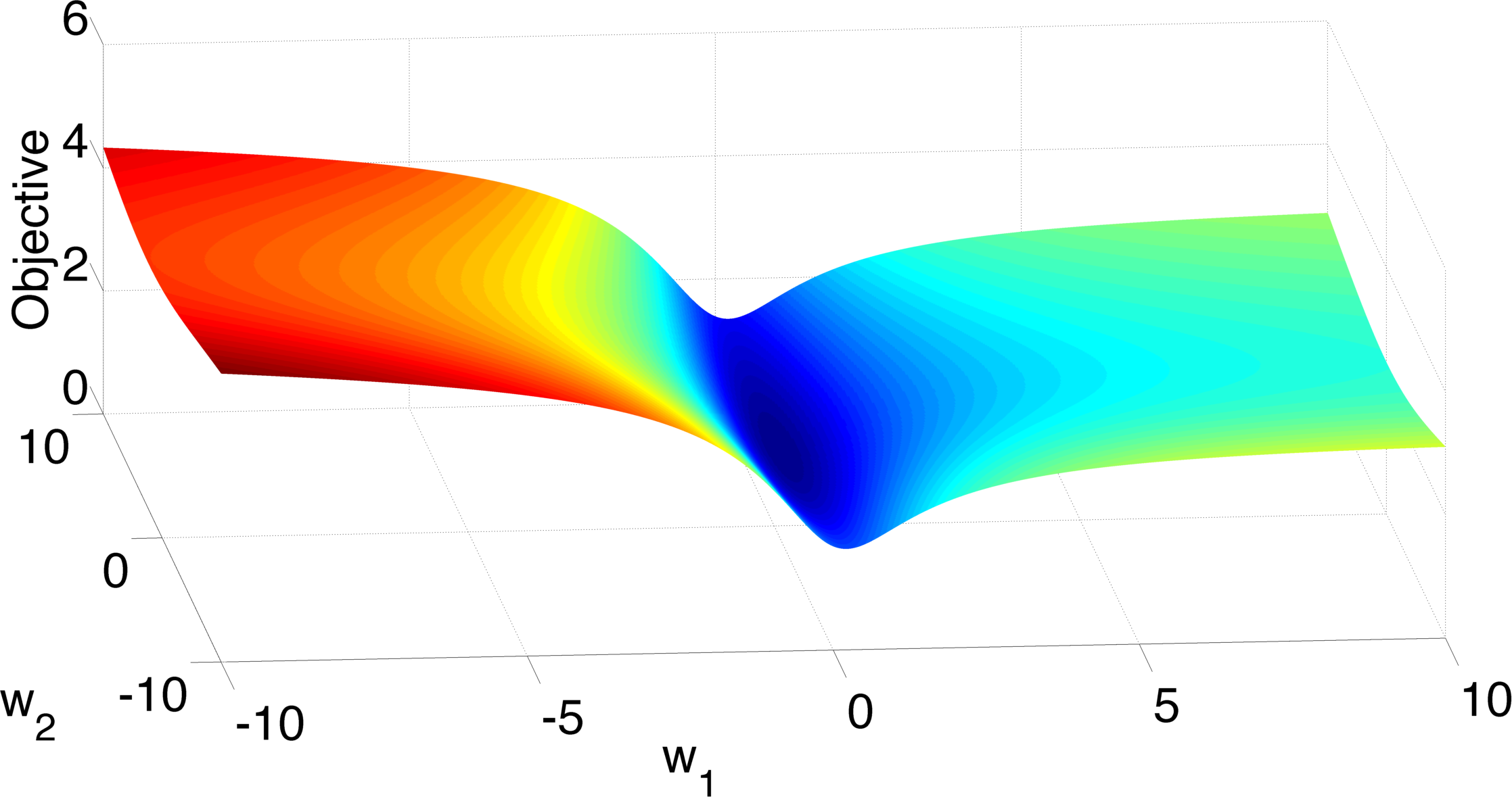
Figure 1: Risk values for various weight vectors $w=(w_{1},w_{2})$, TangentBoost, Long and Servedio (2010) dataset.

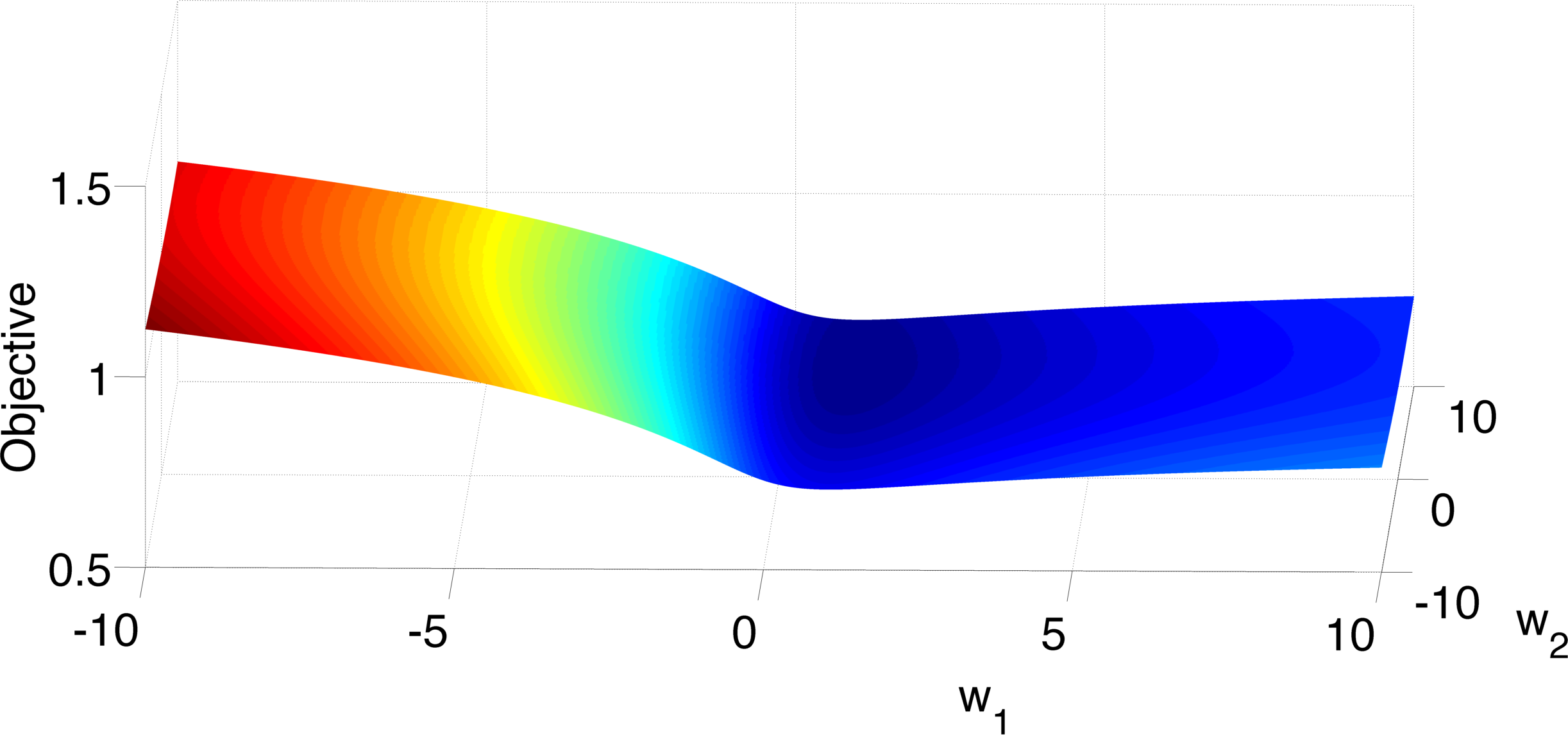
Figure 2: Risk values for various weight vectors $w=(w_{1},w_{2})$, $t$-logistic regression, Long and Servedio (2010) dataset.

The shape of these plots suggests that the minimiser is indeed found in the interval $[-10,10]^{2}$. To further verify this, we performed L-BFGS minimisation of these losses using $100$ different random initialisations, uniformly from $[-100,100]^{2}$. We find that in each trial, the TangentBoost solution converges to $w^{*}=(0.2122,1.3031)$, while the $t$-logistic solution converges to $w^{*}=(1.0372,5.0873)$, both of which result in accuracy of $\frac{1}{2}$ on $D$.

B.1 In defence of non-convex losses: beyond SLN-robustness

The above illustrates the possible non SLN-robustness of two non-convex losses. However, there may be other notions under which these losses are robust. For example, Ding and Vishwanathan (2010) defines robustness to be a stability of the asymptotic maximum likelihood solution when adding a new labelled instance (chosen arbitrarily from $\mathscr{X}\times\{\pm 1\}$), based on a definition in O’Hagan (1979). Intuitively, this captures robustness to outliers in the instance space, so that e.g. an adversarial mislabelling of an instance far from the true decision boundary does not adversely affect the learned model. Such a notion of robustness is clearly of practical interest, and future study of such alternate notions would be of value.

B.2 Conjecture: (most) strictly proper composite losses are not SLN-robust

More abstractly, we conjecture the above can be generalised to the following. Recall that a loss $\ell$ is strictly proper composite (Reid and Williamson, 2010) if its (unique) Bayes-optimal scorer is some strictly monotone transformation $\psi$ of the class-probability function: $(\forall D)\,\mathscr{S}^{D,*}_{\ell}=\{\psi\circ\eta\}.$

Conjecture 1.

Pick any strictly proper composite (but not necessarily convex) $\ell$ whose link function has range $\mathbb{R}$. Then, $(\ell,\mathscr{F}_{\mathrm{lin}})$ is not SLN-robust.

We believe the above is true for the following reason. Suppose $D$ is some linearly separable distribution, with $\eta\colon x\mapsto\llbracket\langle w^{*},x\rangle>0\rrbracket$ for some $w^{*}$. Then, minimising $\ell$ with $\mathscr{F}_{\mathrm{lin}}$ will be well-specified: the Bayes-optimal scorer is $\psi(\llbracket\langle w^{*},x\rangle>0\rrbracket)$. If the range of $\psi$ is $\mathbb{R}$, then this is equivalent to $\infty\cdot(2\llbracket\langle w^{*},x\rangle>0\rrbracket-1)$, which is in $\mathscr{F}_{\mathrm{lin}}$ if we allow for the extended reals. The resulting classifier will thus have $100\%$ accuracy.

However, by injecting any non-zero label noise, minimising $\ell$ with $\mathscr{F}_{\mathrm{lin}}$ will no longer be well-specified, as $\accentset{\rule{2.79996pt}{0.6pt}}{\eta}$ takes on the values $\{1-\rho,\rho\}$, which cannot be the sole set of output scores for any linear scorer if $|\mathscr{X}|>3$. We believe it unlikely that every such misspecified solution have $100\%$ accuracy on $D$. We further believe it likely that one can exhibit a scenario, possibly the same as the Long and Servedio (2010) example, where the resulting solution has accuracy 50%.

Two further comments are in order. First, if a loss is strictly proper composite, then it cannot satisfy Equation 6, and hence it cannot be strongly SLN-robust. (However, this does leave open the possibility that with $\mathscr{F}_{\mathrm{lin}}$, the loss is SLN-robust.) Second, observe that the restriction that $\psi$ have range $\mathbb{R}$ is necessary to rule out cases such as square loss, where the link function has range $[-1,1]$.

Appendix C Preservation of mean maps

Pick any $D$, and $\rho\in[0,1/2)$. Then,

$$(\forall x\in\mathscr{X})\,2\accentset{\rule{2.79996pt}{0.6pt}}{\eta}(x)-1 =2\cdot((1-2\rho)\cdot\eta(x)+\rho)-1$$

$$=(1-2\rho)\cdot(2\eta(x)-1).$$

Thus, for any feature mapping $\Phi\colon\mathscr{X}\to\mathscr{H}$, the kernel mean map of the clean distribution is

$$\underset{(\mathsf{X},\mathsf{Y})\sim D}{\mathbb{E}}\left[\mathsf{Y}\cdot\Phi(\mathsf{X})\right] =\underset{\mathsf{X}\sim M}{\mathbb{E}}\left[(2\eta(\mathsf{X})-1)\cdot\Phi(\mathsf{X})\right]$$

$$=\frac{1}{(1-2\rho}\cdot\underset{\mathsf{X}\sim M}{\mathbb{E}}\left[(2\accentset{\rule{2.79996pt}{0.6pt}}{\eta}(\mathsf{X})-1)\cdot\Phi(\mathsf{X})\right]$$

$$=\frac{1}{(1-2\rho)}\cdot\underset{(\mathsf{X},\mathsf{Y})\sim\mathrm{SLN}(D,\rho)}{\mathbb{E}}\left[\mathsf{Y}\cdot\Phi(\mathsf{X})\right],$$

which is a scaled version of the kernel mean map of the noisy distribution. That is, the kernel mean map is preserved under symmetric label noise. Instantiating the above with a specific instance $x\in\mathscr{X}$ gives Equation 10.

Appendix D Additional theoretical considerations

D.1 Generalisation bounds

Generalisation bounds are readily derived for the unhinged loss. For a training sample $\mathsf{S}\sim D^{n}$, define the $\ell$-deviation of a scorer $s\colon\mathscr{X}\to\mathbb{R}$ to be the difference in its population and empirical $\ell$-risk,

$$\text{dev}^{D,\mathsf{S}}_{\ell}(s)=\mathbb{L}^{D}_{\ell}(s)-\mathbb{L}^{\mathsf{S}}_{\ell}(s).$$

This quantity is of interest because a standard result says that for the empirical risk minimiser $s_{n}$ over some function class $\mathscr{F}$, $\mathrm{regret}^{D,\mathscr{F}}_{\ell}(s_{n})\leq 2\cdot\sup_{s\in\mathscr{F}}|\text{dev}^{D,\mathsf{S}}_{\ell}(s)|$ (Boucheron et al., 2005, Equation 2). For unhinged loss, we have the following Rademacher based bound.

Proposition 10.

Pick any $D$ and $n\in\mathbb{N}_{+}$. Let $\mathsf{S}\sim D^{n}$ denote an empirical sample. For some $B\in\mathbb{R}_{+}$, let $s\in\mathscr{F}_{B}$. Then, with probability at least $1-\delta$ over the choice of $\mathsf{S}$, for $\ell=\ell^{\mathrm{unh}}$,

$$\mathrm{dev}^{D,\mathsf{S}}_{\ell}(s)\leq 2\cdot\mathscr{R}_{n}(\mathscr{F}_{B},\mathsf{S})+B\cdot\sqrt{\frac{\log\frac{2}{\delta}}{2n}}$$

where $\mathscr{R}_{n}(\mathscr{F}_{B},\mathsf{S})$ is the empirical Rademacher complexity of $\mathscr{F}_{B}$ on sample $\mathsf{S}$.

Proof of Proposition 10.

The standard Rademacher-complexity generalisation bound (Bartlett and Mendelson, 2002, Theorem 7), (Boucheron et al., 2005, Theorem 4.1) states that with probability at least $1-\delta$ over the choice of $\mathsf{S}$,

$$\mathrm{dev}^{D,\mathsf{S}}_{\ell}(s)\leq 2\cdot||(\ell)^{\prime}||_{\infty}\cdot\mathscr{R}_{n}(\mathscr{F}_{B},\mathsf{S})+||\ell||_{\infty}\cdot\sqrt{\frac{\log\frac{2}{\delta}}{2n}}.$$

For the unhinged loss, $||(\ell^{\mathrm{unh}})^{\prime}||_{\infty}=1$. Further, since we work over bounded scorers, $||\ell^{\mathrm{unh}}||_{\infty}=B$. The result follows. ∎

Proposition 10 holds equally when learning from a corrupted sample $\bar{\mathsf{S}}\sim\accentset{\rule{2.79996pt}{0.6pt}}{D}^{n}$. Since $\mathrm{regret}^{D,\mathscr{F}}_{\ell^{\mathrm{unh}}}(s_{n})=\frac{1}{1-2\rho}\cdot\mathrm{regret}^{\accentset{\rule{2.79996pt}{0.6pt}}{D},\mathscr{F}}_{\ell^{\mathrm{unh}}}(s_{n})$ by Proposition 6, by minimising the unhinged loss on the corrupted sample, we can bound the regret on the clean distribution.

Appendix E Additional relations to existing methods

We discuss some further connections of the unhinged loss to existing methods.

E.1 Unhinging the SVM

We can motivate the unhinged loss intuitively by studying the noise-corrected versions of the hinge loss, as per Equation 4. Figure 3 shows the noise corrected hinge loss for $\rho\in\{0,0.2,0.4\}$. We see that as the noise rate increases, the effect is to slightly unhinge the original loss, by removing its flat portion. Thus, if we knew the noise rate $\rho$, we could use these slightly unhinged losses to learn.

Figure 3: Noise-corrected versions of hinge loss, $\ell_{1}(v)=\max(0,1-v)$. Best viewed in colour.

Of course, in general we do not know the noise rate. Further, the slightly unhinged losses are non-convex. So, in order to be robust to an arbitrary noise rate $\rho$, we can completely unhinge the loss, yielding

$$\ell^{\mathrm{unh}}_{1}(v) =1-v\text{ and }\ell^{\mathrm{unh}}_{-1}(v)=1+v.$$

E.2 Relation to centroid classifiers

As established in §6.1, the optimal unhinged classifier (Equation 9) is equivalent to a centroid classifier, where one replaces the positive and negative classes by their centroids, and performs classification based on the distance of an instance to the two centroids. Such a classifier has been proposed as a prototypical example of a simple kernel-based classifier (Schölkopf and Smola, 2002, Section 1.2), (Shawe-Taylor and Cristianini, 2004, Section 5.1) Balcan et al. (2008, Definition 4) considers such classification rules using general similarity functions in place of kernels corresponding to an RKHS.

The optimal unhinged classifier is also closely related to the Rocchio classifier in information retrieval (Manning et al., 2008, pg. 181), and the nearest centroid classifier in computational genomics (Tibshirani et al., 2002). The optimal kernelised scorer for these approaches is (Doloc-Mihu et al., 2003)

$$s^{*}\colon x\mapsto\left(\underset{\mathsf{X}\sim P}{\mathbb{E}}\left[k(\mathsf{X},x)\right]-\underset{\mathsf{X}\sim Q}{\mathbb{E}}\left[k(\mathsf{X},x)\right]\right),$$

i.e. it does not weight each of the kernel means.

E.3 Relation to kernel density estimation

When working with an RKHS with a translation invariant kernel, the optimal unhinged scorer (Equation 9) can be interpreted as follows: perform kernel density estimation on the positive and negative classes, and then classify instances according to Bayes’ rule. For example, with a Gaussian RBF kernel, the classifier is equivalent to using a Gaussian kernel to compute density estimates of $P,Q$, and using these to classify. This is known as a kernel classification rule (Devroye et al., 1996, Chapter 10).

This perspective suggests that in computing $s^{*}_{\mathrm{unh},\lambda}$, we may also estimate the corrupted class-probability function. In particular, observe that if we compute $\frac{\pi}{1-\pi}\cdot\frac{\underset{\mathsf{X}\sim P}{\mathbb{E}}\left[k(\mathsf{X},x)\right]}{\underset{\mathsf{X}\sim Q}{\mathbb{E}}\left[k(\mathsf{X},x)\right]}$, similar to the Nadaraya-Watson estimator (Bishop, 2006, pg. 300), then this provides an estimate of $\frac{\eta(x)}{1-\eta(x)}$. Of course, such an approach will succumb to the curse of dimensionality.

An alternative is to use the Probing reduction (Langford and Zadrozny, 2005), by computing an ensemble of cost-sensitive classifiers at varying cost ratios. To this end, observe that the following weighted unhinged (or whinge) loss,

$$\ell^{\mathrm{whinge}}_{1}(v) =c_{1}\cdot-v$$

$$\ell^{\mathrm{whinge}}_{-1}(v) =c_{-1}\cdot v$$

for some $c_{-1}\in[0,1]$ and $c_{1}=1-c_{-1}$, will have a restricted Bayes-optimal scorer of $B\cdot\operatorname{sign}(\eta(x)-{c_{-1}})$ over $\mathscr{F}_{B}$. Further, it will result in an optimal scorer that simply weights each of the kernel means,

$$s^{*}_{\mathrm{whinge},\lambda}\colon x\mapsto\frac{1}{\lambda}\cdot\underset{(\mathsf{X},\mathsf{Y})\sim D}{\mathbb{E}}\left[c_{\mathsf{Y}}\cdot\mathsf{Y}\cdot k(\mathsf{X},x)\right],$$

making it trivial to compute as $c$ is varied.

E.4 Relation to the MMD witness

The optimal weight vector for unhinged loss (Equation 8) can be expressed as

$$w^{*}_{\mathrm{unh},\lambda}=\frac{1}{\lambda}\cdot({\pi}\cdot\mu_{P}-(1-{\pi})\cdot\mu_{Q}),$$

where $\mu_{P}$ and $\mu_{Q}$ are the kernel mean maps with respect to $\mathscr{H}$ of the positive and negative class-conditionals distributions,

$$\mu_{P} =\underset{\mathsf{X}\sim P}{\mathbb{E}}\left[\Phi(\mathsf{X})\right]$$

$$\mu_{Q} =\underset{\mathsf{X}\sim Q}{\mathbb{E}}\left[\Phi(\mathsf{X})\right].$$

When $\pi=\frac{1}{2}$, $||w^{*}_{1}||_{\mathscr{H}}$ is precisely the maximum mean discrepancy (MMD) (Gretton et al., 2012) between $P$ and $Q$, using all functions in the unit ball of $\mathscr{H}$. The mapping $x\mapsto\langle w^{*}_{1},x\rangle_{\mathscr{H}}$ itself is referred to as the witness function (Gretton et al., 2012, §2.3). While the motivation of MMD is to perform hypothesis testing so as to distinguish between two distributions $P,Q$, rather than constructing a suitable scorer, the fact that it arises from the optimal scorer for the unhinged loss has been previously noted (Sriperumbudur et al., 2009, Theorem 1).

Appendix F Example of poor classification with square loss

We illustrate that square loss with a linear function class may perform poorly even when the underlying distribution is linearly separable. We consider the dataset of Long and Servedio (2010), with no label noise. That is, we have $\mathscr{X}=\{(1,0),(\gamma,5\gamma),(\gamma,-\gamma),(\gamma,-\gamma)\}\subset\mathbb{R}^{2}$, and $\eta\colon x\mapsto 1$. Let $X\in\mathbb{R}^{4\times 2}$ be the feature matrix of the four data points. Then, the optimal weight vector learned by square loss is

$$w^{*} =(X^{T}X)^{-1}X^{T}\begin{bmatrix}1\\ 1\\ 1\\ 1\end{bmatrix}$$

$$=\begin{bmatrix}\frac{8\gamma+3}{8\gamma^{2}+3}\\ -\frac{\gamma+1}{3\gamma\cdot(8\gamma^{2}+3)}\end{bmatrix}.$$

It is easy to check that the predicted scores are then

$$s^{*}=\begin{bmatrix}\frac{8\gamma+3}{8\gamma^{2}+3}\\ \frac{\gamma\cdot(8\gamma+3)}{8\gamma^{2}+3-\frac{5\cdot(\gamma-1)\gamma}{24\gamma^{3}+9\gamma}}\\ \frac{(\gamma-1)\cdot\gamma}{24\gamma^{3}+9\gamma+\frac{\gamma\cdot(8\gamma+3)}{8\gamma^{2}+3}}\\ \frac{(\gamma-1)\cdot\gamma}{24\gamma^{3}+9\gamma+\frac{\gamma\cdot(8\gamma+3)}{8\gamma^{2}+3}}\end{bmatrix}.$$

But for $\gamma<\frac{1}{12}$, this means that the predicted scores for the last two examples are negative. That is, the resulting classifier will have $50\%$ accuracy. (This does not contradict the robustness of square loss, as robustness simply requires that performance is the same with and without noise.)

It is initially surprising that square loss fails in this example, as we are employing a linear function class, and the true $\eta$ is expressible as a linear function. However, recall that the Bayes-optimal scorer for square loss is

$$\mathscr{S}^{D,*}_{\ell}=\{s\colon x\mapsto 2\eta(x)-1\}.$$

In this case, the Bayes-optimal scorer is

$$s^{*}\colon x\mapsto 2\llbracket x_{1}>0\rrbracket-1.$$

The application of a threshold means the that scorer is not expressible as a linear model. Therefore, the combination of loss and function class is in fact not well-specified for the problem.

To clarify this point, consider the use of the squared hinge loss, $\ell(y,v)=\max(0,1-yv)^{2}$. This loss induces a set of Bayes-optimal scorers, which are:

$$\mathscr{S}^{D,*}_{\ell}=\left\{s\mid(\forall x\in\mathscr{X})\,\begin{cases}\eta(x)=1&\implies s(x)\in[1,\infty)\\ \eta(x)\in(0,1)&\implies s(x)=2\eta(x)-1\\ \eta(x)=0&\implies s(x)\in(-\infty,1].\end{cases}\right\}$$

Crucially, we can find a linear scorer that is in this set: for, say, $v=(\frac{1}{\gamma},0)$, we clearly have $\langle v,x\rangle\geq 1$ for every $x\in\mathscr{X}$, and so this is a Bayes-optimal scorer. Thus, minimising the square hinge loss on this distribution will indeed find a classifier with $100\%$ accuracy.

Appendix G Example of poor classification with unhinged loss

We illustrate that the unhinged loss with a linear function class may perform poorly even when the underlying distribution is linearly separable. (For another example where instances are on the unit ball, see Balcan et al. (2008, Figure 1).) Consider a distribution $D_{M,\eta}$ uniformly concentrated on $\mathscr{X}=\{x_{1},x_{2},x_{3}\}$ with $x_{1}=(1,2),x_{2}=(1,-4),x_{3}=(-1,1)$, with $\eta(x_{1})=\eta(x_{2})=1$ and $\eta(x_{3})=0$, i.e. the first two instances are positive, and the third instance negative. Then it is evident that the optimal unhinged hyperplane, with regularisation strength 1, is $w^{*}=(1,-1)$. This will misclassify the first instance as being negative. Figure 4 illustrates.

It is easy to check that for this particular distribution, the optimal weight for square loss is $w^{*}=(1,0)$. This results in perfect classification. Thus, we have a reversal of the scenario of the previous section – here, square loss classifies perfectly, while the unhinged loss classifies no better than random guessing.

It may appear that the above contradicts the classification-calibration of the unhinged loss: there certainly is a linear scorer that is Bayes-optimal over $\mathscr{F}_{B}$, namely, $w^{*}=(B,0)$. The subtlety is that in this case, minimisation over the unit ball $||w||_{2}\leq 1$ (as implied by $\ell_{2}$ regularisation) is unable to restrict attention to the desired scorer.

There are two ways to rectify examples such as the above. First, as in general, we can employ a suitably rich kernel, e.g. a Gaussian RBF kernel. It is not hard to verify that on this dataset, such a kernel will find a perfect classifier. Second, we can look to explicitly enforce that minimisation is over all $w$ satisfying $|\langle w,x_{n}\rangle|\leq 1$. This will result in a linear program (LP) that may be solved easily, but does not admit a closed form solution as in the case of minimising over the unit ball. It may be checked that the resulting LP will recover the optimal weight $w^{*}=(1,0)$. While this approach is suitable for this particular example, issues arise when dealing with infinite dimensional feature mappings (as we lose the existence of a representer theorem without regularisation based on the norm in the Hilbert space (Yu et al., 2013)).

Figure 4: Example of linearly separable distribution where, when learning with the unhinged loss and a linear function class, the resulting hyperplane (in red) misclassifies one of the instances.

Additional Experiments for “Learning with Symmetric Label Noise: The Importance of Being Unhinged”

Appendix H Additional experimental results

Table 3 reports the 0-1 error for a range of losses on the Long and Servedio (2010) dataset. TanBoost refers to the loss of Masnadi-Shirazi et al. (2010). As before, we find the unhinged loss to generally find a good classifier. Observe that the relatively poor performance of the square and TanBoost loss can be attributed to the findings of Appendix B, F.

We next report the 0-1 error and one minus the AUC for a range of datasets. We begin with a dataset of Mease and Wyner (2008), where $\mathscr{X}=[0,1]^{20}$, and $M$ is the uniform distribution. Further, we have $\eta\colon x\mapsto\llbracket\langle w^{*},x\rangle>2.5\rrbracket$ for $w^{*}=\begin{bmatrix}\mathbf{1}_{5}&\mathbf{0}_{15}\end{bmatrix}$, i.e. there is a sparse separating hyperplane. Table 4 reports the results on this dataset injected with various levels of symmetric noise. On this dataset, the $t$-logistic loss generally performs the best.

Finally, we report the 0-1 error and one minus the AUC on some UCI datasets in Tables 5 – 6. Table 2 summarises statistics of the UCI data. Several datasets are imbalanced, meaning that 0-1 error is not the ideal measure of performance (as it can be made small with a trivial majority classifier). The AUC is thus arguably a better indication of performance for these datasets. We generally find that at high noise rates (40%), the AUC of the unhinged loss is superior to that of other losses.

Dataset	$N$	$D$	$\mathbb{P}(\mathsf{Y}=1)$
Iris	150	4	0.3333
Ionosphere	351	34	0.3590
Housing	506	13	0.0692
Car	1,728	8	0.0376
USPS 0v7	2,200	256	0.5000
Splice	3,190	61	0.2404
Spambase	4,601	57	0.3940

Table 2: Summary of UCI datasets. Here, $N$ denotes the total number of samples, and $D$ the dimensionality of the feature space.

	Hinge	Logistic	Square	$t$-logistic	TanBoost	Unhinged
$\rho=0$	0.00 $\pm$ 0.00	0.00 $\pm$ 0.00	0.25 $\pm$ 0.00	0.00 $\pm$ 0.00	0.25 $\pm$ 0.00	0.00 $\pm$ 0.00
$\rho=0.1$	0.15 $\pm$ 0.27	0.24 $\pm$ 0.05	0.25 $\pm$ 0.00	0.00 $\pm$ 0.00	0.25 $\pm$ 0.00	0.00 $\pm$ 0.00
$\rho=0.2$	0.21 $\pm$ 0.30	0.25 $\pm$ 0.00	0.25 $\pm$ 0.00	0.00 $\pm$ 0.00	0.25 $\pm$ 0.00	0.00 $\pm$ 0.00
$\rho=0.3$	0.38 $\pm$ 0.37	0.25 $\pm$ 0.03	0.25 $\pm$ 0.02	0.22 $\pm$ 0.08	0.25 $\pm$ 0.03	0.00 $\pm$ 0.00
$\rho=0.4$	0.42 $\pm$ 0.36	0.22 $\pm$ 0.08	0.22 $\pm$ 0.08	0.22 $\pm$ 0.08	0.22 $\pm$ 0.08	0.00 $\pm$ 0.00
$\rho=0.49$	0.46 $\pm$ 0.38	0.39 $\pm$ 0.23	0.39 $\pm$ 0.23	0.39 $\pm$ 0.23	0.39 $\pm$ 0.23	0.34 $\pm$ 0.48

Table 3: Results on Long and Servedio (2010) dataset. Reported is the mean and standard deviation of the 0-1 error over 125 trials. Grayed cells denote the best performer at that noise rate.

	Hinge	Logistic	Square	$t$-logistic	TanBoost	Unhinged
$\rho=0$	0.02 $\pm$ 0.00	0.01 $\pm$ 0.00	0.03 $\pm$ 0.00	0.01 $\pm$ 0.00	0.02 $\pm$ 0.00	0.05 $\pm$ 0.00
$\rho=0.1$	0.13 $\pm$ 0.01	0.05 $\pm$ 0.01	0.06 $\pm$ 0.01	0.03 $\pm$ 0.01	0.05 $\pm$ 0.01	0.06 $\pm$ 0.01
$\rho=0.2$	0.14 $\pm$ 0.01	0.09 $\pm$ 0.02	0.09 $\pm$ 0.02	0.06 $\pm$ 0.02	0.08 $\pm$ 0.02	0.08 $\pm$ 0.02
$\rho=0.3$	0.15 $\pm$ 0.01	0.13 $\pm$ 0.03	0.13 $\pm$ 0.03	0.12 $\pm$ 0.03	0.12 $\pm$ 0.03	0.12 $\pm$ 0.02
$\rho=0.4$	0.17 $\pm$ 0.05	0.24 $\pm$ 0.08	0.24 $\pm$ 0.08	0.23 $\pm$ 0.07	0.23 $\pm$ 0.08	0.23 $\pm$ 0.08
$\rho=0.49$	0.47 $\pm$ 0.24	0.46 $\pm$ 0.11	0.47 $\pm$ 0.11	0.48 $\pm$ 0.10	0.47 $\pm$ 0.12	0.48 $\pm$ 0.12

(a) 0-1 Error.

	Hinge	Logistic	Square	$t$-logistic	TanBoost	Unhinged
$\rho=0$	0.00 $\pm$ 0.00	0.00 $\pm$ 0.00	0.01 $\pm$ 0.00	0.00 $\pm$ 0.00	0.00 $\pm$ 0.00	0.01 $\pm$ 0.00
$\rho=0.1$	0.25 $\pm$ 0.10	0.02 $\pm$ 0.01	0.02 $\pm$ 0.01	0.00 $\pm$ 0.00	0.02 $\pm$ 0.01	0.02 $\pm$ 0.01
$\rho=0.2$	0.34 $\pm$ 0.10	0.05 $\pm$ 0.02	0.05 $\pm$ 0.02	0.02 $\pm$ 0.01	0.04 $\pm$ 0.02	0.05 $\pm$ 0.02
$\rho=0.3$	0.41 $\pm$ 0.11	0.11 $\pm$ 0.04	0.11 $\pm$ 0.04	0.09 $\pm$ 0.04	0.11 $\pm$ 0.04	0.10 $\pm$ 0.04
$\rho=0.4$	0.44 $\pm$ 0.12	0.24 $\pm$ 0.08	0.24 $\pm$ 0.08	0.24 $\pm$ 0.08	0.24 $\pm$ 0.08	0.23 $\pm$ 0.08
$\rho=0.49$	0.50 $\pm$ 0.13	0.47 $\pm$ 0.11	0.47 $\pm$ 0.11	0.47 $\pm$ 0.11	0.47 $\pm$ 0.11	0.46 $\pm$ 0.11

(b) 1 - AUC.

Table 4: Results on mease dataset. Reported is the mean and standard deviation of performance over 125 trials. Grayed cells denote the best performer at that noise rate.

	Hinge	Logistic	Square	$t$-logistic	TanBoost	Unhinged
$\rho=0$	0.00 $\pm$ 0.00	0.00 $\pm$ 0.00	0.00 $\pm$ 0.00	0.00 $\pm$ 0.00	0.00 $\pm$ 0.00	0.00 $\pm$ 0.00
$\rho=0.1$	0.01 $\pm$ 0.03	0.01 $\pm$ 0.01	0.01 $\pm$ 0.02	0.01 $\pm$ 0.03	0.01 $\pm$ 0.02	0.00 $\pm$ 0.00
$\rho=0.2$	0.06 $\pm$ 0.12	0.02 $\pm$ 0.05	0.03 $\pm$ 0.04	0.04 $\pm$ 0.05	0.03 $\pm$ 0.05	0.00 $\pm$ 0.01
$\rho=0.3$	0.17 $\pm$ 0.20	0.09 $\pm$ 0.10	0.08 $\pm$ 0.09	0.09 $\pm$ 0.11	0.09 $\pm$ 0.10	0.02 $\pm$ 0.07
$\rho=0.4$	0.35 $\pm$ 0.24	0.24 $\pm$ 0.17	0.24 $\pm$ 0.17	0.24 $\pm$ 0.16	0.24 $\pm$ 0.17	0.13 $\pm$ 0.22
$\rho=0.49$	0.60 $\pm$ 0.20	0.49 $\pm$ 0.20	0.49 $\pm$ 0.19	0.49 $\pm$ 0.20	0.49 $\pm$ 0.19	0.45 $\pm$ 0.33

(a) 0-1 Error.

	Hinge	Logistic	Square	$t$-logistic	TanBoost	Unhinged
$\rho=0$	0.00 $\pm$ 0.00	0.00 $\pm$ 0.00	0.00 $\pm$ 0.00	0.00 $\pm$ 0.00	0.00 $\pm$ 0.00	0.00 $\pm$ 0.00
$\rho=0.1$	0.00 $\pm$ 0.00	0.00 $\pm$ 0.00	0.00 $\pm$ 0.00	0.00 $\pm$ 0.00	0.00 $\pm$ 0.00	0.00 $\pm$ 0.00
$\rho=0.2$	0.03 $\pm$ 0.11	0.00 $\pm$ 0.01	0.00 $\pm$ 0.00	0.00 $\pm$ 0.01	0.00 $\pm$ 0.01	0.00 $\pm$ 0.00
$\rho=0.3$	0.14 $\pm$ 0.26	0.02 $\pm$ 0.06	0.02 $\pm$ 0.05	0.02 $\pm$ 0.06	0.02 $\pm$ 0.05	0.01 $\pm$ 0.06
$\rho=0.4$	0.36 $\pm$ 0.38	0.13 $\pm$ 0.18	0.13 $\pm$ 0.18	0.14 $\pm$ 0.18	0.13 $\pm$ 0.18	0.09 $\pm$ 0.27
$\rho=0.49$	0.72 $\pm$ 0.34	0.47 $\pm$ 0.31	0.48 $\pm$ 0.30	0.48 $\pm$ 0.30	0.48 $\pm$ 0.30	0.45 $\pm$ 0.48

(b) 1 - AUC.

Table 5: Results on iris dataset. Reported is the mean and standard deviation of performance over 125 trials. Grayed cells denote the best performer at that noise rate.

	Hinge	Logistic	Square	$t$-logistic	TanBoost	Unhinged
$\rho=0$	0.11 $\pm$ 0.00	0.13 $\pm$ 0.00	0.17 $\pm$ 0.00	0.24 $\pm$ 0.00	0.17 $\pm$ 0.00	0.20 $\pm$ 0.00
$\rho=0.1$	0.17 $\pm$ 0.04	0.18 $\pm$ 0.04	0.16 $\pm$ 0.03	0.19 $\pm$ 0.05	0.17 $\pm$ 0.04	0.19 $\pm$ 0.02
$\rho=0.2$	0.20 $\pm$ 0.05	0.19 $\pm$ 0.05	0.18 $\pm$ 0.04	0.21 $\pm$ 0.06	0.18 $\pm$ 0.04	0.19 $\pm$ 0.02
$\rho=0.3$	0.23 $\pm$ 0.06	0.22 $\pm$ 0.05	0.22 $\pm$ 0.05	0.24 $\pm$ 0.06	0.22 $\pm$ 0.05	0.21 $\pm$ 0.03
$\rho=0.4$	0.31 $\pm$ 0.11	0.31 $\pm$ 0.10	0.29 $\pm$ 0.09	0.32 $\pm$ 0.09	0.30 $\pm$ 0.10	0.27 $\pm$ 0.12
$\rho=0.49$	0.48 $\pm$ 0.16	0.47 $\pm$ 0.16	0.47 $\pm$ 0.16	0.47 $\pm$ 0.14	0.45 $\pm$ 0.15	0.46 $\pm$ 0.22

(a) 0-1 Error.

	Hinge	Logistic	Square	$t$-logistic	TanBoost	Unhinged
$\rho=0$	0.12 $\pm$ 0.00	0.13 $\pm$ 0.00	0.07 $\pm$ 0.00	0.20 $\pm$ 0.00	0.07 $\pm$ 0.00	0.21 $\pm$ 0.00
$\rho=0.1$	0.18 $\pm$ 0.07	0.18 $\pm$ 0.07	0.12 $\pm$ 0.04	0.22 $\pm$ 0.07	0.13 $\pm$ 0.05	0.21 $\pm$ 0.00
$\rho=0.2$	0.23 $\pm$ 0.09	0.22 $\pm$ 0.09	0.18 $\pm$ 0.07	0.25 $\pm$ 0.08	0.19 $\pm$ 0.08	0.21 $\pm$ 0.01
$\rho=0.3$	0.31 $\pm$ 0.11	0.29 $\pm$ 0.09	0.26 $\pm$ 0.09	0.30 $\pm$ 0.09	0.27 $\pm$ 0.09	0.21 $\pm$ 0.01
$\rho=0.4$	0.40 $\pm$ 0.11	0.40 $\pm$ 0.10	0.38 $\pm$ 0.10	0.40 $\pm$ 0.10	0.38 $\pm$ 0.10	0.25 $\pm$ 0.12
$\rho=0.49$	0.49 $\pm$ 0.12	0.50 $\pm$ 0.10	0.50 $\pm$ 0.10	0.50 $\pm$ 0.10	0.50 $\pm$ 0.10	0.46 $\pm$ 0.25

(b) 1 - AUC.

Table 6: Results on ionosphere dataset. Reported is the mean and standard deviation of performance over 125 trials. Grayed cells denote the best performer at that noise rate.

	Hinge	Logistic	Square	$t$-logistic	TanBoost	Unhinged
$\rho=0$	0.05 $\pm$ 0.00	0.05 $\pm$ 0.00	0.07 $\pm$ 0.00	0.05 $\pm$ 0.00	0.07 $\pm$ 0.00	0.05 $\pm$ 0.00
$\rho=0.1$	0.06 $\pm$ 0.01	0.06 $\pm$ 0.02	0.07 $\pm$ 0.02	0.07 $\pm$ 0.02	0.07 $\pm$ 0.02	0.05 $\pm$ 0.00
$\rho=0.2$	0.06 $\pm$ 0.01	0.07 $\pm$ 0.03	0.07 $\pm$ 0.02	0.08 $\pm$ 0.03	0.07 $\pm$ 0.02	0.05 $\pm$ 0.00
$\rho=0.3$	0.08 $\pm$ 0.04	0.10 $\pm$ 0.06	0.11 $\pm$ 0.06	0.11 $\pm$ 0.05	0.11 $\pm$ 0.06	0.05 $\pm$ 0.01
$\rho=0.4$	0.14 $\pm$ 0.10	0.21 $\pm$ 0.12	0.22 $\pm$ 0.12	0.24 $\pm$ 0.13	0.22 $\pm$ 0.13	0.09 $\pm$ 0.10
$\rho=0.49$	0.45 $\pm$ 0.26	0.49 $\pm$ 0.16	0.50 $\pm$ 0.16	0.49 $\pm$ 0.16	0.51 $\pm$ 0.17	0.46 $\pm$ 0.30

(a) 0-1 Error.

	Hinge	Logistic	Square	$t$-logistic	TanBoost	Unhinged
$\rho=0$	0.25 $\pm$ 0.00	0.15 $\pm$ 0.00	0.17 $\pm$ 0.00	0.25 $\pm$ 0.00	0.17 $\pm$ 0.00	0.69 $\pm$ 0.00
$\rho=0.1$	0.38 $\pm$ 0.12	0.27 $\pm$ 0.07	0.27 $\pm$ 0.07	0.30 $\pm$ 0.09	0.27 $\pm$ 0.07	0.69 $\pm$ 0.00
$\rho=0.2$	0.41 $\pm$ 0.13	0.35 $\pm$ 0.10	0.35 $\pm$ 0.10	0.35 $\pm$ 0.10	0.35 $\pm$ 0.10	0.68 $\pm$ 0.00
$\rho=0.3$	0.44 $\pm$ 0.12	0.40 $\pm$ 0.11	0.40 $\pm$ 0.11	0.40 $\pm$ 0.11	0.40 $\pm$ 0.11	0.69 $\pm$ 0.01
$\rho=0.4$	0.43 $\pm$ 0.12	0.45 $\pm$ 0.12	0.45 $\pm$ 0.12	0.45 $\pm$ 0.12	0.45 $\pm$ 0.12	0.68 $\pm$ 0.02
$\rho=0.49$	0.45 $\pm$ 0.13	0.49 $\pm$ 0.13	0.49 $\pm$ 0.13	0.49 $\pm$ 0.13	0.49 $\pm$ 0.13	0.57 $\pm$ 0.16

(b) 1 - AUC.

Table 7: Results on housing dataset. Reported is the mean and standard deviation of performance over 125 trials. Grayed cells denote the best performer at that noise rate.

	Hinge	Logistic	Square	$t$-logistic	TanBoost	Unhinged
$\rho=0$	0.01 $\pm$ 0.00	0.02 $\pm$ 0.00	0.03 $\pm$ 0.00	0.03 $\pm$ 0.00	0.02 $\pm$ 0.00	0.03 $\pm$ 0.00
$\rho=0.1$	0.05 $\pm$ 0.00	0.04 $\pm$ 0.01	0.04 $\pm$ 0.01	0.02 $\pm$ 0.01	0.04 $\pm$ 0.01	0.04 $\pm$ 0.01
$\rho=0.2$	0.05 $\pm$ 0.00	0.05 $\pm$ 0.01	0.05 $\pm$ 0.01	0.04 $\pm$ 0.01	0.05 $\pm$ 0.01	0.05 $\pm$ 0.01
$\rho=0.3$	0.05 $\pm$ 0.01	0.06 $\pm$ 0.01	0.06 $\pm$ 0.01	0.06 $\pm$ 0.02	0.06 $\pm$ 0.01	0.06 $\pm$ 0.01
$\rho=0.4$	0.06 $\pm$ 0.02	0.11 $\pm$ 0.06	0.11 $\pm$ 0.06	0.11 $\pm$ 0.06	0.11 $\pm$ 0.06	0.10 $\pm$ 0.05
$\rho=0.49$	0.33 $\pm$ 0.27	0.46 $\pm$ 0.16	0.46 $\pm$ 0.16	0.47 $\pm$ 0.16	0.47 $\pm$ 0.16	0.46 $\pm$ 0.16

(a) 0-1 Error.

	Hinge	Logistic	Square	$t$-logistic	TanBoost	Unhinged
$\rho=0$	0.00 $\pm$ 0.00	0.00 $\pm$ 0.00	0.01 $\pm$ 0.00	0.00 $\pm$ 0.00	0.01 $\pm$ 0.00	0.02 $\pm$ 0.00
$\rho=0.1$	0.34 $\pm$ 0.18	0.03 $\pm$ 0.02	0.03 $\pm$ 0.02	0.00 $\pm$ 0.00	0.03 $\pm$ 0.02	0.04 $\pm$ 0.02
$\rho=0.2$	0.40 $\pm$ 0.17	0.07 $\pm$ 0.05	0.08 $\pm$ 0.05	0.04 $\pm$ 0.04	0.07 $\pm$ 0.05	0.08 $\pm$ 0.05
$\rho=0.3$	0.43 $\pm$ 0.17	0.17 $\pm$ 0.10	0.17 $\pm$ 0.10	0.14 $\pm$ 0.10	0.16 $\pm$ 0.10	0.16 $\pm$ 0.10
$\rho=0.4$	0.44 $\pm$ 0.18	0.30 $\pm$ 0.16	0.30 $\pm$ 0.16	0.30 $\pm$ 0.16	0.30 $\pm$ 0.16	0.30 $\pm$ 0.16
$\rho=0.49$	0.51 $\pm$ 0.19	0.46 $\pm$ 0.17	0.46 $\pm$ 0.17	0.46 $\pm$ 0.17	0.46 $\pm$ 0.17	0.46 $\pm$ 0.18

(b) 1 - AUC.

Table 8: Results on car dataset. Reported is the mean and standard deviation of performance over 125 trials. Grayed cells denote the best performer at that noise rate.

	Hinge	Logistic	Square	$t$-logistic	TanBoost	Unhinged
$\rho=0$	0.00 $\pm$ 0.00	0.00 $\pm$ 0.00	0.00 $\pm$ 0.00	0.00 $\pm$ 0.00	0.00 $\pm$ 0.00	0.00 $\pm$ 0.00
$\rho=0.1$	0.10 $\pm$ 0.08	0.05 $\pm$ 0.01	0.01 $\pm$ 0.01	0.11 $\pm$ 0.02	0.02 $\pm$ 0.01	0.00 $\pm$ 0.00
$\rho=0.2$	0.19 $\pm$ 0.11	0.09 $\pm$ 0.02	0.05 $\pm$ 0.02	0.15 $\pm$ 0.02	0.06 $\pm$ 0.02	0.00 $\pm$ 0.00
$\rho=0.3$	0.31 $\pm$ 0.13	0.17 $\pm$ 0.03	0.14 $\pm$ 0.02	0.22 $\pm$ 0.03	0.16 $\pm$ 0.03	0.01 $\pm$ 0.00
$\rho=0.4$	0.39 $\pm$ 0.13	0.31 $\pm$ 0.04	0.30 $\pm$ 0.04	0.33 $\pm$ 0.04	0.31 $\pm$ 0.04	0.02 $\pm$ 0.02
$\rho=0.49$	0.50 $\pm$ 0.16	0.48 $\pm$ 0.04	0.47 $\pm$ 0.04	0.48 $\pm$ 0.04	0.48 $\pm$ 0.04	0.34 $\pm$ 0.21

(a) 0-1 Error.

	Hinge	Logistic	Square	$t$-logistic	TanBoost	Unhinged
$\rho=0$	0.00 $\pm$ 0.00	0.00 $\pm$ 0.00	0.00 $\pm$ 0.00	0.00 $\pm$ 0.00	0.00 $\pm$ 0.00	0.00 $\pm$ 0.00
$\rho=0.1$	0.05 $\pm$ 0.06	0.01 $\pm$ 0.00	0.00 $\pm$ 0.00	0.05 $\pm$ 0.01	0.00 $\pm$ 0.00	0.00 $\pm$ 0.00
$\rho=0.2$	0.12 $\pm$ 0.11	0.03 $\pm$ 0.01	0.01 $\pm$ 0.00	0.07 $\pm$ 0.01	0.02 $\pm$ 0.01	0.00 $\pm$ 0.00
$\rho=0.3$	0.26 $\pm$ 0.18	0.10 $\pm$ 0.02	0.07 $\pm$ 0.02	0.14 $\pm$ 0.03	0.08 $\pm$ 0.02	0.00 $\pm$ 0.00
$\rho=0.4$	0.37 $\pm$ 0.19	0.25 $\pm$ 0.04	0.24 $\pm$ 0.04	0.27 $\pm$ 0.04	0.24 $\pm$ 0.04	0.00 $\pm$ 0.00
$\rho=0.49$	0.51 $\pm$ 0.23	0.47 $\pm$ 0.05	0.46 $\pm$ 0.05	0.47 $\pm$ 0.05	0.47 $\pm$ 0.05	0.25 $\pm$ 0.29

(b) 1 - AUC.

Table 9: Results on usps_0_vs_7 dataset. Reported is the mean and standard deviation of performance over 125 trials. Grayed cells denote the best performer at that noise rate.

	Hinge	Logistic	Square	$t$-logistic	TanBoost	Unhinged
$\rho=0$	0.05 $\pm$ 0.00	0.04 $\pm$ 0.00	0.02 $\pm$ 0.00	0.04 $\pm$ 0.00	0.02 $\pm$ 0.00	0.19 $\pm$ 0.00
$\rho=0.1$	0.15 $\pm$ 0.03	0.05 $\pm$ 0.01	0.04 $\pm$ 0.01	0.24 $\pm$ 0.00	0.04 $\pm$ 0.01	0.19 $\pm$ 0.01
$\rho=0.2$	0.21 $\pm$ 0.03	0.08 $\pm$ 0.01	0.07 $\pm$ 0.01	0.24 $\pm$ 0.00	0.07 $\pm$ 0.01	0.19 $\pm$ 0.01
$\rho=0.3$	0.25 $\pm$ 0.03	0.14 $\pm$ 0.02	0.14 $\pm$ 0.02	0.24 $\pm$ 0.00	0.14 $\pm$ 0.02	0.19 $\pm$ 0.03
$\rho=0.4$	0.31 $\pm$ 0.05	0.28 $\pm$ 0.05	0.28 $\pm$ 0.04	0.24 $\pm$ 0.00	0.28 $\pm$ 0.04	0.22 $\pm$ 0.05
$\rho=0.49$	0.48 $\pm$ 0.09	0.47 $\pm$ 0.06	0.48 $\pm$ 0.05	0.40 $\pm$ 0.24	0.48 $\pm$ 0.05	0.45 $\pm$ 0.08

(a) 0-1 Error.

	Hinge	Logistic	Square	$t$-logistic	TanBoost	Unhinged
$\rho=0$	0.01 $\pm$ 0.00	0.01 $\pm$ 0.00	0.00 $\pm$ 0.00	0.01 $\pm$ 0.00	0.00 $\pm$ 0.00	0.09 $\pm$ 0.00
$\rho=0.1$	0.10 $\pm$ 0.03	0.01 $\pm$ 0.00	0.01 $\pm$ 0.00	0.03 $\pm$ 0.01	0.01 $\pm$ 0.00	0.09 $\pm$ 0.01
$\rho=0.2$	0.20 $\pm$ 0.05	0.03 $\pm$ 0.01	0.02 $\pm$ 0.01	0.04 $\pm$ 0.01	0.02 $\pm$ 0.01	0.10 $\pm$ 0.02
$\rho=0.3$	0.30 $\pm$ 0.06	0.08 $\pm$ 0.02	0.08 $\pm$ 0.02	0.09 $\pm$ 0.02	0.07 $\pm$ 0.02	0.11 $\pm$ 0.03
$\rho=0.4$	0.40 $\pm$ 0.07	0.22 $\pm$ 0.04	0.22 $\pm$ 0.04	0.23 $\pm$ 0.04	0.22 $\pm$ 0.04	0.16 $\pm$ 0.07
$\rho=0.49$	0.49 $\pm$ 0.08	0.46 $\pm$ 0.05	0.46 $\pm$ 0.05	0.46 $\pm$ 0.05	0.45 $\pm$ 0.05	0.42 $\pm$ 0.15

(b) 1 - AUC.

Table 10: Results on splice dataset. Reported is the mean and standard deviation of performance over 125 trials. Grayed cells denote the best performer at that noise rate.

	Hinge	Logistic	Square	$t$-logistic	TanBoost	Unhinged
$\rho=0$	0.16 $\pm$ 0.01	0.08 $\pm$ 0.00	0.10 $\pm$ 0.00	0.24 $\pm$ 0.00	0.09 $\pm$ 0.00	0.15 $\pm$ 0.00
$\rho=0.1$	0.14 $\pm$ 0.03	0.10 $\pm$ 0.02	0.10 $\pm$ 0.01	0.13 $\pm$ 0.06	0.10 $\pm$ 0.01	0.14 $\pm$ 0.01
$\rho=0.2$	0.17 $\pm$ 0.03	0.11 $\pm$ 0.02	0.11 $\pm$ 0.01	0.13 $\pm$ 0.05	0.11 $\pm$ 0.01	0.14 $\pm$ 0.01
$\rho=0.3$	0.23 $\pm$ 0.05	0.13 $\pm$ 0.02	0.12 $\pm$ 0.01	0.14 $\pm$ 0.04	0.13 $\pm$ 0.02	0.15 $\pm$ 0.01
$\rho=0.4$	0.33 $\pm$ 0.07	0.20 $\pm$ 0.04	0.19 $\pm$ 0.03	0.21 $\pm$ 0.04	0.19 $\pm$ 0.03	0.17 $\pm$ 0.03
$\rho=0.49$	0.49 $\pm$ 0.10	0.45 $\pm$ 0.07	0.44 $\pm$ 0.07	0.45 $\pm$ 0.07	0.45 $\pm$ 0.07	0.43 $\pm$ 0.12

(a) 0-1 Error.

	Hinge	Logistic	Square	$t$-logistic	TanBoost	Unhinged
$\rho=0$	0.03 $\pm$ 0.00	0.02 $\pm$ 0.00	0.05 $\pm$ 0.00	0.02 $\pm$ 0.00	0.04 $\pm$ 0.00	0.07 $\pm$ 0.00
$\rho=0.1$	0.06 $\pm$ 0.01	0.04 $\pm$ 0.00	0.05 $\pm$ 0.00	0.03 $\pm$ 0.00	0.04 $\pm$ 0.00	0.07 $\pm$ 0.00
$\rho=0.2$	0.10 $\pm$ 0.03	0.05 $\pm$ 0.00	0.05 $\pm$ 0.00	0.04 $\pm$ 0.00	0.05 $\pm$ 0.00	0.07 $\pm$ 0.00
$\rho=0.3$	0.17 $\pm$ 0.06	0.06 $\pm$ 0.01	0.06 $\pm$ 0.01	0.06 $\pm$ 0.01	0.06 $\pm$ 0.01	0.07 $\pm$ 0.01
$\rho=0.4$	0.32 $\pm$ 0.12	0.12 $\pm$ 0.02	0.12 $\pm$ 0.02	0.12 $\pm$ 0.02	0.12 $\pm$ 0.02	0.09 $\pm$ 0.02
$\rho=0.49$	0.49 $\pm$ 0.14	0.43 $\pm$ 0.08	0.43 $\pm$ 0.08	0.43 $\pm$ 0.07	0.43 $\pm$ 0.08	0.39 $\pm$ 0.19

(b) 1 - AUC.

Table 11: Results on spambase dataset. Reported is the mean and standard deviation of performance over 125 trials. Grayed cells denote the best performer at that noise rate.

References

- Angluin and Laird (1988) Dana Angluin and Philip Laird. Learning from noisy examples. Machine Learning, 2(4):343–370, 1988.
- Balcan et al. (2008) Maria-Florina Balcan, Avrim Blum, and Nathan Srebro. A theory of learning with similarity functions. Machine Learning, 72(1-2):89–112, August 2008. ISSN 0885-6125.
- Bartlett and Mendelson (2002) Peter L. Bartlett and Shahar Mendelson. Rademacher and Gaussian complexities: Risk bounds and structural results. Journal of Machine Learning Research, 3:463–482, 2002. ISSN 1532-4435.
- Bartlett et al. (2006) Peter L. Bartlett, Michael I. Jordan, and Jon D. McAuliffe. Convexity, classification, and risk bounds. Journal of the American Statistical Association, 101(473):138 – 156, 2006.
- Bedo et al. (2006) Justin Bedo, Conrad Sanderson, and Adam Kowalczyk. An efficient alternative to SVM based recursive feature elimination with applications in natural language processing and bioinformatics. In Abdul Sattar and Byeong-ho Kang, editors, AI 2006: Advances in Artificial Intelligence, volume 4304 of Lecture Notes in Computer Science, pages 170–180. Springer Berlin Heidelberg, 2006. ISBN 978-3-540-49787-5.
- Bishop (2006) Christopher M Bishop. Pattern Recognition and Machine Learning (Information Science and Statistics). Springer-Verlag New York, Inc., 2006. ISBN 0387310738.
- Blum and Mitchell (1998) Avrim Blum and Tom Mitchell. Combining labeled and unlabeled data with co-training. In Conference on Computational Learning Theory (COLT), pages 92–100, 1998.
- Boucheron et al. (2005) Stéphane Boucheron, Olivier Bousquet, and Gábor Lugosi. Theory of classification: a survey of some recent advances. ESAIM: Probability and Statistics, 9:323–375, 2005.
- Chen et al. (2012) Yutian Chen, Max Welling, and Alex J. Smola. Super-samples from kernel herding. In Uncertainty in Artificial Intelligence (UAI), 2012.
- DeGroot (1970) Morris H. DeGroot. Optimal Statistical Decisions. John Wiley & Sons, 1970.
- Denchev et al. (2012) Vasil Denchev, Nan Ding, Hartmut Neven, and S.V.N. Vishwanathan. Robust classification with adiabatic quantum optimization. In International Conference on Machine Learning (ICML), pages 863–870, 2012.
- Devroye et al. (1996) Luc Devroye, László Györfi, and Gábor Lugosi. A Probabilistic Theory of Pattern Recognition. Springer, 1996.
- Ding and Vishwanathan (2010) Nan Ding and S.V.N. Vishwanathan. -logistic regression. In Advances in Neural Information Processing Systems (NIPS), pages 514–522. Curran Associates, Inc., 2010.
- Doloc-Mihu et al. (2003) A. Doloc-Mihu, V. V. Raghavan, and P. Bollmann-Sdorra. Color retrieval in vector space model. In ACM SIGIR Workshop on Mathematical/Formal Methods in Information Retrieval, 2003.
- Ferguson (1967) Thomas S. Ferguson. Mathematical Statistics: A Decision Theoretic Approach. Academic Press, 1967.
- Gretton et al. (2012) Arthur Gretton, Karsten M. Borgwardt, Malte J. Rasch, Bernhard Schölkopf, and Alexander Smola. A kernel two-sample test. Journal of Machine Learning Research, 13:723–773, March 2012. ISSN 1532-4435.
- Kearns (1998) Michael Kearns. Efficient noise-tolerant learning from statistical queries. Journal of the ACM, 5(6):392–401, November 1998.
- Langford and Zadrozny (2005) John Langford and Bianca Zadrozny. Estimating class membership probabilities using classifier learners, 2005.
- Long and Servedio (2010) Philip M. Long and Rocco A. Servedio. Random classification noise defeats all convex potential boosters. Machine Learning, 78(3):287–304, 2010. ISSN 0885-6125.
- Manning et al. (2008) Christopher D. Manning, Prabhakar Raghavan, and Hinrich Schütze. Introduction to Information Retrieval. Cambridge University Press, New York, NY, USA, 2008. ISBN 0521865719, 9780521865715.