Quantum Stabilization of Cosmic Strings

Abstract

In the standard model, stabilization of a classically unstable cosmic string may occur through the quantum fluctuations of a heavy fermion doublet. We review numerical results from a semiclassical expansion in a reduced version of the standard model. In this expansion the leading quantum corrections emerge at one loop level for many internal degrees of freedom. The resulting vacuum polarization energy and the binding energy of occupied fermion energy levels are of the same order, and must therefore be treated on equal footing. Populating these bound states lowers the total energy compared to the same number of free fermions. Charged strings are already stabilized for a fermion mass only somewhat larger than the top quark mass. Though obtained in a reduced version these results suggest that neither extraordinarily large fermion masses nor unrealistic couplings are required to bind a cosmic string in the standard model. Furthermore we also review results for a quantum stabilization mechanism that prevents closed Nielsen–Olesen type strings from collapsing.

I Introduction

In this brief review article we summarize some recent results on how quantum effects can stabilize classically unstable string–like configurations in the electroweak standard model. Such configurations are the particle physics analogs of vortices or magnetic flux tubes in condensed matter physics. They are usually called cosmic strings to distinguish them from the fundamental variables in string theory, and also to indicate that they typically stretch over large length scales. For electroweak strings or $Z$–stringsVachaspati:1992fi ; Achucarro:1999it ; Nambu:1977ag , the $Z$–component of the electroweak gauge boson acquires the structure of an Abelian Nielsen–Olesen type vortex Nielsen:1973cs .

Such strings may have emerged copiously at various epochs in the early universe, at interfaces between regions of different vacuum expectation values of the Higgs field(s) before electroweak symmetry breaking was reached. If these strings are stable, they should have survived and we should be able to observe them today. While their direct gravitational effects are negligible, $Z$–strings can still be relevant for cosmology at a sub–dominant levelAchucarro:2008fn ; Copeland:2009ga . Their most interesting consequences originate, however, from their coupling to the standard model fields. $Z$–strings provide a source for primordial magnetic fieldsNambu:1977ag and they also offer a scenario for baryogenesis with a second order phase transitionBrandenberger:1992ys ; Brandenberger:1994bx . In contrast, a strong first order transition, as required by the usual bubble nucleation scenario, is almost certainly ruled out in the electroweak standard modelEWPhase without non–standard additions such as supersymmetry or higher–dimensional operatorsGrojean:2004xa . For reviews on cosmic strings and cosmological implications of networks of strings see e.g. Refs. Vilenkin:1984ib ; Hindmarsh:1994re ; Brandenberger:1993by .

There are numerical simulations showing that distributions or networks of intersecting strings are stable and approach a so–called scaling limit, cf. Ref. Albrecht:1989mk and references therein. However, the standard model has neither a classical nor a topological mechanism to stabilize an isolated string to ensure that we would still observe string networks at the present epoch. Thus these interesting configurations are only viable if they are bound dynamically by their interaction with the quantum fluctuations of the fields. The most important contributions are expected to come from (heavy) fermions, since their quantum energy dominates in the limit $N_{C}\to\infty$, where $N_{C}$ is the number of any other internal degree of freedom such as QCD color, for instance. The Dirac spectrum in typical string backgrounds is deformed to contain either an exact or near zero mode, so that fermions can substantially lower their energy by binding to the string. This binding effect can overcome the classical energy required to form the string background. However, the remaining spectrum of modes is also deformed and for consistency its contribution (the zero–point or vacuum polarization energy) must be taken into account as well. Heavier fermions are expected to provide more binding since the energy gain per fermion charge is higher and the Yukawa coupling is stronger. A similar scenario is also suggested by decoupling argumentsD'Hoker:1984ph .

Strings coupled to quantum fields have been investigated previously. NaculichNaculich:1995cb has shown that fermion fluctuations destabilize the string in the limit of weak coupling. The quantum properties of $Z$–strings have also been connected to non–perturbative anomaliesKlinkhamer:2003hz . The emergence or absence of exact neutrino zero modes in a $Z$–string background and the possible consequences for the string topology were investigated in Ref. Stojkovic . A first attempt at a full calculation of the fermionic quantum corrections to the $Z$–string energy was carried out in Ref. Groves:1999ks . However, those authors were only able to compare the energies of two string configurations because of limitations arising from the non–trivial behavior at spatial infinity. We will present a solution to this serious obstacle. The fermionic vacuum polarization energy of the simpler Abelian Nielsen–Olesen vortex has been estimated in Ref. Bordag:2003at with a non–standard regularization that only subtracts the divergences within the heat–kernel expansion. Quantum energies of bosonic fluctuations in string backgrounds were also calculated in Ref. Baacke:2008sq . Finally, the dynamical fields coupled to the string can also result in (Abelian or non–Abelian) currents running along the core of the string. The time evolution of such structured strings was studied in Ref. Lilley:2010av , where the current was induced by the coupling to an extra scalar field.

This review is based on a number of publicationsWeigel:2009wi ; Weigel:2010pf ; Weigel:2010zk ; Graham:2011fw studying the contribution of fermion quantum corrections to the vacuum polarization energy of a straight and infinitely long cosmic string. The technical details of the underlying calculation are thoroughly described in the appendices of Ref. Graham:2011fw .

Cosmic strings normally carry magnetic flux and must either extend to spatial infinity or be closed. In the latter scenario, the straight strings described above would be replaced by quantum stabilized toroidal strings, or torons. A simple application of Derrick’s theorem Derrick:1964ww reveals that torons are classically unstable, but this conclusion may again be reversed by quantum corrections. In section VI a simple applicationQuandt:2013qxa of Heisenberg’s uncertainty principle suggests that quantum fluctuations indeed prevent toroidal strings from collapsing.

This review is organized as follows: In section II we introduce the model that we use to investigate the interaction of a cosmic string with a fermion doublet. In section III we explain the essential ingredients of the spectral methods that allow us to compute the vacuum polarization energy for string–like configurations that are translationally invariant with respect to one or more coordinates. We present numerical results for the vacuum energy of a string background in section IV, and discuss the binding of charged strings in sections V. In section VI we briefly report some novel results based on enlarging the limited subset of parameters used in the previous numerical analysis. In section VII we review a quantum mechanical mechanism to stabilize closed Nielsen–Olesen type strings finally we conclude in section VIII.

II Model

For the current investigation the fermion doublet will be considered degenerate so that the introduction of a matrix notation for the Higgs field is appropriate. Two angles $\xi_{1}$ and $\xi_{2}$ that parameterize the isospin orientationGraham:2006qt serve as variational parameters of the string configuration. The isospin group $SU(2)$ can, in general, be described by three Euler angles; in the considered configurations the third angle picks up the winding of the string in azimuthal direction. For notational simplicity, we introduce the abbreviations $s_{i}={\rm sin}(\xi_{i})$ and $c_{i}={\rm cos}(\xi_{i})$. Then the string configuration reads

$$\Phi=vf_{H}(\rho)\begin{pmatrix}s_{1}s_{2}\,{\rm e}^{-in\varphi}&-ic_{1}-s_{1}c_{2}\\[5.69054pt] -ic_{1}+s_{1}c_{2}&s_{1}s_{2}\,{\rm e}^{in\varphi}\end{pmatrix}$$ (1)

for the Higgs field and

$$\vec{\mathbf{W}}=\mathbf{W}^{a}\,\frac{\sigma^{a}}{2}=n\,s_{1}\,s_{2}\,\frac{f_{G}(\rho)}{g\rho}\,\mathbf{e}_{\varphi}\,\begin{pmatrix}s_{1}s_{2}&-\left(ic_{1}+s_{1}c_{2}\right){\rm e}^{in\varphi}\\[5.69054pt] \left(ic_{1}-s_{1}c_{2}\right){\rm e}^{-in\varphi}&-s_{1}s_{2}\end{pmatrix}$$ (2)

for the gauge boson (in temporal gauge). The variables $\rho$ and $\varphi$ are polar coordinates in the plane perpendicular to the string, while the Higgs vacuum expectation value $v$ and the gauge coupling constant $g$ are model parameters. The string configuration involves profile functions $f_{H}$ and $f_{G}$ which are the analogs of the Nielsen–Olesen vortex profiles with boundary conditions

$$f_{G}\,,\,f_{H}\, \to\,0\quad{\rm for}\quad\rho\,\to\,0$$ (3)

$$f_{G}\,,\,f_{H}\, \to\,1\quad{\rm for}\quad\rho\,\to\,\infty\,.$$ (4)

The integer $n$ is the winding number of the string, for which we will typically take $n=1$ in the numerical calculations.

This simplified version of the standard model has a vanishing Weinberg angle so that the $U(1)$ hypercharge decouples and the gauge symmetry is $SU(2)_{L}$. Then the (classical) boson part of the Lagrangian reads

$$\mathcal{L}_{\rm bos}=-\frac{1}{2}{\rm tr}\left(G^{\mu\nu}G_{\mu\nu}\right)+\frac{1}{2}{\rm tr}\left(D^{\mu}\Phi\right)^{{\dagger}}D_{\mu}\Phi-\frac{\lambda}{2}{\rm tr}\left(\Phi^{{\dagger}}\Phi-v^{2}\right)^{2}\,,$$ (5)

with the covariant derivative $D_{\mu}=\partial_{\mu}-igW_{\mu}$ and the $SU(2)$ field strength tensor

$$G_{\mu\nu}=\partial_{\mu}\,W_{\nu}-\partial_{\nu}W_{\mu}-ig\left[W_{\mu},W_{\nu}\right]\,.$$ (6)

The classical boson masses are determined from $g$ and $v$ and the Higgs self–coupling $\lambda$ as $m_{\rm W}=gv/\sqrt{2}$ and $m_{\rm H}=2v\,\sqrt{\lambda}$ for the gauge and Higgs bosons, respectively. The interaction with the fermion doublet is described by the Lagrangian

$$\mathcal{L}_{\rm fer}=i\overline{\Psi}\left(P_{L}D\hskip-6.99997pt/+P_{R}\partial\hskip-6.00006pt/\right)\Psi-f\,\overline{\Psi}\left(\Phi P_{R}+\Phi^{\dagger}P_{L}\right)\Psi$$ (7)

with the left/right–handed projector $P_{R,L}=\left(\mbox{{\sf 1}\mbox{}\rule{0.39993pt}{6.6736pt}\mbox{\hskip 1.00006pt}}\pm\gamma_{5}\right)/2$. Upon spontaneous symmetry breaking the Yukawa coupling $f$ induces a fermion mass $m=vf$. Assuming a heavy fermion doublet with the mass of the top quark, the standard model suggests the parameters

$$g=0.72\,,\qquad v=177\,{\rm GeV}\,,\qquad m_{\rm H}=140\,{\rm GeV}\,,\qquad f=0.99\,.$$ (8)

In the numerical search for a stable string, other model parameters are considered as well, cf. section V.

The classical energy per unit length of the string is determined by $\mathcal{L}_{\rm bos}$,

$$\frac{E_{\rm cl}}{m^{2}}=2\pi\int_{0}^{\infty}\rho\,d\rho\,\Biggl{\{}n^{2}s_{1}^{2}s_{2}^{2}\,\biggl{[}\frac{2}{g^{2}}\left(\frac{f_{G}^{\prime}}{\rho}\right)^{2}+\frac{f_{H}^{2}}{f^{2}\rho^{2}}\,\left(1-f_{G}\right)^{2}\biggr{]}+\frac{f_{H}^{\prime 2}}{f^{2}}+\frac{\mu_{H}^{2}}{4f^{2}}\left(1-f_{H}^{2}\right)^{2}\Biggr{\}}\,,$$ (9)

where the dimensionless radial integration variable is related to the physical radius by $\rho_{\rm phys}=\rho/m$, and we have introduced the mass ratio $\mu_{H}\equiv m_{\rm H}/m$.

The central object of the present investigation is the fermion contribution to the energy. It is obtained from the solutions to the Dirac equation in the two–dimensional plane perpendicular to the string (in a basis with $\gamma_{0}$ diagonal)

$$H\Psi_{n}=\omega_{n}\Psi_{n}\qquad{\rm with}\qquad H=-i\begin{pmatrix}0&\vec{\sigma}\cdot\hat{\rho}\cr\vec{\sigma}\cdot\hat{\rho}&0\end{pmatrix}\partial_{\rho}-\frac{i}{\rho}\begin{pmatrix}0&\vec{\sigma}\cdot\hat{\varphi}\cr\vec{\sigma}\cdot\hat{\varphi}&0\end{pmatrix}\partial_{\varphi}+m\begin{pmatrix}1&0\cr 0&-1\end{pmatrix}+H_{\rm int}\,,$$ (10)

where the single particle Hamiltonian $H$ is extracted from $\mathcal{L}_{\rm fer}$, eq. (7). Details of the interaction part, $H_{\rm int}$, will be discussed later, in particular concerning the subtleties at spatial infinity. The spectrum of the Dirac operator consists of bound state solutions with discrete eigenvalues $\omega_{n}=\epsilon_{j}$ and continuous scattering solutions whose eigenvalues $\omega$ are labeled by momentum $k$, i.e. $\omega=\sqrt{k^{2}+m^{2}}$. Note also that the Dirac Hamiltonian for the string background anti–commutes with $\alpha_{3}=\gamma^{0}\gamma^{3}$ so that the spectrum is charge conjugation invariant and it suffices to consider the non–negative eigenvalues.

III Formalism

The vacuum polarization energy is the renormalized sum of the changes of the zero–point energies of fermions in the background of a static configuration

$$E_{\rm vac}=-\frac{\hbar}{2}\sum_{n}\left(\omega_{n}-\omega_{n}^{(0)}\right)\Bigg{|}_{\rm ren}=-\frac{\hbar}{2}\sum_{j}\epsilon_{j}-\hbar\int_{0}^{\infty}dk\,\omega_{k}\,\Delta\,\rho_{\rm ren}(k)\,.$$ (11)

Here $\omega_{n}$ are the energy eigenvalues in the presence of the string as obtained from the Dirac equation (10), and $\omega_{n}^{(0)}$ are their free counterparts. In the second part of equation (11) the changes of the single particle energies are split up into the contribution from distinct bound states ($\epsilon_{j}$) and an integral over the energies of the continuous scattering states weighted by the (renormalized) change of the density of scattering states, $\Delta\,\rho_{\rm ren}(k)$. This change is induced by the background fields and its determination will be outlined in the next subsection. The scattering states obey the standard dispersion relation $\omega_{k}=\sqrt{k^{2}+m^{2}}$. In eq. (11), the factor $\hbar$ has been made explicit to stress that $E_{\rm vac}$ is a quantum effect. Unless stated otherwise, natural units ($\hbar=1$ and $c=1$) will be adopted in the remainder of this paper.

The computation of the fermion contribution to the vacuum polarization energy of a cosmic string proceeds in three stages. First, spectral methods are employed to express this energy in form of scattering dataGraham:2009zz while maintaining standard renormalization conditions. Second, this approach is extended to accommodate configurations that are translationally invariant in one or more spatial directions, using the so–called interface formalismGraham:2001dy . Third, the non–trivial structure of the cosmic string configuration at spatial infinity must be addressed. More precisely, since the fields approach a pure gauge rather than zero at spatial infinity, the immediate application of spectral methods is impossible. Instead, a particular local gauge transformation is performed, which facilitates the formulation of a well–behaved scattering problemWeigel:2010pf .

III.1 Spectral Methods

The basic idea of the spectral approach is to express $\Delta\,\rho_{\rm ren}(k)$ as the momentum derivative of the phase shifts of the scattering statesKrein:1953 . Then

$$E_{\rm vac}=-\frac{1}{2}\sum_{j}\epsilon_{j}-\sum_{\ell}D_{\ell}\int_{0}^{\infty}\frac{dk}{2\pi}\,\omega_{k}\,\frac{d}{dk}\left[\delta_{\ell}(k)\right]_{\rm ren}\,.$$ (12)

In this formulation, it is implicitly assumed that the system has enough symmetry to allow for a partial wave decomposition with a degeneracy factor $D_{\ell}$ for the partial wave of (generalized) angular momentum $\ell$. The major concern in eq. (12) is renormalization. As it stands, the vacuum polarization energy eq. (12) in three spatial dimensions is quadratically divergent at large momenta. In this regime, however, the Born series adequately represents the phase shift. It is therefore advantageous to introduce

$$E^{(N)}=-\frac{1}{2}\sum_{j}\epsilon_{j}-\sum_{\ell}D_{\ell}\int_{0}^{\infty}\frac{dk}{2\pi}\,\omega_{k}\,\frac{d}{dk}\left[\delta_{\ell}(k)\right]_{N}\,,$$ (13)

where the subscript on the phase shift indicates the subtraction of the $N$ leading terms of the Born series to the phase shift, $\left[\delta_{\ell}\right]_{N}\equiv\delta_{\ell}-\delta_{\ell}^{(1)}-\delta_{\ell}^{(1)}-\ldots-\delta_{\ell}^{(N)}$. Choosing $N$ sufficiently large renders $E^{(N)}$ finite.

Technically the Born series is an expansion in powers of $H_{\rm int}$. The contribution of any such power to the vacuum polarization energy can be associated with a Feynman diagram

$$\sum_{\ell}D_{\ell}\int_{0}^{\infty}\frac{dk}{2\pi}\,\omega_{k}\,\frac{d}{dk}\delta_{\ell}^{(n)}(k)\quad\mbox{\LARGE$\sim$}\qquad\begin{minipage}{99.58464pt}\vspace{-0.3cm}\includegraphics[width=42.67912pt,height=42.67912pt]{loop1.pdf}\end{minipage}\,,$$ (14)

where the loop corresponds to the quantum fluctuation, and the external lines represent insertions of the background field, i.e. the interaction of the cosmic string with the fermions. Therefore, the Born subtraction in equation (13) corresponds to the sum $E^{(N)}_{\rm FD}$ of all Feynman diagrams with up to $N$ insertions of the background interaction. These diagrams can be computed with standard techniques; in particular dimensional regularization can be implemented to handle the ultra–violet divergences. It must be emphasized at this point that the use of the Born series does not imply any approximation for the phase shift; it is always computed exactly (eventually numerically). The Born series merely serves to identify the divergences at large momenta in the spectral approach.

The main advantage of transferring of the divergences into Feynman diagrams is that they can now be straightforwardly combined with the counterterm contribution to the energy, $E_{\rm CT}$. The latter is found by substituting the background configuration into the counterterm Lagrangian in just the same way as the classical energy, eq. (9) is obtained from $\mathcal{L}_{bos}$. In any (multiplicatively) renormalizable theory, the counterterm Lagrangian has the same structure as the classical one and a suitable choice of its coupling constants cancels all ultra–violet divergences completely. Then $E^{(N)}_{\rm FD}+E_{\rm CT}$ is free of any divergences. The finite pieces of the counterterm coupling constants will be uniquely determined from appropriate conditions describing properties of the particles that are associated with the fields. This procedure will be briefly discussed in section. IV.3. In total, the sum

$$E_{\rm vac}=E^{(N)}+E^{(N)}_{\rm FD}+E_{\rm CT}$$ (15)

gives an unambiguous result for the vacuum polarization energy once the renormalization conditions are fixed. A first principle derivation of this result, based on a quantum field theoretic formulation of the energy momentum tensor and the analytic properties of the Greens function, is presented in Ref. Graham:2002xq . We stress that eq. (15) is a sum of separately finite contributions, which does not involve any large number (e.g. a cut–off).

III.2 Interface Formalism

Equation (15) is perfectly suited for a computation of the vacuum polarization energy for static configurations that allow for a full decomposition into partial waves. However, the cosmic string does not exhibit a three–dimensional rotational invariance; rather it is translationally invariant along the $z$–axis. In this scenario the wave–function of the quantum fluctuation factorizes into

$$\Psi(\vec{x},t)\sim{\rm e}^{-i\omega t}\,{\rm e}^{ipz}\,\psi_{k}(\vec{\rho}).$$ (16)

Here $\psi_{k}(\vec{\rho})$ is the reduced wave–function for a two–dimensional scattering problem in the plane perpendicular to the string with the total dispersion relation $\omega=\sqrt{p^{2}+k^{2}+m^{2}}=\sqrt{p^{2}+\omega_{k}^{2}}$. With the replacements $\epsilon_{j}\to\sqrt{p^{2}+\epsilon_{j}^{2}}$ and $\omega_{k}\to\sqrt{p^{2}+\omega_{k}^{2}}$ in equation (13), an integration over $p$ (with measure $dp/2\pi$) yields the vacuum polarization energy per unit length of the string. However, this procedure runs into an immediate problem: The scattering data do not depend on the momentum $p$ and hence the $p$–integral will not be finite for any $N$. A careful analysis must treat the $p$–integral in dimensional regularizationGraham:2001dy

$$E^{(N)}\sim\frac{\Gamma(-\frac{1+d}{2})}{2(4\pi)^{\frac{d+1}{2}}}\sum_{\ell}D_{\ell}\Bigg{\{}\sum_{j}\left(\epsilon_{j}\right)^{\frac{d+1}{2}}+\int_{0}^{\infty}\frac{dk}{\pi}\left(k^{2}+m^{2}\right)^{\frac{d+1}{2}}\,\frac{d}{dk}\left[\delta_{\ell}(k)\right]_{N}\Big{]}\Bigg{\}}\,,$$ (17)

where $d$ is the analytic dimension of the subspace in which the configuration is translationally invariant. The divergence now manifests itself via the singularity of the $\Gamma$–function coefficient as $d\to 1$. Due to sum rules for scattering dataPuff:1975zz , which represent generalizations of Levinson’s theorem Levinson:1949 , the expression in curly brackets in eq. (17) vanishes as $d\to 1$ which cancels the $\Gamma$-function pole. Hence the limit $d\to 1$ can indeed be takenGraham:2001dy . The result is

$$E^{(N)}=\frac{1}{4\pi}\sum_{\ell}D_{\ell}\Bigg{\{}\int_{0}^{\infty}\frac{dk}{\pi}\left[\omega_{k}^{2}\,{\rm ln}\left(\frac{\omega_{k}^{2}}{\mu_{r}^{2}}\right)-k^{2}\right]\,\frac{d}{dk}\left[\delta_{\ell}(k)\right]_{N}+\sum_{j}\left[\epsilon_{j}^{2}\,{\rm ln}\frac{\epsilon_{j}^{2}}{\mu_{r}^{2}}-\epsilon_{j}^{2}+m^{2}\right]\Bigg{\}}\,,$$ (18)

where $E^{(N)}$ is expressed through the non–negative part of the spectrum thanks to charge conjugation invariance in the string background. Here $\mu_{r}$ is an arbitrary renormalization scale that has no effect on $E^{(N)}$ by exactly the same sum rules. The expression (18) for $E^{(N)}$ replaces the analog in equation (15). When comparing the two expressions, it is apparent that the function multiplying the (Born subtracted) phase shift is of higher power in $k$ than its counterpart before integrating over the momentum $p$. Hence $N$ must be increased when further dimensions are added in which the configuration is translationally invariant. This, of course, merely reflects the fact that ultra–violet divergences become more severe in higher dimensions.

The expressions obtained so far for the vacuum polarization energy rely strongly on the analytic properties of the scattering data. These properties also allow for numerical calculations using purely imaginary momenta. This has (at least) two advantages: (i) the oscillating phase shifts turn into exponentially decaying (logarithms of) Jost functions, and (ii) the momentum integral and the sum over angular momenta may be exchanged. While (i) drastically improves numerical stability, (ii) significantly simplifies the treatment of the logarithmic divergences that emerge at the third and fourth order of the Born and Feynman expansions. These technical details are discussed at length in Ref. Graham:2011fw ; we address them briefly in section III.4.

III.3 Choice of Gauge

The results presented thus far establish a formalism for computing the renormalized vacuum polarization energy of background fields in the string geometry. However, there is stillthe problem that the string does not induce a well–behaved Born series when expanding in powers of $H_{\rm int}$ from eq. (10). Even though the full Hamiltonian is gauge invariant, $H_{\rm int}$ is not and does not vanish at spatial infinity. This obstacle appears because the Dirac Hamiltonian that is obtained by straightforward substitution of the string background, eqs. (1) and (2), does not turn into the free Dirac Hamiltonian at $\rho\to\infty$. Instead it becomes $H\to U^{\dagger}(\varphi)H_{\rm free}U(\varphi)$. This local gauge transformation is a consequence of the string winding and acts only on the left–handed fermions

$$U(\varphi)=P_{L}{\rm exp}\left(i\hat{n}(\varphi)\cdot\vec{\tau}\,\xi_{1}\right)+P_{R}\qquad{\rm with}\qquad\hat{n}(\varphi)=\begin{pmatrix}s_{2}\,{\rm cos}(n\varphi)\cr-s_{2}\,{\rm sin}(n\varphi)\cr c_{2}\end{pmatrix}\,.$$ (19)

Unfortunately, the obvious gauge transformation $H\to U(\varphi)HU^{\dagger}(\varphi)$ does not solve the problem completely: Although it would generate vanishing interactions at infinity, it will also induce a $1/\rho^{2}$ potential at the core of the string, $\rho\to 0$. This might still yield well–defined phase shifts, though they would likely be difficult to compute numerically. In any event, the conditions underlying the analyticity of the scattering data are certainly violated by this singular behavior. As argued at the end of the previous section, analyticity is central for numerical feasibility of our approach. As a solution, we can define a radially extended gauge transformation

$$U(\rho,\varphi)=P_{L}{\rm exp}\left(i\hat{n}\cdot\vec{\tau}\,\xi(\rho)\right)+P_{R}\,.$$ (20)

This transformation fixes the gauge and leads to the interaction term in equation (10)

$$H_{\rm int} = m\left[\left(f_{H}{\rm cos}(\Delta)-1\right)\begin{pmatrix}1&0\cr 0&-1\end{pmatrix}+if_{H}\,{\rm sin}(\Delta)\begin{pmatrix}0&1\cr-1&0\end{pmatrix}\hat{n}\cdot\vec{\tau}\right]+\frac{1}{2}\frac{\partial\xi}{\partial\rho}\begin{pmatrix}-\vec{\sigma}\cdot\hat{\rho}&\vec{\sigma}\cdot\hat{\rho}\cr\vec{\sigma}\cdot\hat{\rho}&-\vec{\sigma}\cdot\hat{\rho}\end{pmatrix}\hat{n}\cdot\vec{\tau}$$ (21)

$$\quad+\frac{ns_{2}}{2\rho}\,\begin{pmatrix}-\vec{\sigma}\cdot\hat{\varphi}&\vec{\sigma}\cdot\hat{\varphi}\cr\vec{\sigma}\cdot\hat{\varphi}&-\vec{\sigma}\cdot\hat{\varphi}\end{pmatrix}\Big{[}f_{G}\,{\rm sin}(\Delta)\,I_{G}(\Delta)+(f_{G}-1)\,{\rm sin}(\xi(\rho))\,I_{G}(-\xi)\Big{]}\,.$$

The new gauge function $\xi(\rho)$ appears via the difference $\Delta(\rho)\equiv\xi_{1}-\xi(\rho)$ and the isospin matrices are

$$\hat{n}\cdot\vec{\tau}=\begin{pmatrix}c_{2}&s_{2}{\rm e}^{in\varphi}\\[5.69054pt] s_{2}{\rm e}^{-in\varphi}&-c_{2}\end{pmatrix}\qquad{\rm and}\qquad I_{G}(x)=\begin{pmatrix}-s_{2}{\rm sin}(x)&[c_{2}{\rm sin}(x)-i{\rm cos}(x)]\,{\rm e}^{in\varphi}\\[5.69054pt] [c_{2}{\rm sin}(x)+i{\rm cos}(x)]\,{\rm e}^{-in\varphi}&s_{2}{\rm sin}(x)\end{pmatrix}\,.$$ (22)

Imposing the boundary conditions $\xi(0)=0$ and $\xi(\infty)=\xi_{1}$ for the new gauge function $\xi(\rho)$ defines a well–behaved scattering problem. The specific form of $\xi(\rho)$ is irrelevant (apart from its boundary conditions) and must not have any influence on the quantum energy, since it merely parameterizes a gauge transformation.

Note that the gauge transformation is single–valued at spatial infinity, $U(\infty,\varphi)=U(\infty,\varphi+2\pi)$. In this respect it differs from the analogous problem of fractional fluxes in QED. In that case a similar choice of gauge would not be a remedy; rather the calculation of the vacuum polarization energy requires the introduction of a return flux to arrive at a well–behaved scattering problemGraham:2004jb . The return–flux approach can also be used for the present calculation, but it is much more laborious numericallyWeigel:2009wi ; Weigel:2010pf .

III.4 Fake Boson Field

The idea of utilizing a fake boson field to simplify the treatment of higher order divergences was first implemented in Ref. Farhi:2001kh . The third and fourth order contribution from the Born series produce logarithmic divergences but the corresponding Feynman diagrams are very cumbersome to evaluate. On the other hand, these logarithmic divergences are similar to the ones found in the second order vacuum polarization energy of a boson field fluctuating about a scalar potential. Matching its strength appropriately and recalling that for imaginary momenta the momentum integral and the angular momentum sum may safely be exchanged allows to replace

$$\sum_{\ell}D_{\ell}\left[\frac{d}{dt}\nu_{\ell}(t)\right]_{N}\,\longrightarrow\,\frac{d}{dt}\left[\sum_{\ell}D_{\ell}\left(\nu_{\ell}(t)-\nu^{(1)}_{\ell}(t)-\nu^{(2)}_{\ell}(t)\right)-\sum_{\ell}\bar{D}_{\ell}\bar{\nu}^{(2)}_{\ell}(t)\right]$$ (23)

under the integral in eq. (18). The quantity $E^{(N)}$ with this replacement will be called $E_{\delta}$. (Overlined quantities refer to the bosonic scattering data). The replacement eq. (23) must, of course, be accompanied by the boson Feynman diagram $E_{\rm B}$ so that the total vacuum polarization energy becomes

$$E_{\rm vac}=E_{\delta}+E_{\rm FD}^{\rm ren.}+E_{\rm B}^{\rm ren.}\,,$$ (24)

where the superscript indicates the inclusion of the counterterm contributions. Each of the three terms on the right hand side of equation (24) is separately ultra–violet finite. The advantage of eq. (24) and the replacement eq. (23) is now obvious: Instead of fermionic contributions up to order $N=4$, we only need to compute second order fermionic and bosonic Feynman diagrams and terms in the corresponding Born series.

IV Numerical Results for the Vacuum Polarization Energy

Before discussing numerical results it is worthwhile to return to the issue of the particular gauge transformation, eq. (20). The resulting invariance provides an excellent reliability test for the numerical procedure: Modifying the shape of $\xi(\rho)$ while keeping its boundary conditions fixed alters $E_{\delta}$ and $E_{\rm FD}^{\rm ren.}$ in eq. (24). However, these individual changes are bound to compensate each otherWeigel:2010pf . We discuss this test on the numerical results in section B below.

For $\xi_{2}\neq\frac{\pi}{2}$ the Hamiltonian acquires imaginary parts, though it still remains hermitian. This complicates the computation of the phase shifts because in–coming and out–going spherical waves obey different differential equations. Therefore most of the numerical results are limited to the case $\xi_{2}=\frac{\pi}{2}$ as in ref.Graham:2011fw . We will present some novel results without that restriction at the end of this section.

As a convention, all numerical results and dimensionful parameters from here on will be measured in appropriate units of the (perturbative) fermion mass $m$.

IV.1 Variational Ansätze

Despite the simplification in eq. (24), the numerical computation is still expensive. The scattering data are extracted from a multi–channel problem and for the final result to be reliable several hundred partial wave channels must be included. This numerical effort restricts the number of variational parameters that can be used to characterize the profile functions. In addition to $\xi_{1}$, we introduce three scale parameters $w_{H}$, $w_{W}$ and $w_{\xi}$ via the ansätze

$$f_{H}(\rho)=1-{\rm e}^{-\frac{\rho}{w_{H}}}\,,\qquad f_{G}(\rho)=1-{\rm e}^{-\left(\frac{\rho}{w_{G}}\right)^{2}}\,,\qquad\xi(\rho)=\xi_{1}\left[1-{\rm e}^{-\left(\frac{\rho}{w_{\xi}}\right)^{2}}\right]\,.$$ (25)

The scale $w_{\xi}$ parameterizes the shape of the gauge profile which should not be observable c.f. the remark at the beginning of this chapter. The other properties of the profiles are chosen to keep $E_{\rm cl}$ regular.

We have also considered an exponential parameterization for the gauge field

$$f_{G}(\rho)=1-\left(1+\frac{\rho}{w_{G}}\right){\rm exp}\left(-\frac{\rho}{w_{G}}\right)\,,$$ (26)

which yields a slightly better agreement with the original Nielsen–Olesen profiles which minimize $E_{\rm cl}$ for $\xi_{1}=\pi/2$. No significant difference in $E_{\rm vac}$ was found between these ansätze.

IV.2 Gauge Invariance

We check gauge invariance by varying the width $w_{\xi}$ of the gauge profile, $\xi(\rho)$. A typical result is shown in table 1.

$w_{\xi}$	$E_{\rm FD}^{\rm ren.}$	$E_{\delta}$	$E_{\rm B}^{\rm ren.}$	$E_{\rm vac}$
0.5	-0.2515	0.3489	0.0046	0.1020
1.0	-0.0655	0.1606	0.0032	0.0983
2.0	-0.0358	0.1294	0.0038	0.0974
3.0	-0.0320	0.1235	0.0056	0.0971
4.0	-0.0302	0.1193	0.0080	0.0971

Table 1: Numerical results for the various contributions (24) to the fermion vacuum polarization energy in the minimal subtraction scheme.

As expected, the individual contributions to $E_{\rm vac}$ depend strongly on $w_{\xi}$. However, these changes essentially compensate each other. Numerically the most cumbersome part of the calculation is $E_{\delta}$. From various numerical tests (changing the extrapolation scheme for partial wave sum, the momentum integration grid, etc.) its numerical accuracy is estimated to be at the 1% level. Within that precision range, $E_{\rm vac}$ is independent of $w_{\xi}$, which verifies both gauge invariance and the equivalence of terms in Born and Feynman series. This precise equivalence of separately divergent quantities is fundamental to the spectral approach.

IV.3 On–Shell Renormalization

The results reviewed in the previous subsection were obtained in the $\overline{\rm MS}$ renormalization scheme, which essentially omits the non–divergent parts of the Feynman diagrams. In this scheme, the dependence of $E_{\rm vac}$ on the model parameters factorizes which simplifies the computation because this dependence can easily be traced from $E_{\rm cl}$. As a consequence, many parameter settings can be studied by rescaling instead of recomputing $E_{\rm vac}$. Any other scheme merely differs by manifestly gauge invariant (finite) counterterms. Since physically meaningful results require renormalization conditions that correspond to a particle interpretation, an additional (mild) parameter dependence in $E_{\rm FD}$ is induced.

To be specific, we consider the so–called on–shell scheme, in which the coefficients of the four allowed counterterms (three terms from eq. (5) supplemented by ${\rm tr}\left[\Phi^{\dagger}\Phi\right]$) are determined such that

• the tadpole graph vanishes implying that the Higgs vev $v$ remains unchanged,

• the Higgs mass remains unchanged

• the normalization of one–particle states of the Higgs boson remains unchanged

• the normalization of one–particle states of the vector meson remains unchanged

in the presence of fermionic quantum corrections. Note that the vector meson mass $M_{W}$ is not fixed by these conditions and thus will be a prediction that includes quantum corrections. This suggests to tune the gauge coupling to reproduce an appropriate physical value for $M_{W}\mbox{$\overset{!}{=}M_{Z}\approx 90{\rm GeV}$}$. Typical results for the vacuum polarization energy per unit length of the string are shown in figure 1, as functions of the variational parameters.

             

Figure 1: Fermion vacuum polarization energy. Left panel: on–shell renormalization scheme for configurations with $\xi_{2}=\frac{\pi}{2}$. Right panel: some first results for arbitrary $\xi_{2}$ in the $\overline{\rm MS}$ scheme.

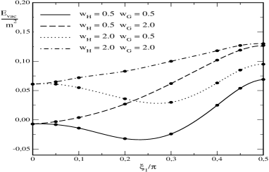
Except for narrow string configurations dominated by the Higgs field, the vacuum polarization energy turns out to be positive. Therefore, fermionic vacuum fluctuations alone do not provide any substantial binding and no stable uncharged string is found for the physically motivated parameters, eq. (8), for which $E_{\rm cl}$ dominates the total energy. Since $E_{\rm cl}$ decreases quickly with increasing Yukawa coupling $f$, some stability is indeed seen for large $f$ and narrow strings but in this regime the restriction to one fermion loop in the vacuum polarization energy is unreliable because of the unphysical Landau ghost contribution Ripka:1987ne ; Hartmann:1994ai .

V Charged Strings

Cosmic strings induce many fermionic bound state levels for the two–dimensional scattering problem, whose energies are denoted by $\epsilon_{j}$. For $\xi_{1}=\xi_{2}=\pi/2$ there even exists an exact zero modeNaculich:1995cb . In the three–dimensional setting these bound states acquire a longitudinal momentum for the motion along the symmetry axis, i.e. their energies become

$$E_{i}(p_{n})=\sqrt{\epsilon_{i}^{2}+p_{n}^{2}}\qquad{\rm with}\qquad p_{n}=\frac{n\pi}{L}\,.$$ (27)

Here $L$ is the length of the string. To leading order of the limit $L\to\infty$, the sum over the discrete longitudinal momentum turns into a continuum integral, $\sum_{n}\,\longrightarrow\,\frac{L}{\pi}\int_{0}^{\infty}dp$. To find the minimal bound state contribution at a fixed charge (per unit length), a chemical potential $\mu$ with ${\rm max}(|\epsilon_{j}|)\leq\mu\leq m$ is introduced, and all levels with $E_{i}(p)\leq\mu$ are populated. This procedure defines a Fermi momentum for each level, $p^{F}_{i}(\mu)\equiv\sqrt{\mu^{2}-\epsilon_{i}^{2}}$ which enters the total charge per unit length of the string

$$Q(\mu)=\sum_{i}\frac{p^{F}_{i}(\mu)}{\pi}\,.$$ (28)

This relation can be inverted to give $\mu=\mu(Q)$ and thus $p^{F}_{i}=p^{F}_{i}(Q)$. This quantity provides, for a given charge $Q$, the maximal momentum along the string direction for each fermion to get trapped in a two-dimensional bound state $\epsilon_{i}$ perpendicular to the string. From this the binding energy (per unit length) for a prescribed charge

$$E_{\rm bind}(Q)=\frac{1}{\pi}\sum_{i}\int_{0}^{p^{F}_{i}(Q)}dp\,\left[\sqrt{\epsilon_{i}^{2}+p^{2}}-m\right]$$ (29)

is computed relative to an equal number of free fermions that have energy $m$ each.

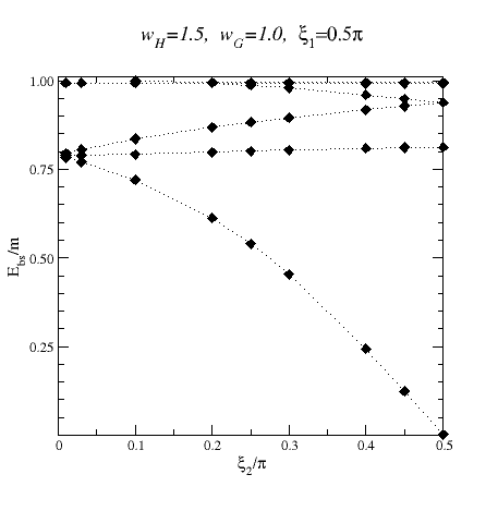
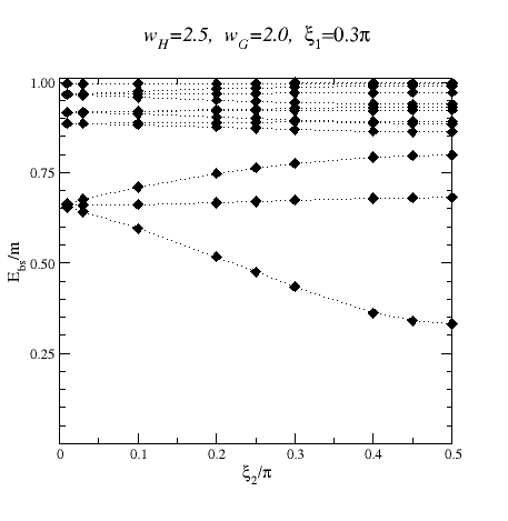
Figure 2 shows the fermion contribution to the binding energy, $E_{\rm vac}+E_{\rm bind}(Q)$. In the left panel the graph terminates for a given configuration when all available bound state levels are occupied and the charge cannot be increased any further. For small charges, narrow strings are favorable while the binding energy of wider strings decreases more quickly as $Q$ increases.

         

Figure 2: (Color online) Fermion contribution to the energy of a charged string (left panel). Total energy of the charged string (right panel) as function of the charge density.

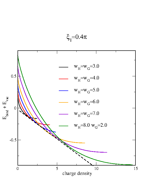
Surprisingly, the envelope along which $E_{\rm vac}+E_{\rm bind}$ is minimal (when varying the string parameters at fixed charge) forms a straight line. Extrapolating this line to  $Q=0$  indicates that the fermion vacuum polarization energy should (approximately) vanish. This extrapolation circumvents the Landau ghost problem mentioned in the previous section.

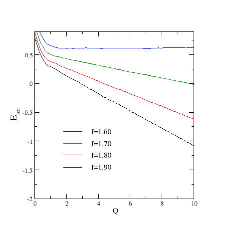
To finally decide on dynamical stability, the classical energy must be included as well. To this end several hundred configurations, that are characterized by the variational ansätze, eq. (25), were scanned. It is appropriate to label them by $s=1,2,\dots$ and to compute their total binding energy as

$$E^{(s)}_{\rm tot}(Q)=E^{(s)}_{\rm cl}+N_{C}\left[E^{(s)}_{\rm vac}+E^{(s)}_{\rm bind}(Q)\right]$$ (30)

for a given charge. If

$$E_{\rm tot}(Q)\equiv{\rm min}_{s}\left[E^{(s)}_{\rm tot}(Q)\right]<0$$ (31)

a stable configuration has been found. The right panel of figure  2 shows $E_{\rm tot}$ as a function of charge for various values of the Yukawa coupling constant. Since the mass $m$ of a non–interacting fermion sets the scale in the numerical analysis, this refers to different values of the dimensionless ratio $v/m$. For $f\approx 1.6$ the classical and fermion energies essentially cancel each other and leave $E_{\rm tot}$ roughly independent of charge. Bound objects are observed by further increasing the Yukawa coupling to about $f\approx 1.7$, which corresponds to a heavy fermion mass which is still less than twice the top quark mass. The minimizing configurations have $\xi_{1}\approx 0$, i.e. they are dominated by the Higgs field. The numerical results reviewed here largely support the existence of a novel solution within the standard model of particle physics. These string configurations exist provided that a sufficient density of very heavy fermions is present which can be trapped to the string core to stabilize the configuration. Such conditions may have existed in the early universe, and the emerging cosmic strings should still be traceable today. Inverting this argument, not observing cosmic strings indicates that fermions coupling to the weak interactions in the usual way cannot have existed with sufficient density if their mass exceeds about twice the top–quark mass, unless they can decay to lighter fermions.

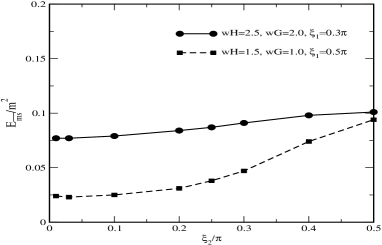
VI Variational parameter $\mathbf{\xi_{2}}$

So far the numerical analysis of the charged string was limited to the case of $\xi_{2}=\pi/2$, for which the scattering and bound state problems only involve real valued Hamiltonians. First numerical results for the vacuum polarization energy at $\xi_{2}\neq\pi/2$ are shown in the right panel of figure 1. They suggest that reducing $\xi_{2}$ may indeed further decrease the vacuum polarization energy. However, the contribution from explicitly occupying the bound fermion levels may have the opposite effect. The numerical determination of the bound state energies is more complicated when the Hamiltonian is not real. Rather than doubling the diagonalization problem by separating real and imaginary parts, it is easier to extract the bound state energies from the roots of the Jost function at complex momentum. Since this Jost function results from a multi–channel problem, its roots need not be simple which adds to the difficulty of extracting them numerically. Fortunately, Levinson’s theorem Levinson:1949 ; Puff:1975zz yields the number of expected bound states from the phase shifts. The typical behavior of the bound state energies as a function of $\xi_{2}$ is shown in figure 3. Note that the zero mode for $\xi_{1}=\frac{\pi}{2}$ and $\xi_{2}=\frac{\pi}{2}$ is recovered. Similarly to decreasing $\xi_{1}$, any reduction of $\xi_{2}$ also reduces the binding of that level.

             

Figure 3: The variation of the zero modes as a function of $\xi_{2}$ for narrow (left panel) and wide (right panel) string profiles. The dots indicate calculated values while the lines have been added to guide the eye.

The data from the $\xi_{2}$-variation can only lower the minimal total energy which further reduces the bound on $f$ and thus the mass of the trapped fermion below which a charged cosmic string is stable. The conclusions made at the end of the previous section remain valid, but the bounds and statements become more stringent.

VII Closed Nielsen–Olesen Strings

Cosmic strings usually carry magnetic flux and are thus particle analogs of Abrikosov vortices in type-II superconductors. Since the flux is conserved, the vortex must either end on (magnetic) charges or be closed. The preferred topology of strings formed during the electroweak phase transition are thus closed rings which may be stabilized dynamically – either by spinning at high angular momenta Witten:1984eb , by extra currents running along the ring Witten:1984eb ; Davis , or by trapping charged particles as discussed earlier. Such stable vortex configurations are called vortons Davis:1988ij .

If none of these stabilizing effects is operative, the vorton will follow its (classical) instability and collapse by radiating away its energy. Again, this picture may be altered by quantum fluctuations: Due to the uncertainty principle, there is a quantum mechanical penalty for localizing in a very small volume. This quantum energy may ultimately balance the classical energy of the vorton and stabilize it at some small radius.

The size of such quantum stabilized vortons is expected to be of the order of the Compton wavelength of the fluctuating field – not the astrophysical scales over which the initial string stretched. Nonetheless, vortons are expected to be produced during the electroweak phase transition at such high rates that they would naturally evolve into acceptable densities of (neutral) dark matter Davis:1988ij . There are also stringent experimental constraints on the density of charged dark matter Fukugita:1990uh and thus charged vortons, which may help to rule out certain cosmology models that produce such vortons copiously.

In this section, we investigate a quantum mechanism to stabilize neutral close Nielsen–Olesen type of vortices against collapsing to zero radius. The model is that of scalar electrodynamics with the Lagrangian as in eq. (5), but with both the Higgs and the gauge fields now $U(1)$ valued. The fields of the Nielsen–Olesen string along the infinitely long symmetry axis are similar to those in eqs. (1) and (2) with the $2\times 2$ matrices replaced by the identity matrix. They are transformed to closed strings by taking the symmetry axis to be of finite length, say $2\pi R$, and then connecting the end points. The symmetry axis thus turns into a circle along which the core of the string is located. When this circle is embedded in the $x$–$y$ plane and centered in the origin, it is appropriate to introduce toroidal coordinates book_MF as

$$x=R\,\frac{\sinh\tau\cos\varphi}{\cosh\tau-\cos\sigma}\,,\qquad y=R\,\frac{\sinh\tau\sin\varphi}{\cosh\tau-\cos\sigma}\,,\qquad z=R\,\frac{\sin\sigma}{\cosh\tau-\cos\sigma}\,.$$ (32)

The angle $\varphi\in[0,2\pi]$ parameterizes the symmetry transformation along the core circle, i.e. the profiles will not depend on this variable. For a constant angle $\varphi$, the lines of constant $\tau\in[0,\infty]$ are circles that enclose the core of the string. Smaller values of $\tau$ correspond to larger circles that spread out towards infinity on the outside, and approach the $z$–axis on the inside. The inverse $1/\tau$ is therefore (in a highly non–linear fashion) related to the distance from the string core, similarly to the radius $\rho$ in the linear Nielsen–Olesen string. Finally, the angle $\sigma\in[0,2\pi]$ parameterizes the points on the fixed $\tau$-circles enclosing the string core, i.e. it acts like an azimuthal angle when viewed from the core circle. It is therefore natural to give the Higgs field winding by taking $\sigma$ as its phase. Then the profiles are predominantly functions of $\tau$ only, independent of $\varphi$, with (probably moderate) modulation in $\sigma$, mainly in the vicinity of the origin. The origin corresponds to $\tau=0$ and $\sigma=\pi$, while spatial infinity is approached as $\tau\to 0$ and $\sigma\to 0$.

Note that the $\sigma$–modulation, even if it turns out to be fairly small, cannot be avoided all together: For fixed $\varphi$ and $\tau=0$, $\sigma=0\ldots\pi$ parameterizes the positive $z$–axis. At each point along this axis the core of the string is seen with a different opening angle. For $\tau>0$ but $\tau\ll 1$, varying $\sigma$ corresponds to moving along a circle enclosing the string core. One side of this circle corresponds to the far distance, while the other side is close to the origin. Obviously, different $\sigma$ values refer to distinct phyiscal regions and the fields must hence depend on this angle. In contrast to the linear Nielsen–Olesen string, the profile functions must hence depend on two coordinates, which complicates matters significantly. To be explicit, an appropriate ansatz is

$$\Phi=vf(\sigma,\tau)\,{\rm e}^{in\sigma}\qquad{\rm and}\qquad\mbox{\boldmath$A$\unboldmath}=\frac{n}{eR}\,\eta(\sigma,\tau)\,g(\sigma,\tau)\mbox{\boldmath$e$\unboldmath}_{\sigma}\,.$$ (33)

The metric factor $\eta=\cosh\tau-\cos\sigma$, as well as the inverse coupling constant and radius, have been introduced to ensure that $f\equiv 1$ and $g\equiv 1$ correspond to a pure gauge configuration. Recall that the profiles $f$ and $g$ depend on the choice of the dimensionless radius $\hat{R}\equiv m_{W}R$. With these preliminaries the classical energy becomes

$$\frac{E}{m_{W}}=\frac{\pi}{g^{2}}\int_{0}^{\infty}d\tau\int_{-\pi}^{\pi}d\sigma\,\sinh\tau\,\Bigg{\{}\frac{n^{2}}{\hat{R}\eta}\,(\partial_{\tau}g)^{2}+\hat{R}\eta\,\Big{[}(\partial_{\tau}f)^{2}+n^{2}f^{2}\,\big{(}1-g\big{)}^{2}+(\partial_{\sigma}f)^{2}\Big{]}+\frac{m_{\Phi}^{2}}{4m_{W}^{2}}\,\hat{R}^{3}\,\eta^{3}\,\big{(}1-f^{2}\big{)}^{2}\Bigg{\}}\,,$$ (34)

subject to the boundary conditions

$$f(0,\tau)=f(2\pi,\tau)\,,\qquad g(0,\tau)=g(2\pi,\tau)\,,\qquad{\rm and}\qquad f(\sigma,\infty)=g(\sigma,\infty)=0\,.$$ (35)

Furthermore, Neumann boundary conditions for $\sigma\neq 0,2\pi$,

$$\partial_{\tau}f(\sigma,0)=\partial_{\tau}g(\sigma,0)=0\,,$$ (36)

ensures that any solution of the field equations with finite total energy will approach $f=g=1$ as $\sigma\to 0$ or $\sigma\to 2\pi$ when $\tau=0$.

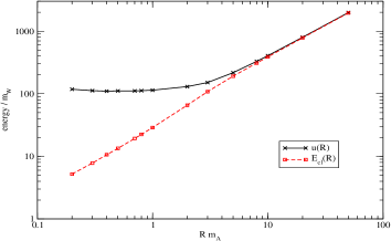
A detailed description of the relaxation method for constructing the actual field configuration numerically constrained to a prescribed value of the radius parameter $\hat{R}$ can be found in ref. Quandt:2013qxa . Here we just review the results for the minimal energy in figure 4.

                 

Figure 4: The classical energy (left panel) and the energy per unit length of the core circle (right panel) for a closed Nielsen–Olesen string as functions of the core radius. The stars indicate the numerically computed cases. Data are presented for $g=1/\sqrt{2}$ and $m_{\Phi}=m_{W}$, for which the straight string has energy per unit length $6.28\,m_{W}^{2}$.

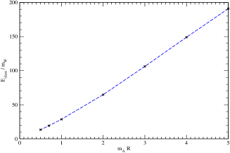
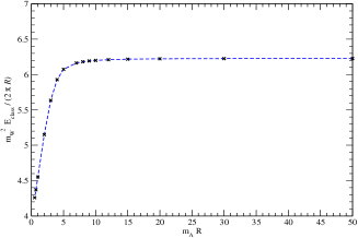
The left panel essentially reveals an almost linear relation between the minimal energy and the radius. More interesting is the energy per length of the torus, which is shown in the right panel. The first observation is a saturation at large radii. This is nothing but the energy per unit length of the infinitely long string, i.e. the Nielson-Olesen limit. Reproducing this known result is a strong consistency check of our numerical treatment. Interestingly, the saturation occurs already for radii only slightly larger than the Compton wave–length of the gauge field. This suggests that energy loss from radiating gauge and/or Higgs fluctuations is indeed irrelevant for simulations of networks of closed strings that refer to cosmological length scales. For smaller radii, the interaction between opposite sides of the torus leads to a considerable drop in the energy per unit length. As a consequence, the total energy of the torus configuration decays more than linearly at small core radii $R\to 0$, which means that it is classically unstable against shrinking to a point. Of course, this instability is expected from Derrick’s theorem, according to which higher order derivative terms (as in the Skyrme modelSkyrme:1961vq ) would be needed to stabilize a localized object in three space dimensions.

Of course, quantum mechanically such an instability could represent a violation of Heisenberg’s uncertainty principle according to which field configurations localized within an arbitrarily small region must have large energy and/or momentum. To investigate this question, we elevate the radius to quantum variable and treat it as a collective coordinate. In a first step we take $R=R(t)$ to be time dependent and then identify its conjugate momentum. Since the Cartesian coordinates are fixed in terms of $R$, this implements a time dependence of the fields via eq. (32). Once $A$ is time dependent, its temporal component can no longer vanish but will be induced via Gauß’ law. As a result, it will be proportional to the time derivative $\dot{R}=\frac{dR(t)}{dt}$. Thus the Gauß’ law augments the field configuration by the additional profile function $q$ via

$$e\,A_{0}(\mathbf{x},t)=\frac{\dot{R}}{R}\,q(\sigma,\tau)\,.$$ (37)

Putting things together yields the action functional for the unstable mode

$$S=\int dt\,\left[\frac{1}{2}\,u(R)\,\dot{R}^{2}-E(R)\right]\,.$$ (38)

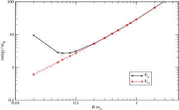
The energy functional $E(R)$ is that of eq. (34) while the explicit expression for the mass functional $u(R)$ is fairly complicated and given in detail in ref. Quandt:2013qxa . Here it suffices to mention that $u(R)$ contains linear and quadratic terms in the induced profile $q$. The profile functions $f$ and $g$ are determined from minimizing $E(R)$. In turn they provide source terms for $q$ when applying the variational principle to $u(R)$. This procedure is equivalent to solving the Gauß law constraint Quandt:2013qxa . The resulting mass functional is shown in the left panel of figure 5 as a function of the radius $R$.

The action functional, eq. (38) yields the canonical momentum (operator) $p$ and, via Legernde transformation, the (quantum) energy of the unstable mode as

$$p=u(R)\frac{dR}{dt}\qquad{\rm and}\qquad E=\frac{p^{2}}{2u(R)}+E(R)\,.$$ (39)

Figure 5 shows that $u(R)$ is huge for radii larger than the Compton wave–length of the gauge boson. For a fixed momentum, the back–reaction of the classical profiles $f$ and $g$ due to the induced kinetic term in eq. (39) is of the order $\mathcal{O}(u^{-2})$. This effect can thus be safely omitted and these profile functions are reliably obtained by applying the variational principle to $E(R)$ alone. As mentioned earlier, $q$ is subsequently obtained from varying $u(R)$, and, since initial profiles $f$ and $g$ need not be re-computed, the parameter functions in eq. (39) are then completely determined. The corresponding Hamilton operator can then be constructed by imposing canonical commutation relations for $p$ and $R$. The ground state (g.s.) energy eigenvalue can easily be estimated by recalling that the uncertainty principle establishes its lower bound in the form

$$E_{\rm g.s.}\geq\frac{\hbar^{2}}{2u(R)R^{2}}+E(R)\,.$$ (40)

This total energy of the torus string is displayed as a function of $R$ in the right panel of figure 5. Obviously a local minimum at non–zero torus radius $R$ exists, suggesting the quantum stabilization of the closed Nielsen–Olesen string. As for the infinitely long charged string, the length scale at which stability occurs is quite small and it is unclear whether it leads to significant cosmological implications.

             

Figure 5: The mass functional for the unstable mode (left panel) and the lower boundary for its quantum energy (right panel). Also shown are the classical energies.

VIII Conclusion

This review has mainly focused on computing the fermion contribution to the vacuum polarization energy per unit length of an infinitely long straight string in a simplified version of the electroweak standard model. The approach is based on the interface formalism, for which the analytical properties of scattering data are essential. Obstacles that arise in a naïve treatment from the non–trivial structure of the string configuration at spatial infinity are circumvented by choosing a particular subset of gauges. Numerically the vacuum polarization turns out to be small and positive in the regime in which the one–fermion loop approximation is reliable. Hence, there is no quantum stabilization of the (uncharged) string. However, it also turns out that a heavy fermion doublet can stabilize a non–trivial string background if such fermions are trapped at the string core to give it a non–zero fixed charge per unit length. The resulting configuration is dominated by the Higgs field. Since any additional variational degree of freedom can only lower the total energy, the embedding of this configuration in the full standard model, with the $U(1)$ gauge field included, will also yield a bound object, at least if the mixing between this heavy fermion and the known standard model fermions can be ignored. Numerically binding sets in at $m\approx 300\,\mathrm{GeV}$, which is still within the range of energy scales at which the standard model is expected to provide an effective description of the relevant physics, and also within the range to be probed at the LHC. Light fermions would contribute only weakly to the binding of the string, since their Yukawa couplings are small. We emphasize that this cosmic string configuration is a novel solution in a model that is very closely related to the standard model of particle physics. At a similar scale, though through a different mechanism, quantum effects may also prevent neutral closed strings from collapsing.

References

- (1) T. Vachaspati, Phys. Rev. Lett. 68, 1977 (1992) [Erratum-ibid. 69, 216 (1992)].
- (2) A. Achucarro and T. Vachaspati, Phys. Rept. 327, 347 (2000).
- (3) Y. Nambu, Nucl. Phys. B 130, 505 (1977).
- (4) H. B. Nielsen and P. Olesen, Nucl. Phys. B 61, 45 (1973).
- (5) A. Achucarro and C. J. A. Martins, arXiv:0811.1277 [astro-ph].
- (6) E. J. Copeland and T. W. B. Kibble, Proc. Roy. Soc. Lond. A 466, 623 (2010).
- (7) R.H. Brandenberger and A. Davis, Phys. Lett. B 308, 79 (1993);
- (8) R.H. Brandenberger, A. Davis, and M. Trodden, Phys. Lett. B 335, 123 (1994).
- (9) K. Kajantie, M. Laine, K. Rummukainen, and M. E. Shaposhnikov, Phys. Rev. Lett. 77 , 2887 (1996); K. Rummukainen, M. Tsypin, K. Kajantie, M. Laine, and M. E. Shaposhnikov, Nucl. Phys. B 532 , 283 (1998); F. Csikor, Z. Fodor, and J. Heitger, Phys. Rev. Lett. 82 , 21 (1999).
- (10) C. Grojean, G. Servant, and J. D. Wells, Phys. Rev. D 71, 036001 (2005); A. Menon, D. E. Morrissey, and C. E. M. Wagner, Phys. Rev. D 70, 035005 (2004).
- (11) A. Vilenkin, Phys. Rept. 121, 263 (1985).
- (12) M. B. Hindmarsh and T. W. B. Kibble, Rept. Prog. Phys. 58, 477 (1995).
- (13) R. H. Brandenberger, Int. J. Mod. Phys. A 9, 2117 (1994).
- (14) A. Albrecht and N. Turok, Phys. Rev. D 40, 973 (1989).
- (15) E. D’Hoker and E. Farhi, Nucl. Phys. B 248, 59 (1984); 77 (1984).
- (16) S. G. Naculich, Phys. Rev. Lett. 75, 998 (1995).
- (17) F. R. Klinkhamer and C. Rupp, J. Math. Phys. 44, 3619 (2003).
- (18) G. Starkman, D. Stojkovic, and T. Vachaspati, Phys. Rev. D 65, 065003 (2002); G. Starkman, D. Stojkovic, and T. Vachaspati, Phys. Rev. D 63, 085011 (2001); D. Stojkovic, Int. J. Mod. Phys. A 16S1C, 1034 (2001).
- (19) M. Groves and W. B. Perkins, Nucl. Phys. B 573, 449 (2000).
- (20) M. Bordag and I. Drozdov, Phys. Rev. D 68, 065026 (2003).
- (21) J. Baacke and N. Kevlishvili, Phys. Rev. D 78, 085008 (2008).
- (22) M. Lilley, F. Di Marco, J. Martin, and P. Peter, Phys. Rev. D 82, 023510 (2010).
- (23) H. Weigel, M. Quandt, N. Graham, and O. Schröder, Nucl. Phys. B 831, 306 (2010).
- (24) H. Weigel and M. Quandt, Phys. Lett. B 690, 514 (2010).
- (25) H. Weigel, M. Quandt, and N. Graham, Phys. Rev. Lett. 106, 101601 (2011).
- (26) N. Graham, M. Quandt, and H. Weigel, Phys. Rev. D 84, 025017 (2011).
- (27) G. H. Derrick J. Math. Phys. 5, 1252 (1964).
- (28) M. Quandt, N. Graham, and H. Weigel, Phys. Rev. D 87, 085013 (2013).
- (29) N. Graham, M. Quandt, O. Schroeder, and H. Weigel, Nucl. Phys. B 758, 112 (2006).
- (30) N. Graham, M. Quandt, and H. Weigel, Lect. Notes Phys. 777, 1 (2009).
- (31) N. Graham, R. L. Jaffe, M. Quandt, and H. Weigel, Phys. Rev. Lett. 87, 131601 (2001).
- (32) M. G. Krein, Mat. Sborn. (N.S.) 33, 597 (1953); M. G. Krein, Sov. Math.–Dokl. 3, 707 (1962); M. Sh. Birman and M. G. Krein, Sov. Math.–Dokl. 3, 740 (1962).
- (33) N. Graham, R. L. Jaffe, V. Khemani, M. Quandt, M. Scandurra, and H. Weigel, Nucl. Phys. B 645, 49 (2002).
- (34) R. D. Puff, Phys. Rev. A 11, 154 (1975); N. Graham, R. L. Jaffe, M. Quandt, and H. Weigel, Annals Phys. 293, 240 (2001).
- (35) N. Levinson, Kgl. Dansk Videskab Selskab, Mat-fys. Medd. 25 (1949) 9; G. Barton, J. Phys. A18, 479 (1985).
- (36) N. Graham, V. Khemani, M. Quandt, O. Schröder, and H. Weigel, Nucl. Phys. B 707, 233 (2005); H. Weigel, J. Phys. A 39, 6799 (2006).
- (37) P. M. Morse and H. Feshbach, Methods in Theoretical Physics, chapter 5, McGraw-Hill 1953.
- (38) E. Farhi, N. Graham, R. L. Jaffe, and H. Weigel, Nucl. Phys. B 630, 241 (2002).
- (39) G. Ripka and S. Kahana, Phys. Rev. D 36, 1233 (1987).
- (40) J. Hartmann, F. Beck, and W. Bentz, Phys. Rev. C 50, 3088 (1994).
- (41) E. Witten, Nucl. Phys. B 249, 557 (1985).
- (42) A. C. Davis and P. Peter, Phys. Lett. B 358, 197 (1995); A. C. Davis and W. B. Perkins, Phys. Lett. B 390, 107 (1997); S. C. Davis, W. B. Perkins, and A. C. Davis, Phys. Rev. D 62, 043503 (2000).
- (43) R. L. Davis and E. P. S. Shellard, Nucl. Phys. B 323, 209 (1989).
- (44) M. Fukugita, P. Hut, and N. Spergel, IASSNS-AST-88-26 (1990).
- (45) T. H. R. Skyrme, Proc. Roy. Soc. Lond. A 260, 127 (1961); G. S. Adkins, C. R. Nappi, and E. Witten, Nucl. Phys. B 228, 552 (1983); H. Weigel, Lect. Notes Phys. 743, 1 (2008).