High-order compact schemes for Black-Scholes basket options

Abstract

We present a new high-order compact scheme for the multi-dimensional Black-Scholes model with application to European Put options on a basket of two underlying assets. The scheme is second-order accurate in time and fourth-order accurate in space. Numerical examples confirm that a standard second-order finite difference scheme is significantly outperformed.

1 Introduction

The multidimensional Black-Scholes model for option pricing (e.g. [8]) considers $n\in\mathbb{N}_{\geq 2}$ underlying assets $S_{i}\in[0,\infty[$ for $i=1,\ldots,n$, where each asset follows a geometric Brownian motion,

$${\rm d}S_{i}(t) =\mu_{i}S_{i}(t){\rm d}t+\sigma_{i}S_{i}(t){\rm d}W^{(i)}(t),$$ (1)

where $\mu_{i}\in\mathbb{R}$ is the drift and $\sigma_{i}\geq 0$ is the volatility of the asset $S_{i}$, respectively, for $i=1,\ldots,n$ and ${\rm d}W^{(i)}(t)$ denotes a Wiener Process at time $t\in[0,T]$ for some $T>0$. The correlation between the assets is given by ${\rm d}W^{(i)}(t){\rm d}W^{(j)}(t)=\rho_{ij}{\rm d}t$. The Lemma of Itô and standard no-arbitrage arguments lead to the following (backward in time) parabolic partial differential equation with mixed second-order derivative terms for the option price $V=V(S_{1},S_{2},\dots,S_{n},t)$ (see, e.g. [8]),

$$\frac{\partial V}{\partial t}+\frac{1}{2}\sum\limits_{i=1}^{n}\sigma_{i}^{2}S_{i}^{2}\frac{\partial^{2}V}{\partial S_{i}^{2}}+\sum\limits_{\begin{subarray}{c}i,j=1\\ i<j\end{subarray}}^{n}\rho_{ij}\sigma_{i}\sigma_{j}S_{i}S_{j}\frac{\partial^{2}V}{\partial S_{i}\partial S_{j}}+\sum\limits_{i=1}^{n}rS_{i}\frac{\partial V}{\partial S_{i}}-rV= 0,$$

with $S_{i}>0$, $t\in[0,T[$ and $r\geq 0$ denoting the riskless interest rate. When examining a European Put basket option, the final condition is given by

$$V(S_{1},\ldots,S_{n},T)= \max\biggl{(}K-\sum\limits_{i=1}^{n}\omega_{i}S_{i},0\biggr{)},$$

where the asset weights satisfy $\sum\limits_{i=1}^{n}\omega_{i}=1$ and additionally $\omega_{i}>0$ for $i=1,\ldots,n$ if we have short-selling restrictions. Suitable boundary conditions are discussed later.

The transformations

$$x_{i}= \frac{\gamma}{\sigma_{i}}\ln\left(\frac{S_{i}}{K}\right),\quad\tau=T-t\quad\text{ and }\quad u=e^{r\tau}\frac{V}{K},$$ (2)

where $\gamma>0$ is a constant scaling parameter, yield the (forward in time) parabolic partial differential equation

$$u_{\tau}-\frac{\gamma^{2}}{2}\sum\limits_{i=1}^{n}\frac{\partial^{2}u}{\partial x_{i}^{2}}-\gamma^{2}\sum\limits_{\begin{subarray}{c}i,j=1\\ i<j\end{subarray}}^{n}\rho_{ij}\frac{\partial^{2}u}{\partial x_{i}\partial x_{j}}+\gamma\sum\limits_{i=1}^{n}\left[\frac{\sigma_{i}}{2}-\frac{r}{\sigma_{i}}\right]\frac{\partial u}{\partial x_{i}}= 0,$$ (3)

where $x\in\mathbb{R}^{n}$ and $\tau\in\Omega_{\tau}=]0,T]$. Under the same transformations the initial condition for a European Put basket is given by

$$u(x_{1},\ldots,x_{n},0)= \max\biggl{(}1-\sum\limits_{i=1}^{n}\omega_{i}e^{\frac{\sigma_{i}x_{i}}{\gamma}},0\biggr{)}.$$ (4)

When looking for numerical methods to approximate solutions to problem (3), (4), subject to suitable boundary conditions, finite difference schemes can be employed, at least for space dimensions up to three. Standard discretisations, however, only yield second-order convergence in terms of the spatial discretisation parameter. Alternatively, high-order compact schemes can be used which only use points on a compact computational stencil, while having fourth-order consistency in space, see for example [4, 6, 7, 1, 2] and the references therein. A drawback is that the derivation of high-order compact schemes (and their numerical stability analysis) is algebraically demanding, hence most works in this area restrict themselves to the one-dimensional case. An additional complication is present in (3) in form of the mixed second-order derivative terms.

In a forthcoming paper [3] we derive new high-order compact schemes for a rather general class of linear parabolic partial differential equations with mixed second-order derivative terms and time- and space-dependent coefficients in arbitrary space dimension $n\in\mathbb{N}$. In the present paper we focus on the multi-dimensional Black-Scholes model (3), (4). We present a new high-order compact scheme which is second-order accurate in time and fourth-order accurate in space. To ensure high-order convergence in the presence of the initial condition (4) with low regularity we employ the smoothing operators of Kreiss et al. [5]. Numerical examples for pricing European Put options on a basket of two underlying assets confirm that a standard second-order finite difference scheme is significantly outperformed.

2 Discrete two-dimensional Black-Scholes equation

For the discretisation of (3) with $n=2$ we replace the spatial domain by the rectangle $\Omega=[x_{\min}^{(1)},x_{\min}^{(1)}]\times[x_{\min}^{(2)},x_{\min}^{(2)}]$ with $-\infty<x_{\min}^{(i)}<x_{\min}^{(i)}<\infty$ for $i=1,2$. On $\Omega$, we define the grid

$$G^{(2)}_{h}=\big{\{}(x^{(1)}_{i_{1}},x^{(2)}_{i_{2}})\in\Omega\text{ }|\text{ }x^{(k)}_{i_{k}}=x_{\min}^{(k)}+i_{k}h,\,1\leq i_{k}\leq N_{k},\,k=1,2\big{\}},$$ (5)

where $h>0$, $N_{k}\in\mathbb{N}$ and $x_{\max}^{(k)}=x_{\min}^{(k)}+N_{k}h$ for $k=1,2$. By $\overset{\smash{\raisebox{-0.51663pt}{$\scriptstyle\circ$}}}{G}\rule{0.0pt}{9.90276pt}^{(2)}_{h}$ we denote the interior of $G^{(2)}_{h}$. We present the coefficients of a semi-discrete scheme of the form

$$\sum\limits_{j_{1}=i_{1}-1}^{i_{1}+1}\sum\limits_{j_{2}=i_{2}-1}^{i_{2}+1}\left[\hat{M}_{j_{1},j_{2}}\partial_{\tau}U_{j_{1},j_{2}}(\tau)+\hat{K}_{j_{1},j_{2}}U_{j_{1},j_{2}}(\tau)\right]= \tilde{g}(x,\tau),$$

at time $\tau$ for each point $x\in\overset{\smash{\raisebox{-0.51663pt}{$\scriptstyle\circ$}}}{G}\rule{0.0pt}{9.90276pt}_{h}^{(2)}$ for the two-dimensional Black-Scholes equation using $n=2$ in (3). By $U_{j_{1},j_{2}}(\tau)$ we denote the approximation of $u(x_{i_{1}}^{(1)},x_{i_{2}}^{(2)},\tau)$ after semi-discretisation in space with $\bigl{(}x_{i_{1}}^{(1)},x_{i_{2}}^{(2)}\bigr{)}\in G_{h}^{(2)}$.

The general idea underlying the derivation of the high-order compact scheme is to operate on the differential equation (3) as an additional relation to obtain finite difference approximations for high-order derivatives in the truncation error. Inclusion of these expressions in a central difference method for equation (3) increases the order of accuracy to fourth order while retaining a compact stencil. A detailed derivation of this scheme and a thorough von Neumann stability analysis are presented in a forthcoming paper [3]. In the two-dimensional case we obtain the following coefficients

$$\hat{K}_{i_{1},i_{2}}= -\,{\frac{2{\gamma}^{2}{\rho^{2}_{{12}}}}{3{h}^{2}}}+\,{\frac{5{\gamma}^{2}}{3{h}^{2}}}+\frac{\left(\frac{\sigma_{{1}}}{2}-{\frac{r}{\sigma_{{1}}}}\right)^{2}}{3}+\frac{\left(\frac{\sigma_{{2}}}{2}-{\frac{r}{\sigma_{{2}}}}\right)^{2}}{3},$$

$$\hat{K}_{i_{1}\pm 1,i_{2}}= \,{\frac{{\gamma}^{2}{\rho^{2}_{{12}}}}{3{h}^{2}}}\pm\frac{\gamma\,\left(\frac{\sigma_{{1}}}{2}-{\frac{r}{\sigma_{{1}}}}\right)}{3h}\mp\frac{\gamma\,\left(\frac{\sigma_{{2}}}{2}-{\frac{r}{\sigma_{{2}}}}\right)\rho_{{12}}}{3h}-\frac{\left(\frac{\sigma_{{1}}}{2}-{\frac{r}{\sigma_{{1}}}}\right)^{2}}{6}-\,{\frac{{\gamma}^{2}}{3{h}^{2}}},$$

$$\hat{K}_{i_{1},i_{2}\pm 1}= \,{\frac{{\gamma}^{2}{\rho^{2}_{{12}}}}{3{h}^{2}}}\pm\frac{\gamma\,\left(\frac{\sigma_{{2}}}{2}-{\frac{r}{\sigma_{{2}}}}\right)}{3h}\mp\frac{\gamma\left(\frac{\sigma_{{1}}}{2}-{\frac{r}{\sigma_{{1}}}}\right)\,\rho_{{12}}}{3h}-\frac{\left(\frac{\sigma_{{2}}}{2}-{\frac{r}{\sigma_{{2}}}}\right)^{2}}{6}-\,{\frac{{\gamma}^{2}}{3{h}^{2}}},$$

$$\hat{K}_{i_{1}\pm 1,i_{2}-1}= \pm\frac{\left(\frac{\sigma_{{2}}}{2}-{\frac{r}{\sigma_{{2}}}}\right)\left(\frac{\sigma_{{1}}}{2}-{\frac{r}{\sigma_{{1}}}}\right)}{12}-\frac{\gamma\,\left(\frac{\sigma_{{2}}}{2}-{\frac{r}{\sigma_{{2}}}}\right)}{12h}\pm\frac{\gamma\,\left(\frac{\sigma_{{1}}}{2}-{\frac{r}{\sigma_{{1}}}}\right)}{12h}$$

$$-\frac{\gamma\left(\frac{\sigma_{{1}}}{2}-{\frac{r}{\sigma_{{1}}}}\right)\,\rho_{{12}}}{6h}\pm\frac{\gamma\,\left(\frac{\sigma_{{2}}}{2}-{\frac{r}{\sigma_{{2}}}}\right)\rho_{{12}}}{6h}-\,{\frac{{\gamma}^{2}}{12{h}^{2}}}\pm\,{\frac{{\gamma}^{2}\rho_{{12}}}{4{h}^{2}}}-\,{\frac{{\gamma}^{2}{\rho^{2}_{{12}}}}{6{h}^{2}}},$$

$$\hat{K}_{i_{1}\pm 1,i_{2}+1}= \frac{\gamma\,\left(\frac{\sigma_{{2}}}{2}-{\frac{r}{\sigma_{{2}}}}\right)}{12h}\mp\frac{\left(\frac{\sigma_{{2}}}{2}-{\frac{r}{\sigma_{{2}}}}\right)\left(\frac{\sigma_{{1}}}{2}-{\frac{r}{\sigma_{{1}}}}\right)}{12}\pm\frac{\gamma\,\left(\frac{\sigma_{{1}}}{2}-{\frac{r}{\sigma_{{1}}}}\right)}{12h}$$

$$+\frac{\gamma\,\rho_{{12}}\left(\frac{\sigma_{{1}}}{2}-{\frac{r}{\sigma_{{1}}}}\right)}{6h}\pm\frac{\gamma\,\left(\frac{\sigma_{{2}}}{2}-{\frac{r}{\sigma_{{2}}}}\right)\rho_{{12}}}{6h}-\,{\frac{{\gamma}^{2}}{12{h}^{2}}}\mp\,{\frac{{\gamma}^{2}\rho_{{12}}}{4{h}^{2}}}-\,{\frac{{\gamma}^{2}{\rho^{2}_{{12}}}}{6{h}^{2}}},$$

as well as

$$M_{i_{1}+1,i_{2}\pm 1}= M_{i_{1}-1,i_{2}\mp 1}=\pm\frac{\rho_{{12}}}{24}, M_{i_{1},i_{2}}= \frac{2}{3},$$

$$M_{i_{1}\pm 1,i_{2}}= \frac{1}{12}\mp\frac{h\left(\frac{\sigma_{{1}}}{2}-{\frac{r}{\sigma_{{1}}}}\right)}{12\gamma}, M_{i_{1},i_{2}\pm 1}= \frac{1}{12}\mp\frac{h\left(\frac{\sigma_{{2}}}{2}-{\frac{r}{\sigma_{{2}}}}\right)}{12\gamma}.$$

Additionally, $\tilde{g}(x,\tau)=0$ for $x\in\overset{\smash{\raisebox{-0.51663pt}{$\scriptstyle\circ$}}}{G}\rule{0.0pt}{9.90276pt}_{h}^{(2)}$ and $\tau\in\Omega_{\tau}$. After presenting the high-order compact discretisation for the spatial interior we now discuss the boundary conditions.

3 Discretisation of the boundary conditions

The first boundary we discuss is $S_{i}=0$ for some $i\in\{1,2\}$ at time $t\in[0,T[$. Once the value of the asset is zero, it stays constant over time, see (1). If only one asset reaches its minimum value, using $S_{i}=0$ for $i\in\{1,2\}$ in the multi-dimensional Black-Scholes equation with $n=2$ leads to the one-dimensional Black-Scholes equation for the asset $S_{j}$ with $j=\{1,2\}\setminus{i}$. One can either transform the solution of the one-dimensional Black-Scholes partial differential equation using (2) or derive a fourth-order compact scheme for these boundaries similarly to the space interior. If both asset values are minimal, we have

$$u(x_{\min}^{(1)},x_{\min}^{(2)},\tau)=u(x_{\min}^{(1)},x_{\min}^{(2)},0)$$

for $\tau\in]0,\tau_{\max}]$ after transforming with (2).

Upper boundaries are boundaries with $S_{i}=S_{i}^{\max}>0$ with $i\in\left\{1,2\right\}$ at time $t\in[0,T[$. For a sufficiently large $S_{i}^{\max}$, we can approximate

$$\frac{\partial V\left(S_{1},S_{2},t\right)}{\partial S_{i}}\Big{|}_{S_{i}=S_{i}^{\max}}\equiv 0,$$ (6)

with $S_{k}\in\left[S_{k}^{\min},S_{k}^{\max}\right]$ for $k=\{1,2\}\setminus\{i\}$. If only one underlying asset $S_{i}$ reaches its maximum value, using (6) in the two-dimensional Black-Scholes differential equation leads to the one-dimensional Black-Scholes differential equation for the underlying asset $S_{j}$ with $j=\{1,2\}\setminus\{i\}$. One can either transform the solution of this equation using (2) or transform the one-dimensional Black-Scholes differential equation using (2) and derive a fourth-order compact scheme for these boundaries. When both underlying assets reach their maximum value, we have

$$u(x_{1}^{\max},x_{2}^{\max},\tau)= u(x_{1}^{\max},x_{2}^{\max},0)$$

for $\tau\in]0,\tau_{\max}]$ after using the transformations (2). Since the boundaries behave similar, we have

$$u(x_{1}^{\min},x_{2}^{\max},\tau)= u(x_{1}^{\min},x_{2}^{\max},0), u(x_{1}^{\max},x_{2}^{\min},\tau)= u(x_{1}^{\max},x_{2}^{\min},0),$$

for $\tau\in]0,\tau_{\max}]$.

4 Time discretisation

We use an equidistant time grid of the form $\tau=k\,\Delta\tau$ for $k=0,\ldots,N_{\tau}$ with $N_{\tau}\in\mathbb{N}$. Using a Crank-Nicolson-type time discretisation with step size $\Delta\tau$ leads to

$$\sum\limits_{j_{1}=i_{1}-1}^{i_{1}+1}\sum\limits_{j_{2}=i_{2}-1}^{i_{2}+1}\left[\hat{M}_{j_{1},j_{2}}+\frac{\Delta\tau}{2}\hat{K}_{j_{1},j_{2}}\right]U_{j_{1},j_{2}}^{k+1}$$

$$= \sum\limits_{j_{1}=i_{1}-1}^{i_{1}+1}\sum\limits_{j_{2}=i_{2}-1}^{i_{2}+1}\left[\hat{M}_{j_{1},j_{2}}-\frac{\Delta\tau}{2}\hat{K}_{j_{1},j_{2}}\right]U_{j_{1},j_{2}}^{k}+(\Delta\tau)g(x)$$

at each point $\bigl{(}x_{i_{1}}^{(1)},x_{i_{1}}^{(2)}\bigr{)}\in G_{h}^{(2)}$, where only points of the compact stencil are used. By $U_{i_{1},i_{2}}^{k}$ we denote the approximation of $u(x_{i_{1}}^{(1)},x_{i_{2}}^{(2)},\tau_{k})$. For the Crank-Nicolson type time discretisation this compact scheme has consistency order two in time and four in space. Thus, using $\Delta\tau\in\mathcal{O}\left(h^{2}\right)$, leads to fourth-order consistency in terms of the spatial stepsize $h>0$.

5 Numerical experiments

In this section we present numerical experiments for the Black-Scholes European Puts basket option in space dimension $n=2$. According to [5], we cannot expect fourth-order convergence if the initial condition $u_{0}$ is only in $C^{0}\left(\Omega\right)$. In [5] suitable smoothing operators are identified in Fourier space. Since the order of consistency of our high-order compact schemes is four, we use the smoothing operator $\Phi_{4}$ (see [5]), given by its Fourier transformation

$$\hat{\Phi}_{4}(\omega)=\Biggl{(}\frac{\sin\bigl{(}\frac{\omega}{2}\bigr{)}}{\frac{\omega}{2}}\Biggr{)}^{4}\left[1+\frac{2}{3}\sin^{2}\left(\frac{\omega}{2}\right)\right].$$

This leads to the smoothed initial condition given by

$$\tilde{u}_{0}\left(x_{1},x_{2}\right)=\frac{1}{h^{2}}\int\limits_{-3h}^{3h}\int\limits_{-3h}^{3h}\Phi_{4}\left(\frac{x}{h}\right)\Phi_{4}\left(\frac{y}{h}\right)u_{0}\left(x_{1}-x,x_{2}-y\right)\text{d}x\text{d}y,$$

for any stepsize $h>0$, where $\Phi_{4}(x)$ denotes the Fourier inverse of $\hat{\Phi}_{4}(\omega)$. If $u_{0}$ is smooth enough in the integrated region around $\left(x_{1},x_{2}\right)\in\Omega$, we have $\tilde{u}_{0}\left(x_{1},x_{2}\right)=u_{0}\left(x_{1},x_{2}\right)$. Thus it is possible to identify the points where smoothing is necessary for a given initial condition. This approach reduces the necessary computations significantly. Note that as $h\rightarrow 0$, the smoothed initial condition $\tilde{u}_{0}$ converges to the original initial condition $u_{0}$ given in (4). Hence the approximation of the smoothed problem tends towards the true solution of (3).

For examining the numerical convergence rate we use the relative $l^{2}$-error $\|U_{\text{ref}}-U\|_{l^{2}}/\|U_{\text{ref}}\|_{l^{2}}$, as well as the $l^{\infty}$-error $\|U_{\text{ref}}-U\|_{l^{\infty}}$, where $U_{\text{ref}}$ denotes a reference solution on a fine grid and $U$ is the approximation. We determine the numerical convergence order of the schemes as the slope of the linear least square fit of the individual error points in the loglog-plots of error versus number of discretisation points per spatial direction. We compare the high-order compact scheme to a standard second-order scheme, which results from applying the standard central difference operators directly in (3) with $n=2$. We use the following parameters,

$$\sigma_{1}=0.25,\;\sigma_{2}=0.35,\;\gamma=.25,\quad r=\text{log}(1.05),\;\omega_{1}=0.35=1-\omega_{2}.$$

and $K=10$. We set the parabolic mesh ratio $\Delta\tau/h^{2}=0.4$, but emphasise that neither the von Neumann stability analysis presented in [3] nor additional numerical experiments reveal any restrictions on this relation, indicating unconditional stability of the scheme. We use different values $\rho_{12}=-0.8,$ $\rho_{12}=0$ and $\rho_{12}=0.8$ for the correlation.

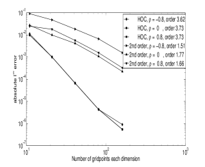
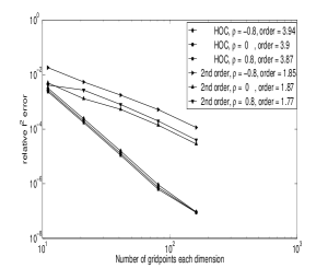
Figure 1: Absolute $l^{\infty}$-error and relative $l^{2}$-error for two-dimensional Black-Scholes Basket Put with smoothed initial condition.

In Fig. 1 we show plots of the $l^{\infty}$-error and the relative $l^{2}$-error. The high-order compact scheme performs highly similar for the three different correlation values, the points are almost identical. The numerical convergence orders for the high-order compact scheme range between $3.62$ and $3.73$ for the $l^{\infty}$-error, and between $3.87$ and $3.94$ for the relative $l^{2}$-error. The high-order compact scheme significantly outperforms the standard second-order discretisation in all cases.

References

- [1] Düring, B., Fournié, M.: High-order compact finite difference scheme for option pricing in stochastic volatility models. J. Comput. Appl. Math. 236(17), 4462–4473 (2012)
- [2] Düring, B., Fournié, M., Heuer, C.: High-order compact finite difference schemes for option pricing in stochastic volatility models on non-uniform grids. J. Comput. Appl. Math. 271(18), 247–266 (2014)
- [3] Düring, B., Heuer, C.: High-order compact schemes for parabolic problems with mixed derivatives in multiple space dimensions. Preprint (2014)
- [4] Karaa, S., Zhang, J.: Convergence and performance of iterative methods for solving variable coefficient convection-diffusion equation with a fourth-order compact difference scheme. Comput. Math. Appl. 44(3-4), 457–479 (2002)
- [5] Kreiss, H., Thomee, V., Widlund, O.: Smoothing of initial data and rates of convergence for parabolic difference equations. Commun. Pure Appl. Math. 23, 241–259 (1970)
- [6] Spotz, W., Carey, G.: Extension of high-order compact schemes to time-dependent problems. Numer. Methods Partial Differ. Equations 17(6), 657–672 (2001)
- [7] Tangman, D., Gopaul, A., Bhuruth, M.: Numerical pricing of options using high-order compact finite difference schemes. J. Comp. Appl. Math. 218(2), 270–280 (2008)
- [8] Wilmott, P.: Derivatives. The theory and practice of financial engineering. John Wiley & Sons Ltd., Chichester, UK (1998)