Rates of convergence for robust geometric inference

Abstract

Distances to compact sets are widely used in the field of Topological Data Analysis for inferring geometric and topological features from point clouds. In this context, the distance to a probability measure (DTM) has been introduced by Chazal et al., 2011b as a robust alternative to the distance a compact set. In practice, the DTM can be estimated by its empirical counterpart, that is the distance to the empirical measure (DTEM). In this paper we give a tight control of the deviation of the DTEM. Our analysis relies on a local analysis of empirical processes. In particular, we show that the rate of convergence of the DTEM directly depends on the regularity at zero of a particular quantile function which contains some local information about the geometry of the support. This quantile function is the relevant quantity to describe precisely how difficult is a geometric inference problem. Several numerical experiments illustrate the convergence of the DTEM and also confirm that our bounds are tight.

1 Introduction and motivation

The last decades have seen an explosion in the amount of available data in almost all domains of science, industry, economy and even everyday life. These data, often coming as point clouds embedded in Euclidean spaces, usually lie close to some lower dimensional geometric structures (e.g. manifold, stratified space,…) reflecting properties of the system from which they have been generated. Inferring the topological and geometric features of such multivariate data has recently attracted a lot of interest in both statistical and computational topology communities.

Considering point cloud data as independent observations of some common probability distribution $P$ in $\mathbb{R}^{d}$, many statistical methods have been proposed to infer the geometric features of the support of $P$ such as principal curves and surfaces Hastie and Stuetzle, (1989), multiscale geometric analysis Arias-Castro et al., (2006), density-based approaches Genovese et al., (2009) or support estimation, to name a few. Although they come with statistical guarantees these methods usually do not provide geometric guarantees on the estimated features.

On another hand, with the emergence of Topological Data Analysis (Carlsson,, 2009), purely geometric methods have been proposed to infer the geometry of compact subsets of $\mathbb{R}^{d}$. These methods aims at recovering precise geometric information of a given shape – see, e.g. Chazal and Lieutier, (2008); Niyogi et al., (2008); Chazal et al., 2009a ; Chazal et al., 2009b . Although these methods come with strong topological and geometric guarantees they usually rely on sampling assumptions that do not apply in statistical settings. In particular, these methods can be very sensitive to outliers. Indeed, they generally rely on the study of the sublevel sets of distance functions to compact sets. In practice only a sample drawn on, or close, to a geometric shape is known and thus only a distance to the data can be computed. The sup norm between the distance to the data and the distance to the underlying shape being exactly the Hausdorff distance between the data and the shape, we see that the statistical analysis of standards TDA methods boils down to the problem of support estimation in Hausdorff metric. This last problem has been the subject of much study in statistics (see for instance Devroye and Wise,, 1980; Cuevas and Rodríguez-Casal,, 2004; Singh et al.,, 2009). Being strongly dependent of the estimation of the support in Hausdorff metric, it is now clear why standard TDA methods may be very sensitive to outliers.

To provide a more robust approach of TDA, a notion of distance function to a measure (DTM) in $\mathbb{R}^{d}$ has been introduced by Chazal et al., 2011b as a robust alternative to the classical distance to compact sets. Given a probability distribution $P$ in $\mathbb{R}^{d}$ and a real parameter $0\leq u\leq 1$, Chazal et al., 2011b generalize the notion of distance to the support of $P$ by the function

$$\delta_{P,u}:x\in\mathbb{R}^{d}\mapsto\inf\{t>0\,;\,P(\bar{B}(x,t))\geq u\}$$ (1)

where $\bar{B}(x,t)$ is the closed Euclidean ball of center $x$ and radius $t$. For $u=0$, this function coincides with the usual distance function to the support of $P$. For higher values of $u$, it is larger than the usual distance function since a portion of mass $u$ has to be included in the ball centered on $x$. To avoid issues due to discontinuities of the map $P\to\delta_{P,u}$, the distance to measure (DTM) function with parameter $m\in[0,1]$ and power $r\geq 1$ is defined by

$$d_{P,m,r}(x):x\in\mathcal{\mathbb{R}}^{d}\mapsto\left(\frac{1}{m}\int_{0}^{m}\delta_{P,u}^{r}(x)du\right)^{1/r}.$$ (2)

It was shown in Chazal et al., 2011b that the DTM shares many properties with classical distance functions that make it well-adapted for geometric inference purposes (see Theorem 4 in Appendix A). First, it is stable with respect to perturbations of $P$ in the Wasserstein metric . This property implies that the DTM associated to close distributions in the Wasserstein metric have close sublevel sets. Moreover, when $r=2$, the function $d_{P,m,2}^{2}$ is semiconcave ensuring strong regularity properties on the geometry of its sublevel sets. Using these properties, Chazal et al., 2011b show that, under general assumptions, if $\tilde{P}$ is a probability distribution approximating $P$, then the sublevel sets of $d_{\tilde{P},m,2}$ provide a topologically correct approximation of the support of $P$. The introduction of DTM has motivated further works and applications in various directions such as topological data analysis Buchet et al., 2015a , GPS traces analysis Chazal et al., 2011a , density estimation Biau et al., (2011), deconvolution Caillerie et al., (2011) or clustering Chazal et al., (2013) just to name a few. Approximations, generalizations and variants of the DTM have also been recently considered in Guibas et al., (2013); Buchet et al., 2015b ; Phillips et al., (2014). However no strong statistical analysis of the DTM has not been proposed so far.

In practice, the measure $P$ is usually only known through a finite set of observations $\mathbb{X}_{n}=\{X_{1},\dots,X_{n}\}$ sampled from $P$, raising the question of the approximation of the DTM. A natural idea to estimate the DTM from $\mathbb{X}_{n}$ is to plug the empirical measure $P_{n}$ instead of $P$ in the definition of the DTM. This “plug-in strategy" corresponds to computing the distance to the empirical measure (DTEM). It can be applied with other estimators of the measure $P$, for instance in Caillerie et al., (2011) it was proposed to plug a deconvolved measure into the DTM.

For $m=\frac{k}{n}$, the DTEM satisfies

$$d^{r}_{P_{n},k/n,r}(x):=\frac{1}{k}\sum_{j=1}^{k}{\|x-\mathbb{X}_{n}\|}^{r}_{(j)}\,,$$

where $\|x-\mathbb{X}_{n}\|_{(j)}$ denotes the distance between $x$ and its $j$-th neighbor in $\{X_{1},\dots,X_{n}\}$. This quantity can be easily computed in practice since it only requires the distances between $x$ and the sample points.

Let us introduce

$$\Delta_{n,m,r}(x) := d^{r}_{P_{n},m,r}(x)-d^{r}_{P,m,r}(x)$$ (3)

and

$$\tilde{\Delta}_{n,m,r}(x):=d_{P_{n},r,m}(x)-d_{P,m,r}(x).$$

The aim of this paper is to study the deviations and the rate of convergence of $\Delta_{n,m,r}(x)$. The functional convergence of the DTEM has been studied recently in Chazal et al., 2014a where it is shown that the parametric convergence rate in $1/\sqrt{n}$ is achieved under reasonable assumptions. In this paper we address the question of the convergence in probability and the rate of convergence in expectation of $\Delta_{n,m,r}(x)$, both from an asymptotic and non asymptotic point perspective.

The stability properties of DTM with respect to Wasserstein metrics suggests that this problem could be addressed using known results about the convergence of empirical measure $P_{n}$ to $P$ under Wasserstein metrics. This last problem has been the subject of many works in the past (Rachev and Rüschendorf,, 1998; del Barrio et al.,, 1999, 2005) and it is still an active field of research (Fournier and Guillin,, 2013; Dereich et al.,, 2013). Contrary to the context of TDA with the standard distance function, where stability result provide optimal rates of convergence (see Chazal et al., (2015)), we show in the paper that Wasserstein stability does not lead to optimal results for the DTM. Moreover, such a basic approach does not provide a correct understanding of the influence of the parameter $m$ (see Appendix A).

We adopt an alternative approach based on the observation that the DTM only depends on a push forward measure of $P$ on the real line. Indeed, the DTM can be rewritten as follows:

$$d^{r}_{P,m,r}(x)=\frac{1}{m}\int_{0}^{m}F_{x,r}^{-1}(u)du,$$ (4)

where $F_{x,r}^{-1}$ is the quantile function of the push forward probability measure of $P$ by the function $\|x-\cdot\|^{r}$ (see appendix B.1 for a rigorous proof). Then we have

$$\Delta_{n,m,r}(x) := \frac{1}{m}\int_{0}^{m}\left\{F_{x,r,n}^{-1}(u)-F_{x,r}^{-1}(u)\right\}du,$$ (5)

where $F_{x,r,n}$ is the empirical distribution function of the observed distances (to the power $r$): ${\|x-X_{1}\|}^{r}$, $\dots$, ${\|x-X_{n}\|}^{r}$. We study the convergence of $\Delta_{n,m,r}(x)$ to zero with both an asymptotic and non asymptotic points of view. An asymptotic approach means that we take $k=k_{n}:=mn$ for some fixed $m$ and we study the mean rate of convergence to zero of $\Delta_{n,\frac{k_{n}}{n},r}(x)$. A non asymptotic approach means that $n$ is fixed and then the problem is to get a tight expectation bound on $\Delta_{n,\frac{k}{n},r}(x)$. In particular, we are particularly interested in the situation where $\frac{k}{n}$ is chosen very close to zero. This situation is of primary interest since it corresponds to the realistic situation where we use the DTM to clean the support from a small proportion of outliers.

Our results rely on a local analysis of the empirical process to compute tight deviation bounds of $\Delta_{n,\frac{k}{n},r}(x)$. More precisely, we use a sharp control of a supremum defined on the uniform empirical process. Such local analysis has been successfully applied in the literature about non asymptotic statistics, for instance Mammen et al., (1999) obtain fast rates of convergence in classification. For a more general presentation of these ideas in model selection, see Massart, (2007) and in particular Section 1.2 in the Introduction of this monograph.

We show that the rate of convergence of $\Delta_{n,\frac{k}{n},r}(x)$ directly depends on the regularity at zero of $F_{x,r}^{-1}$. This quantile function appears to be the relevant quantity to describe precisely how difficult is a geometric inference problem. The second contribution of this paper is relating the regularity of the quantile function $F_{x,r}^{-1}$ to the geometry of the support, establishing a link between the complexity of the geometric problem and a purely probabilistic quantity.

Our main results, the deviations bounds and the rate of convergence of $\Delta_{n,\frac{k}{n},r}(x)$ derived from the local analysis, are given in Section 2. These results are given in terms of the regularity of the quantile function $F_{x,r}^{-1}$. Generally speaking, it is not easy to determine what is the regularity of the quantile function $F_{x,r}^{-1}$ given a distribution $P$ and an observation point $x\in\mathbb{R}^{d}$. Indeed, it depends on the shape of the support of $P$, on the way the measure $P$ is distributed on its support and on the position of $x$ with regards to the support of $P$. This is why, in the results given in Section 2, the assumptions are made directly on the quantile functions $F_{x}^{-1}$. Section 3 is then devoted to the geometric interpretation of these results and their assumptions. In Section 4, several numerical experiments illustrate the convergence of the DTEM and also confirm that our bounds are sharp. Rates of convergence derived from stability results of the DTM are presented in Appendix A. Proofs and background about empirical processes and quantiles can be found in the appendices also.

Notation. Let $a\wedge b$ and $a\vee b$ denotes the minimum and the maximum between two real numbers $a$ and $b$. The Euclidean norm on $\mathbb{R}^{d}$ is $\|\cdot\|$. The open Euclidean ball of center $x$ and radius $t$ is denoted by $B(x,t)$. For some point $x$ and a compact set $K$ in $\mathbb{R}^{d}$, the distance between $x$ and $K$ is defined by $\|K-x\|:=\inf_{y\in K}\|y-x~\|$. The Hausdorff distance between two compact sets $K$ and $K^{\prime}$ is denoted by $\operatorname{Haus}\left(K,K^{\prime}\right)$. A probability distribution on $\mathbb{R}$ defined by a distribution function $F$ is denoted by $dF$. The quantile function $F^{-1}$ of $dF$ is defined by

$$F^{-1}(u):=\inf\{t\in\mathbb{R}\,,\,F(t)\geq u\},\quad 0<u<1.$$

By monotonicity, the quantile function $F^{-1}$ can be extended in $0$ and at $1$ by setting $F^{-1}(0)=\inf\{t\in\mathbb{R}\,,\,F(t)>0\},$ and $F^{-1}(1)=\sup\{t\in\mathbb{R}\,,\,F(t)<1\}.$ Finally, for two positive sequences $(a_{n})$ and $(b_{n})$, we use the standard notation $a_{n}\lesssim b_{n}$ if there exists a positive constant $C$ such that $a_{n}\leq Cb_{n}$.

2 Main results

We fix $r\geq 1$ and we henceforth write $F_{x}$ for $F_{x,r}$ to facilitate the reading. In the same way we will use the notation $F_{x}^{-1}$, $\tilde{\Delta}_{P,m}$, $d_{P,m}$ since there is no ambiguity on the power term $r$.

Given an observation point $x\in\mathbb{R}^{d}$, we introduce the modulus of continuity $\tilde{\omega}_{x}$ of $F_{x}^{-1}$ (possibly infinite) which is defined for any $v\in(0,1]$ by

$$\tilde{\omega}_{x}(v):=\sup_{(u,u^{\prime})\in[0,1]^{2},\,\|u-u^{\prime}\|\leq v}|F^{-1}_{x}(u)-F^{-1}_{x}(u^{\prime})|.$$

Note that the fact that $\tilde{\omega}_{x}$ is finite is equivalent to the fact that the support of $P$ is bounded. An extensive discussion about the relation between the measure $P$ and the modulus of continuity of $F_{x}^{-1}$ is proposed in Section 3. The function $\tilde{\omega}_{x}$ being non decreasing and non negative, it has a non negative limit $\tilde{\omega}_{x}(0^{+})$ at zero. In particular we do not assume here that $\tilde{\omega}_{x}(0^{+})=0$. In other terms we do not assume that $F_{x}^{-1}$ is continuous. We extend $\tilde{\omega}_{x}$ at zero by taking $\tilde{\omega}_{x}(0)=\tilde{\omega}_{x}(0^{+})$.

In the following, it will be sufficient in our results to consider upper bounds on the modulus of continuity, that is a non negative function $\omega_{x}$ on $[0,1]$ such that $\omega_{x}(v)\geq\tilde{\omega}(v)$ for any $v\in[0,1]$. A modulus of continuity being a non decreasing function, we will assume that such an upper bound $\omega_{x}$ is non decreasing on $[0,1]$. For technical reasons and without loss of generality, we will also assume that $\omega_{x}$ is a continuous function, which takes its values in $[\omega(0),\omega(1)]\subset\bar{\mathbb{R}}^{+}$. For such a function $\omega_{x}$ we also introduce its inverse function $\omega_{x}^{-1}$ which is defined on $[\omega(0),\omega(1)]$. We extend this function to $\mathbb{R}^{+}$ by taking $\omega_{x}^{-1}(t)=0$ for any $t\in[0,\omega(0)]$ and $\omega_{x}^{-1}(t)=1$ for any $t\geq\omega(1)$. In particular, $\omega_{x}^{-1}\left(\omega_{x}(u)\right)=u$ for any $u\in[0,1]$.

In this section, we show that the rate of convergence of $\Delta_{n,\frac{k}{n}}(x)$ is of the order of $\frac{\omega_{x}\left(\frac{k}{n}\right)}{\sqrt{k}}$.

2.1 Local analysis of the distance to the empirical measure in the bounded case

We first consider the behavior of the distance to the empirical measure when the observations $X_{1},\dots,X_{n}$ are sampled from a distribution $P$ with compact support in $\mathbb{R}^{d}$. Let $F_{x}^{-1}$ be the quantile function of $\|x-X_{1}\|^{r}$ and let $\Delta_{n,\frac{k}{n}}$ be defined by (3).

Theorem 1.

Let $x$ be a fixed observation point in $\mathbb{R}^{d}$. Assume that $\omega_{x}:[0,1]\rightarrow\mathbb{R}^{+}$ is an upper bound on the modulus of continuity of $F_{x}^{-1}$. Assume moreover that $\omega_{x}$ is an increasing and continuous function on $[0,1]$.

1. For any $\lambda>0$, if $k<\frac{n}{2}$ then

   $$\frac{P\left(|\Delta_{n,\frac{k}{n}}(x)|\geq\lambda\right)}{2}\leq\exp\left(-\frac{1}{64}\frac{k\lambda^{2}}{\left[F_{x}^{-1}\left(\frac{k}{n}\right)-F_{x}^{-1}(0)\right]^{2}}\right)+\exp\left(-\frac{3}{16}\frac{k\lambda}{F_{x}^{-1}\left(\frac{k}{n}\right)-F_{x}^{-1}(0)}\right)\\ +\exp\left(-\frac{n^{2}}{4k}\left\{\omega_{x}^{-1}\left(k^{1/4}\sqrt{\frac{\lambda}{8}\omega_{x}\left(\frac{2\sqrt{k}}{n}\right)}\right)\right\}^{2}\right)+\exp\left(-\frac{3n}{8}\omega_{x}^{-1}\left(k^{1/4}\sqrt{\frac{\lambda}{2}\omega_{x}\left(\frac{2\sqrt{k}}{n}\right)}\right)\right)\\ +\exp\left(-\frac{\sqrt{k}}{8}\frac{\lambda}{\omega_{x}\left(\frac{2\sqrt{k}}{n}\right)}\right)+\exp\left(-\frac{3k^{3/4}}{4}\sqrt{\frac{\lambda}{2\omega_{x}\left(\frac{2\sqrt{k}}{n}\right)}}\right):=\square(\lambda),$$ (6)

   otherwise

   $$\frac{P\left(|\Delta_{n,\frac{k}{n}}(x)|\geq\lambda\right)}{2}\leq\exp\left(-2n\lambda^{2}\left[\frac{\frac{k}{n}}{F^{-1}\left(\frac{k}{n}\right)-F^{-1}(0)}\right]^{2}\right)\\ +\exp\left(-2n\left\{\omega_{x}^{-1}\left(\sqrt{\frac{k}{\sqrt{n}}\omega_{x}\left(\frac{1}{\sqrt{n}}\right)\frac{\lambda}{2}}\right)\right\}^{2}\right)+\exp\left(-\frac{k}{\sqrt{n}\omega_{x}\left(\frac{1}{\sqrt{n}}\right)}\lambda\right).$$

   Furthermore, in all cases we have $P\left(|\Delta_{n,\frac{k}{n}}(x)|\geq\lambda\right)=0$ for any $\lambda>\omega_{x}(1)$.

2. Assume moreover that $\omega_{x}(u)/u$ is a non increasing function, then for any $k\in\{1,\dots,n\}$:

   $$\mathbb{E}\left(|\Delta_{n,\frac{k}{n}}(x)|\right) \leq \frac{C}{\sqrt{k}}\left\{\left[F_{x}^{-1}\left(\frac{k}{n}\right)-F_{x}^{-1}(0)\right]+\omega_{x}\left(\frac{\sqrt{k}}{n}\right)\right\}$$ (7)

   $$\leq \frac{2C}{\sqrt{k}}\omega_{x}\left(\frac{k}{n}\right),$$ (8)

   where $C$ is an absolute constant.

The proof of the Theorem is based on a particular decomposition of $\Delta_{n,\frac{k}{n}}(x)$, see Lemma 5 in Appendix B.1. This decomposition allows us to consider the deviations of the empirical process rather than the deviations of the quantile process. The proof is given in Appendix B.

Let us now comment on the final bound on expectation (8). This bound can be rewritten as follows:

$$\mathbb{E}\left|\Delta_{n,\frac{k}{n}}(x)\right|\lesssim\frac{n}{k}\frac{1}{\sqrt{n}}\sqrt{\frac{k}{n}}\omega_{x}\left(\frac{k}{n}\right).$$ (9)

The term $\frac{n}{k}$ comes from the definition of the DTM, it is the renormalization by the mass proportion $\frac{k}{n}$. The term $\frac{1}{\sqrt{n}}$ corresponds to a classical parametric rate of convergence. The term $\sqrt{\frac{k}{n}}$ is obtained thanks to a local analysis of the empirical process. More precisely, it derives from a sharp control of the variance of the supremum over the uniform empirical process. The term $\omega_{x}\left(\frac{k}{n}\right)$ corresponds to the statistical complexity of the problem, expressed in terms of the regularity of the quantile function $F_{x}^{-1}$.

Theorem 1 can be interpreted with either an asymptotic or a non asymptotic point of view. Taking a non asymptotic approach, we consider $n$ as fixed. A first result here is that we obtain sharp upper bounds for small values of $\frac{k}{n}$. In the most favorable case where $\tilde{\omega}_{x}(u)\sim u$, we see in (8) that an upper bound of the order of $\frac{1}{n}$ is reached. This is direct consequence of the local analysis we use to control the empirical process in the neighborhood of the origin. As mentioned before, assuming that $\frac{k}{n}$ is very small corresponds to the realistic situation where we use the DTM to clean the support from a small proportion of outliers.

Now, taking an asymptotic approach, a second result of Theorem 1 is that it allows us to consider the asymptotic behavior of $\Delta_{n,\frac{k}{n}}(x)$ under all possible regimes, that is for all sequences $(k_{n})_{n\in\mathbb{N}}$. For instance, with the classical approach where $k_{n}$ is such that $k_{n}/n=m$ for some fixed value $m\in(0,1)$, we then obtain the parametric rate of convergence $1/\sqrt{n}$, as in the asymptotic functional results given in Chazal et al., 2014a .

Another key fact about Theorem 1 is that the upper bound (7) depends on the regularity of $F_{x}^{-1}$ through the function

$$\Psi_{x}:m\in(0,1)~\mapsto\frac{\omega_{x}(m)}{\sqrt{m}}.$$

Moreover, if $\omega(0^{+})=0$, we see that the upper bound (7) depends on the regularity of $F_{x}^{-1}$ only at $0$ for $n$ large enough. For instance, if $k_{n}$ is such that $k_{n}/n=m$ for some fixed value $m\in(0,1)$ such that $F_{x}^{-1}(m)>F_{x}^{-1}(0)$, coming back to (7), we find that for $n$ large enough:

$$\omega_{x}\left(\frac{\sqrt{k_{n}}}{n}\right)=\omega_{x}\left(\frac{1}{\sqrt{n}}m\right)<F_{x}^{-1}\left(m\right)-F_{x}^{-1}(0).$$

In this context, the right hand term of Inequality (7) is of the order of $\frac{\widetilde{\Psi}_{x}(\frac{k_{n}}{n})}{\sqrt{k_{n}}}$ where

$$\widetilde{\Psi}_{x}:m\in(0,1)~\mapsto\frac{F_{x}^{-1}(m)-F_{x}^{-1}(0)}{\sqrt{m}}.$$

We now give additional remarks about Theorem 1.

Remark 1.

If the quantile function $F_{x}^{-1}$ is $\eta$-Hölder, then $\omega_{x}(u)=Au^{\eta}$ for some constant $A\geq 0$ and thus we have

$$\mathbb{E}\left(|\Delta_{n,\frac{k}{n}}(x)|\right)\lesssim\frac{1}{\sqrt{n}}\left[\frac{k}{n}\right]^{\eta-1/2}.$$

Remember that Hölder functions with power $\eta>1$ are constants, we can thus assume that $\eta\leq 1$.

Remark 2.

Assuming that $\omega_{x}(u)/u$ is a non increasing function roughly means that $\omega_{x}$ is a concave function. Our result is thus satisfied if we can find an concave function which is an upper bound on the modulus of continuity of the quantile function. We show in Section 3.4 that it is satisfied for a large class of measures.

Remark 3.

For values of $\frac{k}{n}$ not close to zero, the rate is consistent with the upper bound (15) deduced from the approach based on the stability results (see Appendix A). However, Theorem 1 is more satisfactory since it describes the statistical complexity of the problem through the regularity of the quantile function.

Remark 4.

The application $u\mapsto u^{1/r}$ is $1/r$- Hölder on $\mathbb{R}^{+}$ with Hölder constant $1$ since $1/r<1$. It yields:

$$|\tilde{\Delta}_{n,\frac{k}{n},r}(x)|\leq|\Delta_{n,\frac{k}{n},r}(x)|^{1/r}.$$ (10)

where $\tilde{\Delta}_{n,\frac{k}{n},r}(x)$ is defined by (1). We deduce an expectation bound on $\tilde{\Delta}_{n,\frac{k}{n},r}(x)$ from Jensen’s Inequality and Inequality (10):

$$\mathbb{E}\left(|\tilde{\Delta}_{n,\frac{k}{n},r}(x)|\right)\lesssim\left[\frac{1}{\sqrt{n}}\left[\frac{k}{n}\right]^{-1/2}\omega_{x}\left(\frac{k}{n}\right)\right]^{1/r}.$$

Remark 5.

As already mentioned before, to prove Theorem 1, we consider the deviations of the empirical process rather than the deviations of the quantile process. Indeed, the more direct approach that consists in directly controlling the deviations of the quantile process gives slower rates. More precisely, using Proposition 7 given in Appendix C borrowed from Shorack and Wellner, (2009), it can be shown that

$$\mathbb{E}\left(|\Delta_{n,\frac{k}{n}}(x)|\right)\lesssim\omega_{x}\left(\frac{\sqrt{k}}{n}\right).$$

For instance, if $\omega_{x}(u)=Au^{\eta}$, we obtain $\mathbb{E}\left(|\Delta_{n,\frac{k}{n},r}(x)|\right)\lesssim\left(\frac{\sqrt{k}}{n}\right)^{\eta}$ which is slower than the rate given in Remark 1.

To complete the results of Theorem 1, we give below a lower bound using Le Cam’s lemma (see Lemma 8 in Appendix C). Let $\omega$ be a continuous and increasing function on $[0,1]$ and let $x\in\mathbb{R}^{d}$. We introduce that class of probability measures:

$$\mathcal{P}_{\omega}:=\left\{P\>\textrm{is a probability measure on }\mathbb{R}^{d}\textrm{ such that }\omega(u)\geq\tilde{\omega}_{x}(u)\textrm{ for any }u\in[0,1]\right\}.$$

In the previous definition, the function $\tilde{\omega}$ is as before the modulus of continuity of the quantile function of the distribution of the push-forward measure of $P$ by the function $y\mapsto\|y-x\|^{r}$.

Proposition 1.

Assume that there exists $P\in\mathcal{P}_{\omega}$, $c>0$ and $\bar{u}\in(0,1)$, such that

$$c\left[F_{x}^{-1}(u)-F_{x}^{-1}(0)\right]\geq\omega(u)\quad\textrm{ for any }u\in(0,\bar{u}].$$ (11)

Then, there exits a constant $C$ which only depends on $c$, such that for any $k\leq\bar{u}n$.

$$\sup_{P\in\mathcal{P}_{\omega}}\mathbb{E}\left(|\Delta_{n,\frac{k}{n},r}(x)|\right) \geq \inf_{\hat{d}_{n}(x)}\sup_{P\in\mathcal{P}_{\omega}}\mathbb{E}\left(\left|\hat{d}_{n}^{r}(x)-d_{P,m,r}^{r}(x)\right|\right)$$

$$\geq C\frac{n}{k}\frac{1}{n}\omega\left(\frac{k-1}{n}\right),$$

where the infimum is than over all the estimator $\hat{d}_{n}(x)$ of $d_{P,m,r}(x)$ defined from a sample $X_{1},\dots,X_{n}$ of distribution $P$.

The Assumption (11) is not very strong. It means that $\omega$ is not a too large upper bound on the modulii of continuity of the quantile functions. More precisely, it says that there exists a distribution $P\in\mathcal{P}_{\omega}$ for which $\omega$ can be comparable to the modulus of continuity of the quantile functions $F_{x}^{-1}$ in the neighborhood of the origin.

Note that this lower bound matches with the upper bound of Theorem 1 when $k$ is very small since it is of the order of $\omega\left(\frac{k}{n}\right)$. Providing the correct lower bound for all values of $k$ is not obvious. As far as we know there is no standard method in the literature for computing lower bounds for this kind of functional and we consider that this issue is beyond the scope of this paper.

2.2 Local analysis of the distance to the empirical measure in the unbounded case

The previous results provide a description of the fluctuations and mean rates of convergence of the empirical distance to measure. However, when the support of $P$ is not bounded, the quantile function $F_{x}^{-1}$ tends to infinity at $1$ and the modulus of continuity of $F_{x}^{-1}$ is not finite. In such a situation, Theorem 1 can not be applied. We now propose a second result about the fluctuations of the DTEM, under weaker assumptions on the regularity of $F_{x}^{-1}$. The following result shows that under a weak moment assumption, the rate of convergence is the same as for the bounded case, up to a term decreasing exponentially fast to zero.

Theorem 2.

Let $\bar{m}\in(0,1)$ and some observation point $x\in\mathcal{\mathbb{R}}^{d}$. Assume that $\omega_{x,\bar{m}}$ is an upper bound of the modulus of continuity of $F_{x}^{-1}$ on $(0,\bar{m}]$: for any $u,u^{\prime}\in[0,\bar{m}]^{2}$,

$$|F^{-1}_{x}(u)-F^{-1}_{x}(u^{\prime})|\leq\omega_{x,\bar{m}}(|u-u^{\prime}|).$$ (12)

Assume moreover that $\omega_{x,\bar{m}}$ is increasing and continuous function on $[0,\bar{m}]$. Then, for any $k<n\left(\frac{1}{2}\wedge\bar{m}\right)$ and any $\lambda>0$:

$$\frac{P\left(|\Delta_{n,\frac{k}{n}}(x)|\geq\lambda\right)}{2}\leq\square(\lambda)+\exp\left(-\frac{\sqrt{k}}{8}\exp\left[\frac{n^{2}}{4k}\left(\bar{m}-\frac{k}{n}\right)^{2}\right]\lambda\right)\\ ~+\exp\left(-\frac{3}{8}\exp\left[\frac{n^{2}}{8k}\left(\bar{m}-\frac{k}{n}\right)^{2}\right]k^{\frac{3}{8}}\sqrt{\frac{\lambda}{2}}\right)\\ +\left\{2\exp\left(-\frac{n^{2}}{2k}\left\{\bar{m}-\frac{k}{n}\right\}^{2}\right)\right\}\wedge\left\{\frac{{n\choose k-1}}{2}\left[1-F\left(\sqrt{\frac{\lambda}{6}}\frac{k}{n}\right)\right]^{n-k+1}\right\}$$ (13)

where $\square(\lambda)$ is the upper bound given in Theorem 1, with $\omega_{x}$ replaced by $\omega_{x,\bar{m}}$. Assume moreover that $\omega_{x,\bar{m}}(u)/u$ is a non increasing function and that $P$ has a moment of order $r$. Then

$$\mathbb{E}\left|\Delta_{n,\frac{k}{n}}(x)\right|\leq\frac{C}{\sqrt{n}}\left[\frac{k}{n}\right]^{-1/2}\left\{\left[F_{x}^{-1}\left(\frac{k}{n}\right)-F_{x}^{-1}(0)\right]+\omega_{x,\bar{m}}\left(\frac{\sqrt{k}}{n}\right)\right\}+C_{x,r,\bar{m}}\sqrt{k}\exp\left[-\frac{n^{2}}{4k}\left(\bar{m}-\frac{k}{n}\right)^{2}\right].$$

where $C$ is an absolute constant and $C_{x,r,\bar{m}}$ only depends on the quantity $\mathbb{E}{\|X-x\|}^{r}$ and on $\bar{m}$.

As for the bounded case, if $\omega(0^{+})=0$ and if $F_{x}^{-1}(m)>F_{x}^{-1}(0)$, then the rate of convergence is still of the order of $\frac{\widetilde{\Psi}_{x}(m)}{\sqrt{n}}$. Note that this result is interesting even when the measure $P$ is supported on a compact set. Indeed, assume that the quantile function $F_{x}^{-1}$ is not continuous, then $\tilde{\omega}_{x}^{-1}(0)>0$. However, if $F_{x}^{-1}$ is smooth in the neighborhood of zero, for $\bar{m}$ small enough the assumption (12) may be satisfied with a function $\omega_{x,\bar{m}}$ which can be very small in the neighborhood of zero. Theorem 2 may provide better bounds in this context than those given by Theorem 1. This fact also confirms that the deviations of the DTEM mainly relies on the local regularity of the quantile function $F_{x}^{-1}$ at the origin rather then on its global regularity.

2.3 Convergence of the distance to the empirical measure for the sup norm

The previous results address the pointwise fluctuations of the DTEM. We now consider the same problem for the sup norm metric on a compact domain $\mathcal{D}$ of $\mathbb{R}^{d}$. Let $N(\mathcal{D},t)$ be the covering number of $\cal D$, that is the smallest number of balls $B(x_{i},t)$ with $x_{i}\in\cal D$, such that $\bigcup_{i}B(x_{i},t)\supset\cal D$. Since the domain $\cal D$ is compact, there exists two positive constants $c$ and $\nu\leq d$ such that for any $t>0$ :

$$N(\mathcal{D},t)\leq ct^{-\nu}\vee 1.$$

We assume that there exists a function $\omega_{\mathcal{D}}:(0,1]\rightarrow\mathbb{R}^{+}$ which uniformly upper bounds the modulus of continuity of the quantile functions $(F_{x}^{-1})_{x\in\mathcal{D}}$: for any $u,u^{\prime}\in(0,1]^{2}$ and for any $x\in\mathcal{D}$:

$$|F^{-1}_{x}(u)-F^{-1}_{x}(u^{\prime})|\leq\omega_{\cal D}(|u-u^{\prime}|).$$

We also assume as before that $\omega_{\mathcal{D}}$ is an increasing and continuous function on $[0,1]$.

Theorem 3.

Under the previous assumptions, for any $k\leq\frac{n}{2}$,

$$\mathbb{E}\left(\sup_{x\in\mathcal{D}}|\Delta_{n,\frac{k}{n}}(x)|\right) \leq \frac{C}{\sqrt{n}}\left[\frac{k}{n}\right]^{-1/2}\left[F_{x}^{-1}\left(\frac{k}{n}\right)-F_{x}^{-1}(0)\right]\log^{+}\left(\left[\frac{k}{\left[F_{x}^{-1}\left(\frac{k}{n}\right)-F_{x}^{-1}(0)\right]^{2}}\right]^{\nu+5}\right)$$

$$\hskip 28.45274pt+\>\frac{C}{\sqrt{n}}\left[\frac{k}{n}\right]^{-1/2}\omega_{\mathcal{D}}\left(\frac{\sqrt{k}}{n}\right)\log^{+}\left(\left[\frac{\sqrt{k}}{\omega_{\mathcal{D}}\left(\frac{\sqrt{k}}{n}\right)}\right]^{\nu-1}\right)$$

$$\leq \frac{C}{\sqrt{n}}\left[\frac{k}{n}\right]^{-1/2}\omega_{\mathcal{D}}\left(\frac{\sqrt{k}}{n}\right)\log^{+}\left(\frac{k^{\nu+5}}{\left[F_{x}^{-1}\left(\frac{\sqrt{k}}{n}\right)-F_{x}^{-1}(0)\right]^{2\nu+5}\wedge\left[\omega_{\mathcal{D}}\left(\frac{\sqrt{k}}{n}\right)\right]^{\nu-1}}\right)$$

where $\log^{+}(u)=(\log u)\vee 1$ for any $u\in\mathbb{R}^{+}$ . The constant $C$ is an absolute constant if $r=1$ otherwise it depends on $r$ and on the Hausdorff distance between $\cal D$ and the support of $P$.

This bound is deduced from a deviation bound on $\sup_{x\in\mathcal{D}}|\Delta_{n,\frac{k}{n}}(x)|$ which is given in the proof. Up to a logarithm term, the rate is the same as for the pointwise convergence. As for the pointwise convergence, this result could be easily extended to the case of non compactly supported measures.

3 The geometric information carried by the quantile function $\mathbf{F_{x}^{-1}}$

The upper bounds we obtain in the previous section directly depend on the regularity of $F_{x}^{-1}$. We now give some insights about how the geometry of the support of the measure in $\mathbb{R}^{d}$ impacts the quantile function $F_{x}^{-1}$.

3.1 Compact support and modulus of continuity of the quantile function

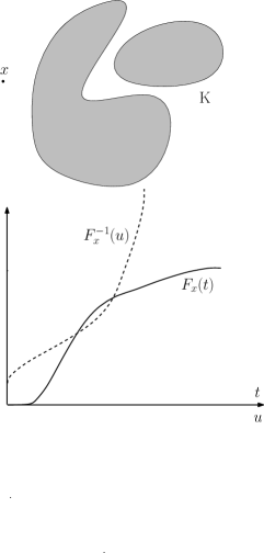
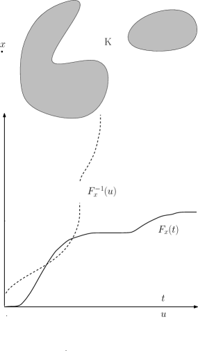
Figure 1: Left: one situation where the support of $P$ is not a connected set whereas the support of $dF_{x}$ is (for $r=1$). The quantile function $F_{x}^{-1}$ is continuous. Right: one situation where the support of $dF_{x}$ is is not a connected set ; the quantile function $F_{x}^{-1}$ is not continuous.

A geometric characterization of the existence of $\tilde{\omega}_{x}$ on $[0,1]$ can be given in terms of the support of the measure $P$. The following Lemma is borrowed and adapted from Proposition A.12 in Bobkov and Ledoux, (2014):

Lemma 1.

Given a measure $P$ in $\mathbb{R}^{d}$ and an observation point $x\in\mathbb{R}^{d}$, the following properties are equivalent:

1. the modulus of continuity of the quantile function $F^{-1}_{x}$ satisfies $\tilde{\omega}_{x}(u)<\infty$ for any $u\leq 1$ ;

2. the push-forward distribution of $P$ by the function $\|x-\cdot\|^{r}$ is compactly supported ;

3. $P$ is compactly supported.

In particular, if $P$ is compactly supported, we can always take as an upper bound on $\tilde{\omega}_{x}$ the constant function $\omega_{x}=\operatorname{Haus}\left(\{x\},K\right)$. Of course this is not a very relevant choice to describe the rate of convergence of the DTEM.

3.2 Connexity of the support and modulus of continuity of the quantile function

While discontinuity of the distribution function corresponds to atoms, discontinuity points of the quantile function corresponds to area with empty mass in $\mathbb{R}^{d}$ (see the right picture of Figure 1). The fact that $\tilde{\omega}_{x}(0^{+})=0$ is directly related to the connectedness of the support of the distribution $dF_{x}$. Indeed, it is equivalent to assuming that the support of $dF_{x}$ is a closed interval in $\mathbb{R}^{+}$, see for instance Proposition A.7 in Bobkov and Ledoux, (2014).

In the most favorable situations where the support of $P$ is a connected set, then $\tilde{\omega}_{x}(0^{+})=0$ and the faster $\tilde{\omega}_{x}$ tends to 0 at 0, the better the rate we obtain. However, for some point $x\in\mathbb{R}^{d}$, it is also possible for the support of $dF_{x}$ to be an interval even when the support of $P$ is not a connected set of $\mathbb{R}^{d}$ (see the left picture of Figure 1). In the other case, when the support of $dF_{x}$ is not a connected set, the term $\tilde{\omega}_{x}(0)$ roughly corresponds to the maximum distance between two consecutive intervals of the support of $dF_{x}$ (see the right picture of Figure 1). Our results can still be applied in these situations but the upper bounds we obtain in this case are larger because $\omega_{x}(\frac{k}{n})$ can not be smaller than $\tilde{\omega}_{x}(0)$.

3.3 Uniform modulus of continuity of $F_{x,r}^{-1}$ versus local continuity of $F_{x,r}^{-1}$ at the origin

Though stronger than continuity, a natural regularity assumption on $F_{x,r}^{-1}$ is assuming that this function is also concave:

Lemma 2.

If $F_{x}^{-1}$ is concave then we can take $\omega_{x}=F_{x}^{-1}-F_{x}^{-1}(0)$. In particular, if $x$ is in the support of $P$ then we can take $\omega_{x}=F_{x}^{-1}$.

If we take $r=1$, in many simple situations we note that the cumulative distribution function $F_{x,1}$ roughly behaves as a power function $t^{\ell}$, where $\ell$ is the dimension of the support. In this context, the quantile function $F_{x,1}^{-1}$ roughly behaves as a power function in $u^{1/\ell}$. We then have that $F_{x,r}^{-1}(u)=\left[F_{x,1}^{-1}(u)\right]^{r}$ behaves as $u^{\frac{r}{\ell}}$. This is for instance the case for $(a,b)$ standard measures, as shown in the next section. These considerations suggest that if $r/\ell<1$, in many situations the quantile function is concave and then $\omega_{x}$ is of the order of $F_{x}^{-1}-F_{x}^{-1}(0)$. This means that the upper bound on $\mathbb{E}|\Delta_{P,n,\frac{k}{n}}|~$ is of the order of $\frac{1}{\sqrt{n}}\widetilde{\Psi}_{x}(\frac{k}{n})$.

More generally, as noticed in the comments following Theorem 1, the term $F_{x}^{-1}(\frac{k}{n})-F_{x}^{-1}(0)$ is the dominating term in the upper bound (7). We may check with the numerical experiments of Section 4 that the function $\widetilde{\Psi}_{x}$ yet captures the correct monotonicity of $\mathbb{E}|\Delta_{P,n,\frac{k}{n}}|~$ as a function of $\frac{k}{n}$.

3.4 The case of $\mathbf{(a,b)}$ standard measures

The intrinsic dimensionality of a given measure in $\mathbb{R}^{d}$ can be quantified by the so-called $(a,b)$- standard assumption which assumes that there exists $a^{\prime}>0$, $\rho_{0}>0$ and $b>0$ such that

$$\forall x\in K,\ \forall r\in(0,\rho_{0}),\ P(B(x,\rho))\geq a^{\prime}\rho^{b},$$

where $K$ is the support of $P$. This assumption is popular in the literature about set estimation (see for instance Cuevas,, 2009; Cuevas and Rodríguez-Casal,, 2004). More recently, it has also been in used in Chazal et al., (2015); Fasy et al., (2014); Chazal et al., 2014b for statistical analysis inTopological Data Analysis.

Since $K$ is compact, by reducing the constant $a^{\prime}$ to a smaller constant $a$ if necessary, we easily check that this assumption (3.4) is equivalent to

$$\forall x\in K,\ P(B(x,\rho))\geq 1\wedge a\rho^{b}.$$

We now give control on the two key terms $\omega_{x}$ and $F_{x}^{-1}(u)-F_{x}^{-1}(0)$ which are involved in the bounds on expectations of Section 2.

Lemma 3.

Let $P$ be a probability measure on $\mathbb{R}^{d}$ which is $(a,b)$ standard on its support $K$. Then, for any $u\in[0,1]$,

$$F_{x}^{-1}(u)-F_{x}^{-1}(0)\leq r\left(\frac{u}{a}\right)^{1/b}\left[\left(\frac{u}{a}\right)^{1/b}+\|K-x\|\right]^{r-1},$$

where $r$ is the power parameter in the definition (2) of the DTM. Assume moreover that $K$ is a connected set of $\mathbb{R}^{d}$. Then, for any $h\in(0,1)$ we have

$$\tilde{\omega}_{x}(h)\leq r\left(\frac{h}{a}\right)^{1/b}\operatorname{Haus}\left(\{x\},K\right)^{r-1}.$$

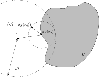
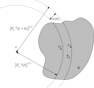
Figure 2: About the modulus of continuity of the quantile function $F_{x}^{-1}$ in the case of $(a,b)$- standard measures in $\mathbb{R}^{d}$.

Proof.

We have (see the left picture of Figure 2)

$$F_{x}(t) =P\left(B\left(x,t^{1/r}\right)\right)$$

$$\geq P\left(B\left(\pi_{K}(x),\left(t^{1/r}-\|K-x\|\right)^{+}\right)\right)$$

where $\pi_{K}(x)$ is a point of $\mathbb{R}^{d}$ which satisfies $\|K-x\|~=\|~\pi_{K}(x)-x\|$. Then $F_{x}(t)\geq a\left[\left(t^{1/r}-\|K-x\|\right)^{+}\right]^{b}$ and we find that $F_{x}^{-1}(u)\leq\left[\left(\frac{u}{a}\right)^{1/b}+\|K-x\|\right]^{r}$. Next, we have $F_{x}^{-1}(0)=\|K-x\|^{r}$ and the first point derives by upper bounding the derivatives of $v\mapsto\left[v+\|K-x\|\right]^{r}$.

We now assume that $K$ is a connected set. Let $(u,h)\in(0,1)^{2}$ such that $u+h\leq 1$ and $F_{x}^{-1}(u)>F_{x}^{-1}(0)$. We can also assume that $F_{x}^{-1}(u+h)>F_{x}^{-1}(u)$. Let $\alpha(h)=[F_{x}^{-1}(u+h)]^{1/r}-[F_{x}^{-1}(u)]^{1/r}$ (see the right picture of Figure 2). By definition of a quantile, there exists a point $x_{1}\in K\cap\left\{B\left(x,[F_{x}^{-1}(u+h)]^{1/r}\right)\setminus B\left(x,[F_{x}^{-1}(u)]^{1/r}\right)\right\}$. If $F_{x}^{-1}(u)>0$ then for the same reason there exists a point $x_{2}\in K\cap B\left(x,[F_{x}^{-1}(u)]^{1/r}\right)$. If $F_{x}^{-1}(u)=0$ then $x\in K$ and we take $x_{2}=x$. Next, since $K$ is a connected set, there exists a point $x_{3}\in K\cap B\left(x,[F_{x}^{-1}(t)]^{1/r}+\frac{\alpha}{2}\right)$. The measure $P$ being $(a,b)$-standard, we find that

$$h \geq P\left(B\left(x_{3},\frac{\alpha(h)}{2}\right)\right)$$

$$\geq a\left(\frac{\alpha(h)}{2}\right)^{b}.$$

Then,

$$[F_{x}^{-1}(t+h)]^{1/r}-[F_{x}^{-1}(t)]^{1/r}\leq\frac{2}{a^{1/b}}h^{1/b},$$

and thus

$$F_{x}^{-1}(t+h)-F_{x}^{-1}(t)\leq ra^{-1/b}\left(F_{x}^{-1}(t+h)\right)^{r-1}h^{1/b},$$

which proves the Lemma. ∎

4 Numerical experiments

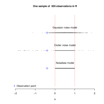
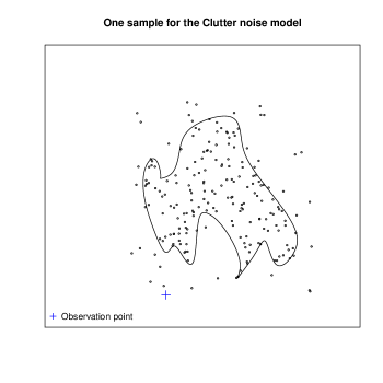
Figure 3: Left: samples drawn for each generative model for the Segment Experiment. Right: one sample drawn from the clutter noise model for the 2-d Shape Experiment. The observation point is represented by a blue cross.

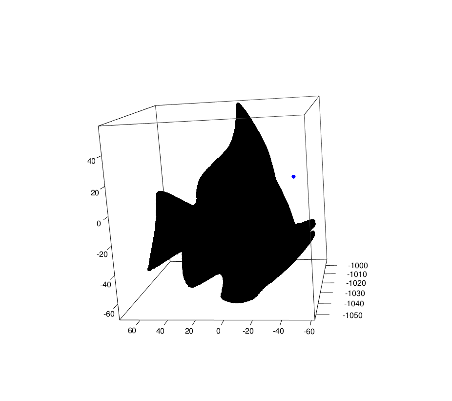
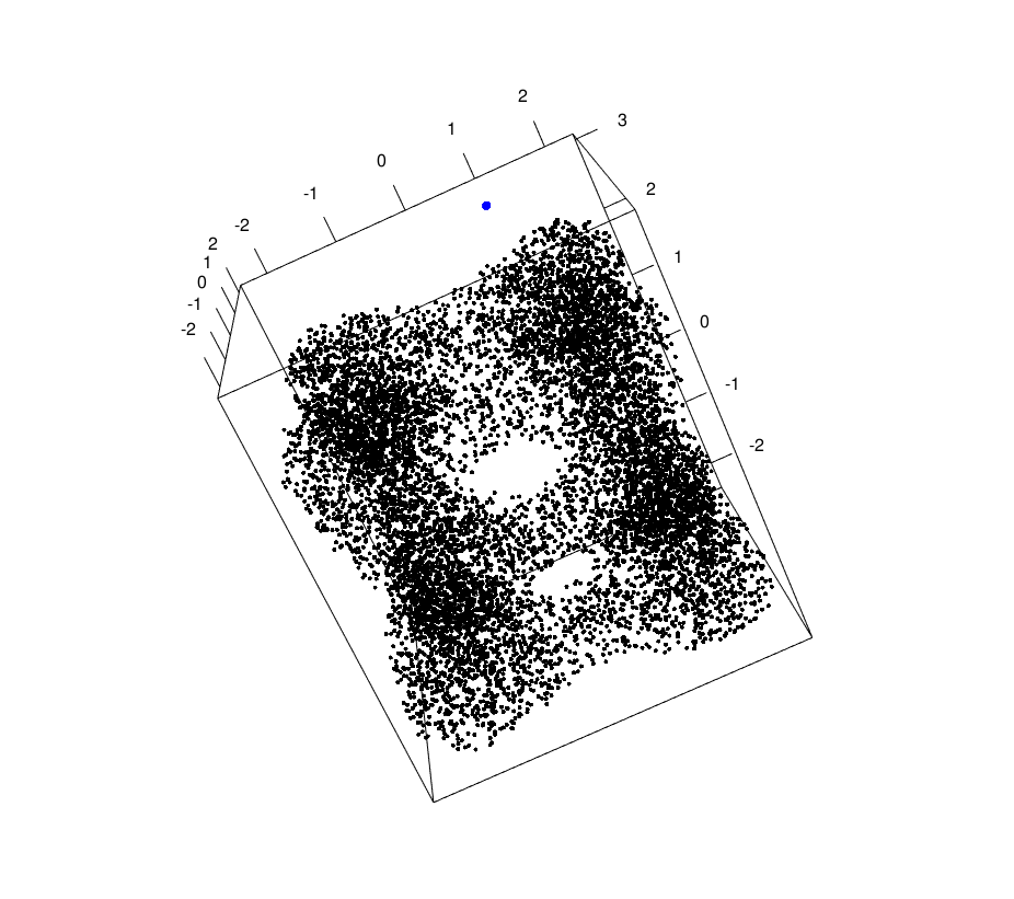
Figure 4: Left: 3-d plot of the shape for the Fish Experiment. Right: a 3-d plot of a sample drawn for the uniform measure on the Tangle Cube. The observation point is represented by the blue point outside of the shape.

In this section, we illustrate with numerical experiments that the expectation bounds given on $\Delta_{n,\frac{k}{n}}$ in Section 2 are sharp. In particular, we check that the function $\widetilde{\Psi}_{x}$ has the same monotonicity as the function $m\mapsto\mathbb{E}|\Delta_{n,\frac{k}{n}}(x)|~$.

We consider four different geometric shapes in $\mathbb{R}$, $\mathbb{R}^{2}$ and $\mathbb{R}^{3}$, for which a visualization is possible: see Figures 3 and 4.

• Segment Experiment in $\mathbb{R}$. The shape $K$ is the segment $[0,1]$ in $\mathbb{R}$.

• 2-d shape Experiment in $\mathbb{R}^{2}$. A closed curve has been drawn at hand in $\mathbb{R}^{2}$. It has been next approximated by a polygonal curve with a high precision. The shape $K$ is the compact set delimited by the polygon curve.

• Fish Experiment: a 2-d surface in $\mathbb{R}^{3}$. The shape $K$ is the discrete set defined by a point cloud of 216979 points approximating a 2-d surface representing a fish. This dataset is provided courtesy of CNR-IMATI by the AIM@SHAPE-VISIONAIR Shape Repository.

• Tangle Cube Experiment in $\mathbb{R}^{3}$. The shape $K$ is the tangle cube, that is the 3-d manifold defined as the set of points $(x_{1},x_{2},x_{3})\in\mathbb{R}^{3}$ such that $x_{1}^{4}-5x_{2}^{2}+x_{2}^{4}-5x_{2}^{2}+x_{3}^{4}-5x_{3}^{2}+10\leq 0$.

For each shape, we consider three generative models. These models are standard in support estimation and geometric inference, see Genovese et al., (2012) for instance.

• Noiseless model: $X_{1},\dots X_{n}$ are sampled from the uniform probability distribution $P_{uni}$ on $K$.

• Clutter noise model: $X_{1},\dots X_{n}$ are sampled from the mixture distribution $P_{cl}=\pi U+(1-\pi)P$ where $U$ is the uniform measure on a box $B$ which contains $K$ and where $\pi$ is a proportion parameter.

• Gaussian convolution model: $X_{1},\dots X_{n}$ are sampled from the distribution $P_{g}=P\star\Phi(0,\sigma I_{d})$ where $\Phi(0,\sigma)$ is the centered isotropic multivariate Gaussian distribution on $\mathbb{R}^{d}$ with covariance matrix $\sigma I_{d}$. We take $\sigma=0.5$ in all the experiments.

We use the same notation $P_{\mbox{\scriptsize$\square$}}$ for any of the probability distributions $P_{uni}$, $P_{cl}$ or $P_{g}$. An observation point $x$ is fixed for each experiment. For each experiment and each generative model, from a very large sample drawn from $P_{\square}$ we compute very accurate estimations of the quantile functions $F_{x,r}^{-1}$ and of the DTM $d_{P_{\square},m,t}(x)$. Next, we simulate $n$-samples from $P_{\square}$ and we compute the DTEM for each sample. We take $n=500$ for the two first experiments and $n=2000$ for the two others. The trials are all repeated 100 times and finally we compute some approximations of the error $\mathbb{E}\Delta_{n,\frac{k}{n},r}(x)$ with a standard Monte-Carlo procedure, for all the measures $P_{\square}$. The DTMs and the DTEMs are computed for the powers $r=1$, $r=2$ , and also for $r=3$ for the Tangle Cube Experiment. We also compute the function $m\mapsto\tilde{\Psi}(m)$. The simulations have been performed using R software (R Core Team,, 2014) and we have used the packages FNN, rgl, grImport and sp.

Results

The figures 5 to 8 give the results of the four experiments with the three generative models. The top graphics of Figures 5 to 8 represent the quantiles functions $F_{x,r}^{-1}$ in each case. For the noiseless models, the behavior of $F_{x,r}^{-1}$ at the origin is directly related to the power $r$ and to the intrinsic dimension of the shape. For $r=1$ , the quantile is linear for the the segment, it is roughly in $\sqrt{m}$ for the 2-d shape and for the Fish Experiment. It is of order of $m^{1/3}$ for the Tangle Cube. We observe that $F_{x,r}^{-1}$ is roughly linear with $r=2$ for the 2-d shape and the Fish shape, and with $r=3$ for the Tangle Cube.

The quantile functions of the noise models in the four cases start from zero since the observation is always taken inside the supports of $P_{cl}$ and $P_{g}$. A regularity break for the quantile function of the clutter noise model can be observed in the neighborhood of $m=P(B(x,\|K-x\|^{r}))$. The quantile functions for the Gaussian noise is always smoother.

The main point of these experiments is that, in all cases, the function $m\mapsto\tilde{\Psi}(m)$ shows the same monotonicity as the expected error studied in the paper $:m\mapsto|\mathbb{E}\Delta_{n,m,r}(x)|~$. These results confirm that the function $\tilde{\Psi}$ provides a correct description of $\mathbb{E}\Delta_{n,m,r}$.

We also observe that the function $:m\mapsto\mathbb{E}|\Delta_{n,m,r}(x)|~$ does not have one typical shape : it can be an increasing curve, a decreasing curve or even an U-shape curve. Indeed, the monotonicity depend on many factors including the intrinsic dimension of the shape, its geometry, the presence of noise and the power coefficient $r$.

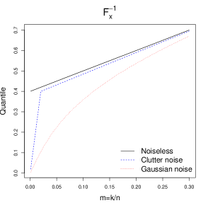
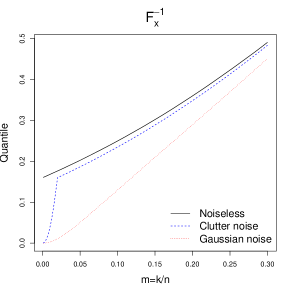
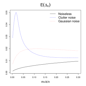
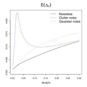
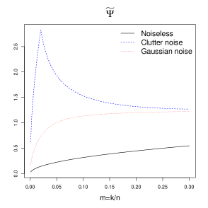
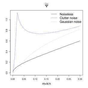
Figure 5: Quantiles functions $F_{x,r}^{-1}$ (top), expected error $\mathbb{E}\Delta_{n,\frac{k}{n},r}(x)$ (middle) and theoretical upper bounds $\tilde{\Psi}$ (bottom) with powers $r=1$ (left) and $r=2$ (right), for the Segment Experiment.

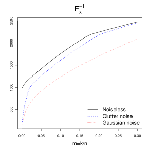
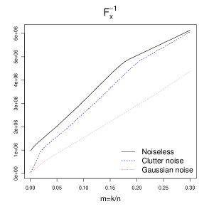
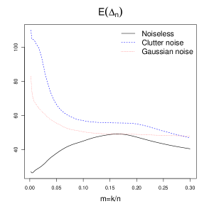
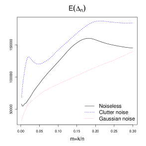
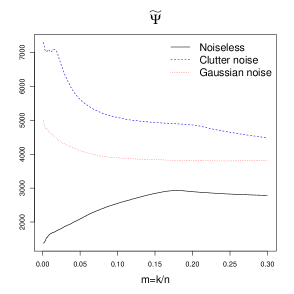
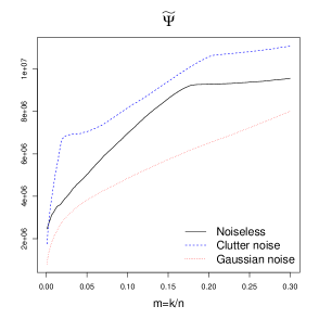
Figure 6: Quantiles functions $F_{x,r}^{-1}$ (top), expected error $\mathbb{E}\Delta_{n,\frac{k}{n},r}(x)$ (middle) and theoretical upper bounds $\tilde{\Psi}$ (bottom) with powers $r=1$ (left) and $r=2$ (right), for the 2-d Shape Experiment.

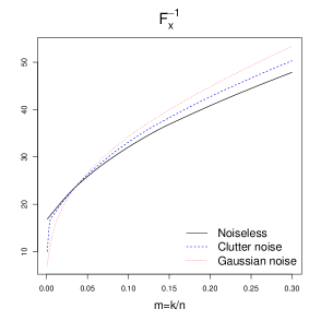
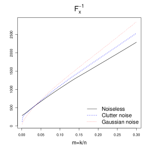
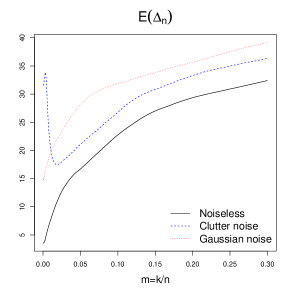
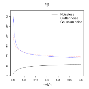
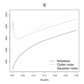
Figure 7: Quantiles functions $F_{x,r}^{-1}$ (top), expected error $\mathbb{E}\Delta_{n,\frac{k}{n},r}(x)$ (middle) and theoretical upper bounds $\tilde{\Psi}$ (bottom) with powers $r=1$ (left) and $r=2$ (right), for the Fish Experiment.

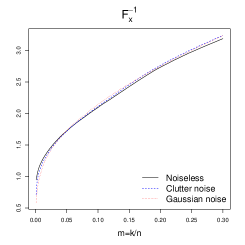
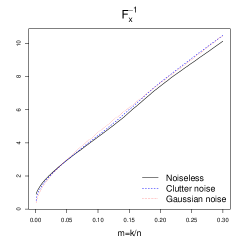
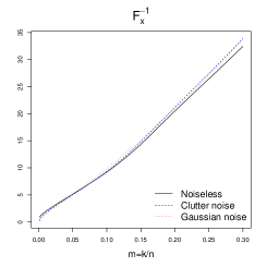
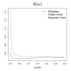
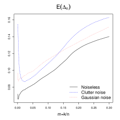
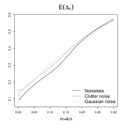
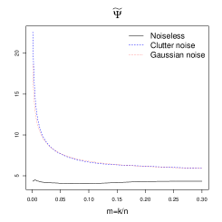
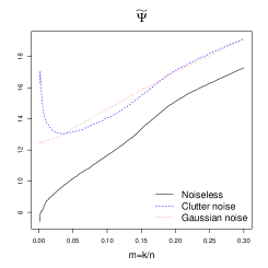
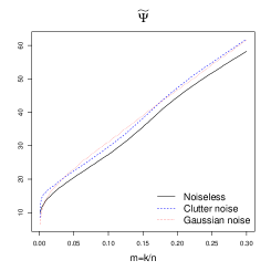
Figure 8: Quantiles functions $F_{x,r}^{-1}$ (top), expected error $\mathbb{E}\Delta_{n,\frac{k}{n},r}(x)$ (middle) and theoretical upper bounds $\tilde{\Psi}$ (bottom) with powers $r=1$ (left) and $r=2$ (right), for the Tangle Cube Experiment.

5 Conclusion

When the data is corrupted by noise, the distance to measure is one clue for performing robust geometric inference. For instance it can be used for support estimation and for topological data analysis using persistence diagrams, as proposed in Chazal et al., 2014a . In practice, a “plug-in" approach is adopted by replacing the measure by its empirical counterpart in the definition of the DTM. The main result of this paper is providing sharp non asymptotic bounds on the deviations of the DTEM.

The DTM has been recently extended to the context of metric spaces in Buchet et al., 2015b . For the sake of simplicity, we have assumed that $P$ is a probability measure in $\mathbb{R}^{d}$. However, all the results of the paper can be easily adapted to more general metric spaces by considering the push forward distribution of $P$ by $d(x,\cdot)^{r}$ where $d$ is the metric in the sampling space.

This paper is a step toward a complete theory about robust geometric inference. Our results give preliminary insights about how tuning the parameter $m$ in the DTEM, which is a difficult question. The experiments proposed in Section 4 show that the term $\mathbb{E}\Delta_{n,m,r}(x)$ does not have a typical monotonic behavior with regard to $m$ and thus classical model selection methods can be hardly applied to this problem. We intend to study this non standard model selection problem in future works.

Appendix A Rates of convergence derived from the DTM stability

The DTM satisfies several stability properties for the Wasserstein metrics. In this section, rates of convergence of the DTEM are derived from stability results of the DTM together with known results about the convergence of the empirical measure under Wasserstein metrics. We check that the results derived in this way are not as tight as the results given in Section 2.

Let us first remind the definition of the Wasserstein metrics in $\mathbb{R}^{d}$. For $r\geq 1$, the Wasserstein distance $W_{r}$ between two probability measures $P$ and $\tilde{P}$ on $\mathbb{R}^{d}$ is given by

$$W_{r}(P,\tilde{P})=\inf_{\pi\in\Pi(P,\tilde{P})}\left(\int_{\mathbb{R}^{d}\times\mathbb{R}^{d}}\|x-y\|^{r}\pi(dx,dy)\right)^{\frac{1}{r}},$$

where $\Pi(P,\tilde{P})$ is the set of probability measures on ${\mathbb{R}^{d}}\times{\mathbb{R}^{d}}$ with marginal distributions $P$ and $\tilde{P}$, see for instance Rachev and Rüschendorf, (1998) or Villani, (2008).

The stability of the DTM with respect to the Wasserstein distance $W_{r}$ is given by the following theorem.

Theorem 4 (Chazal et al., 2011b ).

Let $P$ and $\tilde{P}$ be two probability measures on $\mathbb{R}^{d}$. For any $r\geq 1$ and any $m\in(0,1)$ we have

$$\|d_{P,m,r}-d_{\tilde{P},m,r}\|_{\infty}\leq m^{-\frac{1}{r}}W_{r}(P,\tilde{P}).$$

Notice that  Chazal et al., 2011b prove this theorem for $r=2$, but the proof for any $r\geq 1$ is exactly the same.

We now give the pointwise stability of the DTM with respect to the Kantorovich distance $W_{1}$ between push forward measures on $\mathbb{R}$. This result easily derives from the expression (4) of the DTM given in Introduction, a rigorous proof is given in AppendixB.1.

Proposition 2.

For some point $x$ in $\mathbb{R}^{d}$ and some real number $r\geq 1$, let $dF_{x,r}$ and $d\tilde{F}_{x,r}$ be the push-forward measures by the function $y\mapsto\|x-y\|^{r}$ of two probability measures $P$ and $\tilde{P}$ defined on $\mathbb{R}^{d}$. Then, for any $x\in\mathbb{R}^{d}$:

$$\left|d_{P,m,r}^{r}(x)-d_{\tilde{P},m,r}^{r}(x)\right|\leq\frac{1}{m}W_{1}(dF_{x,r},d\tilde{F}_{x,r})\,.$$

Convergence results for $\Delta_{n,m,r}$ can be directly derived from the stability results given in Theorem 4 and Proposition 2. For instance, it can be easily checked that, for any $x\in\mathbb{R}^{d}$, $W_{1}(dF_{x,r},dF_{n,x})$ tends to zero almost surely (see for instance the Introduction Section of del Barrio et al.,, 1999). This together with Proposition 2 gives the almost surely pointwise convergence to zero of $\Delta_{n,m,r}(x)$.

Regarding the convergence in expectation, using Theorem 4 in $\mathbb{R}^{d}$ for $d>r/2$, we deduce from Fournier and Guillin, (2013) or from Dereich et al., (2013) that

$$\mathbb{E}\|\Delta_{n,\frac{k}{n},r}\|_{\infty} \leq \left(\frac{k}{n}\right)^{-1/r}\mathbb{E}W_{r}(P,P_{n})$$

$$\leq \left(\frac{k}{n}\right)^{-1/r}\left[\mathbb{E}W_{r}^{r}(P,P_{n})\right]^{1/r}$$

$$\leq C\left(\frac{k}{n}\right)^{-1/r}n^{-1/d}.$$

Nevertheless this upper bound is not sharp: assume that $k_{n}:=mn$ for some fixed constant $m\in(0,1)$ then the rate is of the order of $n^{-1/d}$. We show below that the parametric rate $1/\sqrt{n}$ can be obtained by considering the alternative stability result given in Proposition 2. In the one-dimensional case, a direct application of Fubini’s theorem gives that (see for instance Theorem 3.2 in Bobkov and Ledoux,, 2014)

$$\sqrt{n}\mathbb{E}\left[W_{1}(dF_{x,r},dF_{x,r,n})\right]\leq\int_{0}^{\infty}\sqrt{F_{x,r}(t)(1-F_{x,r}(t))}dt\>=:J_{1}(dF_{x,r}),$$ (14)

where $dF_{x,r}$ and $dF_{x,r,n}$ are the push forward probability measures of $P$ and $P_{n}$ by the function $\|x-\cdot\|^{r}$. Note that Bobkov and Ledoux, (2014) have completely characterized the convergence of $\mathbb{E}W_{1}(\mu,\mu_{n})$ in the one-dimensional case, in term of $J_{1}(\mu)$ for $\mu$ a probability measure on the real line and $\mu_{n}$ its empirical counterpart. From Proposition 2 and the upper bound (14) we derive that

$$\mathbb{E}\left|\Delta_{n,\frac{k}{n},r}(x)\right|\leq\frac{n}{k}\frac{J_{1}(dF_{x,r})}{\sqrt{n}}.$$ (15)

The integral $J_{1}(dF_{x,r})$ is finite if $\mathbb{E}\|X-x\|^{2r+\delta}<\infty$ for some $\delta>0$. We thus obtain a pointwise rate of convergence of $1/\sqrt{n}$ under reasonable moment conditions, if we take $k_{n}:=mn$ for some fixed constant $m\in(0,1)$. However, the upper bound (15) does not allow us to describe correctly how the rate depends on the parameter $m=\frac{k}{n}$. For instance, if $\frac{k}{n}$ is very small, the bound blows up in all cases while it should not be the case for instance with discrete measures. The reason is that the stability results are too global to provide a sharp expectation bound for small values of $\frac{k}{n}$.

Appendix B Proofs

B.1 Preliminary results for the DTM

Rewritting the DTM in terms of quantile function

Let $P$ a probability distribution in $\mathbb{R}^{d}$, $x\in\mathbb{R}^{d}$ and $r\geq 1$. Let $F_{x,r}$ be the distribution function of the random variable $\|x-X\|^{r}$, where the distribution of the random variable $X$ is $P$. The preliminary distance function to $P$

$$\delta_{P,u}:x\in\mathbb{R}^{d}\mapsto\inf\{t>0\,;\,P(\bar{B}(x,t))\geq u\}$$

can be rewritten in terms of the quantile function $F_{x,r}$:

Lemma 4.

For any $u\in(0,1)$, we have $\delta^{r}_{P,u}(x)=F_{x,r}^{-1}(u)$. In particular, $\delta_{P,u}(x)=F_{x,1}^{-1}(u)$.

Proof.

Note that for any $t\in\mathbb{R}^{+}$, $F_{x,r}(t)=P(B(x,{t}^{1/r}))$. Next,

$$\{t\geq 0\,;\,P(B(x,{t}^{1/r}))\geq\ell\}=\{s^{r}\,;s\geq 0\,,\,P(B(x,s))\geq\ell\}$$

and we deduce that

$$F_{x,r}^{-1}(\ell) = \inf\{s^{r}\,;s\geq 0\,,\,P(B(x,s))\geq\ell\}$$

$$= \delta^{r}_{P,\ell}(x).$$

where we have used the continuity of $s\mapsto s^{r}$ for the last equality. ∎

From Lemma 4 we directly derive the expression of the DTM in terms of the quantile function $F_{x,r}^{-1}$, as given by Equation (4) in the Introduction Section:

$$d^{r}_{P,m,r}(x)=\frac{1}{m}\int_{0}^{m}F_{x,r}^{-1}(u)du.$$

Proof of Proposition 4.

Let $F$ and $\tilde{F}$ be the cdfs of two probability measures $dF$ and $d\tilde{F}$ on $\mathbb{R}$. Recall that, for any $r\geq 1$, and any measure $\mu$ and $\tilde{\mu}$ in $\mathbb{R}$:

$$W_{r}^{r}(dF,d\tilde{F})=\int_{0}^{1}|\tilde{F}^{-1}(u)-F^{-1}(u)|^{r}du\,,$$ (16)

see for instance see for instance Vallender, (1974). Thus

$$\int_{0}^{m}|\tilde{F}^{-1}(u)-F^{-1}(u)|du\leq W_{1}^{r}(F,\tilde{F})$$

and the proof follows using Equation (4).

A decomposition of $\Delta_{n,\frac{k}{n},r}$.

For any $x\in\mathbb{R}^{d}$, any $r\geq 1$ we have $F_{x,n,r}^{-1}(0)\geq F_{x,r}^{-1}(0)\geq 0$ since $F_{x,r}$ is the cdf of the random distance $\|x-X\|^{r}$ whose support is included in $\mathbb{R}^{+}$. From Equation (5) and geometric considerations (see figure 9) we can rewrite $\Delta_{n,m,r}$ as given in the following Lemma.

Lemma 5.

The quantity $\Delta_{n,\frac{k}{n},r}$ can be rewritten as follows:

$$\Delta_{n,\frac{k}{n},r}(x) := \frac{n}{k}\int_{0}^{\frac{k}{n}}\left\{F_{x,n,r}^{-1}(u)-F_{x,r}^{-1}(u)\right\}du$$

$$= \frac{n}{k}\int_{F_{x,r}^{-1}(0)}^{F_{x,r}^{-1}(\frac{k}{n})\vee F_{x,n,r}^{-1}(\frac{k}{n})}\left\{F_{x,r}(t)\wedge\frac{k}{n}-F_{x,n,r}(t)\wedge\frac{k}{n}\right\}dt.$$

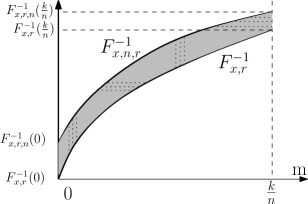
Figure 9: Calculation of $\Delta_{n,\frac{k}{n},r}(x)$ by integrating the grey domain horizontally or vertically.

B.2 Proof of Theorem 1

We recall that we use the notation $F$ for $F_{x,r}$ and $F_{n}$ for $F_{x,n,r}$ in the proof.

Upper bound on the fluctuations of $\Delta_{n,\frac{k}{n}}(x)$

We first check that $P\left(|\Delta_{n,\frac{k}{n}}(x)|\geq\lambda\right)=0$ for $\lambda\geq\omega_{x}(1)$. Note that $\omega_{x}(1)<\infty$ because the support of $P$ is compact. Let $\mathbb{G}_{n}$ and $\mathbb{G}^{-1}_{n}$ be the empirical uniform distribution function and the empirical uniform quantile function (see Appendix C). Starting from the definition (5) of the DTM and using Proposition 3 in Appendix C, we obtain that for $\lambda\geq 0$ and $k\leq n$:

$$P\left(|\Delta_{n,\frac{k}{n}}(x)|\geq\lambda\right) \leq P\left(\sup_{u\in[0,\frac{k}{n}]}\left|F^{-1}\left(\mathbb{G}^{-1}_{n}(u)\right)-F^{-1}(u)\right|\geq\lambda\right)$$

$$\leq P\left(\sup_{u\in[0,\frac{k}{n}]}\omega_{x}\left(\left|\mathbb{G}^{-1}_{n}(u)-u\right|\right)\geq\lambda\right)$$

$$\leq P\left(\sup_{u\in[0,\frac{k}{n}]}\left|\mathbb{G}^{-1}_{n}(u)-u\right|\geq\omega_{x}^{-1}(\lambda)\right),$$

and this probability is obviously zero for any $\lambda\geq\omega_{x}(1)$.

We now prove the deviation bounds starting from Lemma 5. If $F^{-1}(\frac{k}{n})\leq F_{n}^{-1}(\frac{k}{n})$, then

$$\Delta_{n,\frac{k}{n}}(x)=\frac{n}{k}\int_{F^{-1}(0)}^{F^{-1}(\frac{k}{n})}\left\{F(t)-F_{n}(t)\right\}dt+\frac{n}{k}\int_{F^{-1}(\frac{k}{n})}^{F_{n}^{-1}(\frac{k}{n})}\left\{\frac{k}{n}-F_{n}(t)\right\}dt$$

and thus

$$\left|\Delta_{n,\frac{k}{n}}(x)\right| \leq \underbrace{\frac{n}{k}\int_{F^{-1}(0)}^{F^{-1}(\frac{k}{n})}\left|F(t)-F_{n}(t)\right|dt}_{A}+\underbrace{\frac{n}{k}\int_{F^{-1}(\frac{k}{n})}^{F_{n}^{-1}(\frac{k}{n})}\left\{\frac{k}{n}-F_{n}(t)\right\}dt\>\mathbf{1}_{F_{n}^{-1}\left(\frac{k}{n}\right)\geq F^{-1}\left(\frac{k}{n}\right)}}_{B}$$ (17)

If $F^{-1}(\frac{k}{n})>F_{n}^{-1}(\frac{k}{n})$, then

$$\Delta_{n,\frac{k}{n}}(x)=\frac{n}{k}\int_{F^{-1}(0)}^{F_{n}^{-1}(\frac{k}{n})}\left\{F(t)-F_{n}(t)\right\}dt+\frac{n}{k}\int_{F_{n}^{-1}(\frac{k}{n})}^{F^{-1}(\frac{k}{n})}\left\{F(t)-\frac{k}{n}\right\}dt$$

and thus

$$\left|\Delta_{n,\frac{k}{n}}(x)\right| \leq \frac{n}{k}\int_{F^{-1}(0)}^{F_{n}^{-1}(\frac{k}{n})}\left|F(t)-F_{n}(t)\right|dt+\frac{n}{k}\int_{F_{n}^{-1}(\frac{k}{n})}^{F^{-1}(\frac{k}{n})}\left\{\frac{k}{n}-F(t)\right\}dt$$

$$\leq \frac{n}{k}\int_{F^{-1}(0)}^{F_{n}^{-1}(\frac{k}{n})}\left|F(t)-F_{n}(t)\right|dt+\frac{n}{k}\int_{F_{n}^{-1}(\frac{k}{n})}^{F^{-1}(\frac{k}{n})}\left\{F_{n}(t)-F(t)\right\}dt$$

$$\leq \frac{n}{k}\int_{F^{-1}(0)}^{F^{-1}(\frac{k}{n})}\left|F(t)-F_{n}(t)\right|dt.$$

In all cases, Inequality (17) is thus satisfied.

$\bullet$ Local analysis : deviation bound of $\Delta_{n,\frac{k}{n}}(x)$ for $\frac{k}{n}$ close to zero.

We now prove the deviation bound for $\frac{k}{n}<\frac{1}{2}$. We first upper bound the term A in (17). According to Proposition 5 in Appendix C, for any $u_{0}\in(0,\frac{1}{2})$ and any $\lambda>0$:

$$P\left(\sup_{u\in[0,u_{0}]}\left|\mathbb{G}_{n}(u)-u\right|\geq\lambda\right)\leq 2\exp\left(-\frac{n\lambda^{2}(1-u_{0})^{2}}{2u_{0}}\frac{1}{1+\frac{(1-u_{0})\lambda}{3u_{0}}}\right).$$ (18)

For $u_{0}\leq\frac{1}{2}$ and $\lambda>0$ it yields

$$P\left(\sup_{t\in\left[F^{-1}(0),F^{-1}(u_{0})\right)}\left|F_{n}(t)-F(t)\right|\geq\lambda\right) = P\left(\sup_{u\in[0,u_{0})}\left|\mathbb{G}_{n}(u)-u\right|\geq\lambda\right)$$

$$\leq 2\exp\left(-\frac{n\lambda^{2}(1-u_{0})^{2}}{2u_{0}}\frac{1}{1+\frac{(1-u_{0})\lambda}{3u_{0}}}\right)$$

$$\leq 2\exp\left(-\frac{n\lambda^{2}(1-u_{0})^{2}}{4u_{0}}\right)+2\exp\left(-\frac{3n\lambda(1-u_{0})}{4}\right),$$

where we have used Proposition 3 in Appendix C for the first equality, (18) for the second inequality, and that for any $u,v>0$, $\exp(-u/(1+v)\leq\exp(-u/2)+\exp(-u/(2v))$. The term $A$ can be upper bounded by controlling the supremum of $\left|F_{n}-F\right|$ over $\left[F^{-1}(0),F^{-1}\left(\frac{k}{n}\right)\right)$. If $\frac{k}{n}<\frac{1}{2}$, it yields

$$P\left(A\geq\lambda\right)\leq P\left(\frac{n}{k}\left[F^{-1}\left(\frac{k}{n}\right)-F^{-1}(0)\right]\sup_{t\in\left[F^{-1}(0),F^{-1}\left(\frac{k}{n}\right)\right)}\left|F_{n}(t)-F(t)\right|\geq\lambda\right)\\ \leq 2\exp\left(-\frac{n\lambda^{2}(1-\frac{k}{n})^{2}}{4\frac{k}{n}}\left[\frac{\frac{k}{n}}{F^{-1}\left(\frac{k}{n}\right)-F^{-1}(0)}\right]^{2}\right)+2\exp\left(-\frac{3n\lambda(1-\frac{k}{n})}{4}\left[\frac{\frac{k}{n}}{F^{-1}\left(\frac{k}{n}\right)-F^{-1}(0)}\right]\right)\\ \leq 2\exp\left(-\frac{n}{16}\frac{k}{n}\left[\frac{\lambda}{F^{-1}\left(\frac{k}{n}\right)-F^{-1}(0)}\right]^{2}\right)+2\exp\left(-\frac{3n}{8}\frac{k}{n}\frac{\lambda}{F^{-1}\left(\frac{k}{n}\right)-F^{-1}(0)}\right)$$ (19)

We now upper bound $B$. We have

$$B\leq\frac{n}{k}\left[F_{n}^{-1}\left(\frac{k}{n}\right)-F^{-1}\left(\frac{k}{n}\right)\right]\left[\frac{k}{n}-F_{n}\left(F^{-1}\left(\frac{k}{n}\right)\right)\right]\>\mathbf{1}_{F_{n}^{-1}\left(\frac{k}{n}\right)\geq F^{-1}\left(\frac{k}{n}\right)}.$$ (20)

Thus, according to Proposition 3 in Appendix C,

$$P(B\geq\lambda) \leq P\left(\frac{n}{k}\left\{\left[F^{-1}\left(\mathbb{G}_{n}^{-1}\left(\frac{k}{n}\right)\right)-F^{-1}\left(\frac{k}{n}\right)\right]\right\}\,\left\{\left[\frac{k}{n}-\mathbb{G}_{n}\left(\frac{k}{n}\right)\right]\right\}\>\mathbf{1}_{\mathbb{G}_{n}^{-1}\left(\frac{k}{n}\right)\geq\frac{k}{n}}\geq\lambda\right)$$

$$\leq P(B_{0}\geq\lambda)$$

where

$$B_{0}:=\left\{\sqrt{\frac{n}{k}}\omega_{x}\left(\,\mathbb{G}_{n}^{-1}\left(\frac{k}{n}\right)-\frac{k}{n}\right)\right\}\,\left\{\sqrt{\frac{n}{k}}\left[\frac{k}{n}-\mathbb{G}_{n}\left(\frac{k}{n}\right)\right]\right\}.$$

Let $\theta\in(0,1)$ to be chosen further. We have

$$2B_{0}\ \leq \underbrace{\left\{\theta\sqrt{\frac{n}{k}}\omega_{x}\left(\,\mathbb{G}_{n}^{-1}\left(\frac{k}{n}\right)-\frac{k}{n}\right)\right\}^{2}}_{B_{1}^{2}}\,+\,\underbrace{\left\{\frac{1}{\theta}\sqrt{\frac{n}{k}}\left[\frac{k}{n}-\mathbb{G}_{n}\left(\frac{k}{n}\right)\right]\right\}^{2}}_{B_{2}^{2}}$$

Then we can write

$$P(B\geq\lambda) \leq P\left(B_{1}\geq\sqrt{\lambda}\right)+P\left(B_{2}\geq\sqrt{\lambda}\right)$$

$$\leq P\left(\left|\mathbb{G}_{n}^{-1}\left(\frac{k}{n}\right)-\frac{k}{n}\right|\geq\omega_{x}^{-1}\left(\frac{\sqrt{\lambda}}{\theta}\sqrt{\frac{k}{n}}\right)\right)+P\left(\left|\mathbb{G}_{n}\left(\frac{k}{n}\right)-\frac{k}{n}\right|\geq\theta\sqrt{\lambda}\sqrt{\frac{k}{n}}\right).$$

Thus,

$$P(B\geq\lambda) \leq 2\exp\left(-\frac{n\left\{\omega_{x}^{-1}\left(\frac{\sqrt{\lambda}}{\theta}\sqrt{\frac{k}{n}}\right)\right\}^{2}}{4k/n}\right)+2\exp\left(-\frac{3n\omega_{x}^{-1}\left(\frac{\sqrt{\lambda}}{\theta}\sqrt{\frac{k}{n}}\right)}{8}\right)$$ (21)

$$+2\exp\left(-\frac{n^{2}\theta^{2}\left[\frac{k}{n}\right]\lambda}{4k}\right)+2\exp\left(-\frac{3\theta n}{4}\sqrt{\frac{k}{n}}\sqrt{\lambda}\right)$$

where we have used Propositions  4 and 6. According to (17), we have $P\left(\left|\Delta_{n,\frac{k}{n}}(x)\right|\geq\lambda\right)\leq P(A\geq\frac{\lambda}{2})+P(B\geq\frac{\lambda}{2})$. We then obtain the following deviation bound from Inequalities (19) and (21) for any $\frac{k}{n}<\frac{1}{2}$ and any $\lambda>0$:

$$\frac{P\left(|\Delta_{n,\frac{k}{n}}(x)|\geq\lambda\right)}{2}\leq\exp\left(-\frac{n}{64\left[F^{-1}\left(\frac{k}{n}\right)-F^{-1}(0)\right]^{2}}\frac{k}{n}\lambda^{2}\right)+\exp\left(-\frac{3n}{16}\frac{k}{n}\frac{\lambda}{F^{-1}\left(\frac{k}{n}\right)-F^{-1}(0)}\right)\\ +\exp\left(-\frac{n^{2}}{4k}\left\{\omega_{x}^{-1}\left(\frac{1}{\theta}{\sqrt{\frac{\lambda}{8}}}\sqrt{\frac{k}{n}}\right)\right\}^{2}\right)+\exp\left(-\frac{3n}{8}\omega_{x}^{-1}\left(\frac{1}{\theta}{\sqrt{\frac{\lambda}{2}}}\sqrt{\frac{k}{n}}\right)\right)\\ +\exp\left(-\frac{n\theta^{2}\lambda}{8}\right)+\exp\left(-\frac{3\theta n}{4}\sqrt{\frac{\lambda}{2}}\sqrt{\frac{k}{n}}\right),$$ (22)

where $\theta$ will be chosen further in the proof.

$\bullet$ Deviation bound of $\Delta_{n,\frac{k}{n}}(x)$ for $\frac{k}{n}\geq\frac{1}{2}$.

For controlling $A$, we now use the DKW Inequality (see Theorem 5), it gives that

$$P\left(A\geq\lambda\right) \leq P\left(\frac{n}{k}\left[F^{-1}\left(\frac{k}{n}\right)-F^{-1}(0)\right]\sup_{t\in[0,1]}\left|F_{n}(t)-F(t)\right|\geq\lambda\right)$$

$$\leq 2\exp\left(-2n\lambda^{2}\left[\frac{\frac{k}{n}}{F^{-1}\left(\frac{k}{n}\right)-F^{-1}(0)}\right]^{2}\right)$$

We decompose $B$ into $B_{1}$ and $B_{2}$ as before. We use DKW again for $B_{1}$ and $B_{2}$. For the quantile term $B_{1}$, note that

$$\left\{\sup_{u\in[0,\frac{k}{n}]}\left|\mathbb{G}_{n}^{-1}(u)-u\right|>\lambda\right\}\subset\left\{\sup_{u\in[0,1]}\left|\mathbb{G}_{n}^{-1}(u)-u\right|>\lambda\right\}=\left\{\sup_{t\in[0,1]}\left|\mathbb{G}_{n}(t)-t\right|>\lambda\right\}.$$

We find that for any $\tilde{\theta}>0$ :

$$\frac{P\left(|\Delta_{n,\frac{k}{n}}(x)|\geq\lambda\right)}{2}\leq\exp\left(-2n\lambda^{2}\left[\frac{\frac{k}{n}}{F^{-1}\left(\frac{k}{n}\right)-F^{-1}(0)}\right]^{2}\right)+\exp\left(-2n\left\{\omega_{x}^{-1}\left(\frac{1}{\tilde{\theta}}{\sqrt{\frac{\lambda}{2}}}\sqrt{\frac{k}{n}}\right)\right\}^{2}\right)\\ +\exp\left(-n\tilde{\theta}^{2}\lambda\frac{k}{n}\right).$$ (23)

where $\tilde{\theta}$ will be chosen further in the proof.

Upper bound on the expectation of $\Delta_{n,\frac{k}{n}}(x)$

$\bullet$ Case $\frac{k}{n}\leq\frac{1}{2}$.

By integrating the probability in (22), we obtain

$$\frac{\mathbb{E}\left||\Delta_{n,\frac{k}{n}}(x)\right|}{2}\leq 16\sqrt{\pi}\frac{1}{\sqrt{n}}\left(\frac{k}{n}\right)^{-\frac{1}{2}}\left[F^{-1}\left(\frac{k}{n}\right)-F^{-1}(0)\right]+\frac{16}{3n}\left(\frac{k}{n}\right)^{-1}\left[F^{-1}\left(\frac{k}{n}\right)-F^{-1}(0)\right]\\ +\underbrace{\int_{\lambda>0}\exp\left(-\frac{n^{2}}{4k}\left\{\omega_{x}^{-1}\left(\frac{1}{\theta}{\sqrt{\frac{\lambda}{2}}}\sqrt{\frac{k}{n}}\right)\right\}^{2}\right)\,d\lambda}_{I_{1}}+\underbrace{\int_{\lambda>0}\exp\left(-\frac{3n}{8}\omega_{x}^{-1}\left(\frac{1}{\theta}\sqrt{\frac{\lambda}{2}}\sqrt{\frac{k}{n}}\right)\right)\,d\lambda}_{I_{2}}\\ +\frac{8}{\theta^{2}n}+\frac{32}{9}\frac{1}{\theta^{2}n^{2}}\sqrt{\frac{n}{k}}$$ (24)

Since $\omega_{x}(u)/u$ is a non increasing function, we have that $\omega_{x}^{-1}(t)/t$ is a non decreasing function. Then, for any positive constants $\lambda_{1}$ and $\lambda_{2}$:

$$I_{1}+I_{2}\leq\lambda_{1}+\int_{\lambda>\lambda_{1}}\exp\left(-\frac{n^{2}}{4k}\left\{\frac{1}{\lambda_{1}}\omega_{x}^{-1}\left(\frac{1}{\theta}{\sqrt{\frac{\lambda_{1}}{2}}}\sqrt{\frac{k}{n}}\right)\right\}^{2}\lambda^{2}\right)\,d\lambda\\ +\lambda_{2}+\int_{\lambda>\lambda_{2}}\exp\left(-\frac{3n}{8\lambda_{2}}\omega_{x}^{-1}\left(\frac{1}{\theta}\sqrt{\frac{\lambda_{2}}{2}}\sqrt{\frac{k}{n}}\right)\lambda\right)\,d\lambda\\ =\left[\lambda_{1}+\frac{2\sqrt{k}}{n}\frac{\lambda_{1}}{\omega_{x}^{-1}\left(\frac{1}{\theta}{\sqrt{\frac{\lambda_{1}}{2}}}\sqrt{\frac{k}{n}}\right)}\right]+\left[\lambda_{2}+\frac{8\lambda_{2}}{3n\omega_{x}^{-1}\left(\frac{1}{\theta}\sqrt{\frac{\lambda_{2}}{2}}\sqrt{\frac{k}{n}}\right)}\right]$$

We then take $\lambda_{1}=2\left\{\theta\sqrt{\frac{n}{k}}\ \omega_{x}\left(\frac{2\sqrt{k}}{n}\right)\right\}^{2}$ and $\lambda_{2}=2\left\{\theta\sqrt{\frac{n}{k}}\omega_{x}\left(\frac{8}{3n}\right)\right\}^{2}$ and we find that

$$I_{1}+I_{2}\leq 4\left\{\theta\sqrt{\frac{n}{k}}\omega_{x}\left(\frac{2\sqrt{k}}{n}\right)\right\}^{2}+4\left\{\theta\sqrt{\frac{n}{k}}\omega_{x}\left(\frac{8}{3n}\right)\right\}^{2}.$$

We then choose

$$\theta^{2}=\frac{1}{\sqrt{n}\omega_{x}\left(\frac{2\sqrt{k}}{n}\right)}\sqrt{\frac{k}{n}}$$

to balance the terms $I_{1}$ and $\frac{8}{\theta^{2}n}$ in (24). The deviation bound given in the theorem corresponds to this choice for $\theta$.

Finally, note that $\omega_{x}\left(\frac{\sqrt{2k}}{n}\right)\leq\sqrt{2}\omega_{x}\left(\frac{\sqrt{k}}{n}\right)$ because $\omega_{x}(u)/u$ is a non increasing function and we obtain that there exists an absolute constant $C$ such that

$$\mathbb{E}\left|\Delta_{n,\frac{k}{n}}(x)\right|\leq\frac{C}{\sqrt{n}}\left[\frac{k}{n}\right]^{-1/2}\left\{\left[F^{-1}\left(\frac{k}{n}\right)-F^{-1}(0)\right]+\omega_{x}\left(\frac{\sqrt{k}}{n}\right)\right\}.$$ (25)

$\bullet$ Case $\frac{k}{n}\geq\frac{1}{2}$.

We integrate the deviations (23) and we obtain that

$$\mathbb{E}\left|\Delta_{n,\frac{k}{n}}(x)\right|\leq C\left[\frac{1}{\sqrt{n}}\left[\frac{F^{-1}\left(\frac{k}{n}\right)-F^{-1}(0)}{\frac{k}{n}}\right]+\left\{\tilde{\theta}\sqrt{\frac{n}{k}}\omega_{x}\left(\frac{1}{\sqrt{n}}\right)\right\}^{2}+\frac{1}{\tilde{\theta}^{2}n}\frac{n}{k}\right].$$ (26)

We then choose

$$\tilde{\theta}^{2}=\frac{1}{\sqrt{n}\omega_{x}\left(\frac{1}{\sqrt{n}}\right)}.$$

The deviation bound given in the Theorem correspond to this choice for $\tilde{\theta}$. Since $\sqrt{\frac{n}{k}}\leq\sqrt{2}\leq 2$, we see that the expectation bound (26) for this choice of $\tilde{\theta}$ can be rewritten as the expectation bound (25). This concludes the proof of Theorem 1.

B.3 Proof of Proposition 1

Figure 10: The two quantile functions $F_{0}^{-1}$ and $F_{1}^{-1}$.

We first consider the case $d=1$. For applying Le Cam’s Lemma (Lemma 8), we need to find two probabilities $P_{0}$ and $P_{1}$ which distances to measure are sufficiently far from each other. Without loss of generality we can assume that $x=0$. Let $\bar{P}\in\mathcal{P}_{\omega}$ which satisfies (11). We can assume that $\bar{P}$ is supported on $\mathbb{R}^{+}$ since the push forward measure of $\bar{P}$ by the norm is in $\mathcal{P}_{\omega}$ and also satisfies (11). Let $\bar{F}^{-1}$ be the quantile function of $\bar{P}$. For some $n\geq 1$, let $P_{0}:=\bar{P}$ and let $P_{1}:=\frac{1}{n}\delta_{0}+\left.\bar{P}\right|_{[0,\bar{F}^{-1}(1-1/n)]}$, where $\delta_{0}$ is a Dirac distribution at zero and where $\left.\bar{P}\right|_{[a,b]}$ is the restriction of the measure $\bar{P}$ to the set $[a,b]$. For $i=0,1$, let $P_{i,r}$ be the push-forward measure of $P_{i}$ by the power function $t\mapsto t^{r}$ on $\mathbb{R}^{+}$. Let also $F_{i,r}$ and $F_{i,r}^{-1}$ be the distribution function and the quantile function of $P_{i,r}$, see Figure 10 for an illustration. Note that that $P_{1,r}=\frac{1}{n}\delta_{0}+\left.P_{0,r}\right|_{[0,F_{0,r}^{-1}(1-1/n)]}$. Thus $P_{1}$ is in $\mathcal{P}_{\omega}$ because

$$F_{1,r}^{-1}(u)=\left\{\begin{array}[]{ll}F_{0,r}^{-1}(0)&\textrm{ if }u\leq\frac{1}{n},\\ F_{0,r}^{-1}(u-1/n)&\textrm{ otherwise.}\end{array}\right.$$

The probability measures $P_{0}$ and $P_{1}$ are absolutely continuous with respect to the measure $\mu:=\delta_{0}+\bar{P}$. The density of $P_{0}$ with respect to $\mu$ is $p_{0}:=\mathbf{1}_{(0,+\infty)}$ whereas the density of $P_{1}$ with respect to $\mu$ is $p_{1}=\frac{1}{n}\mathbf{1}_{\{0\}}+\mathbf{1}_{(0,\bar{F}^{-1}(1-1/n)]}$. Thus,

$$TV(P_{0},P_{1}) = \int_{\mathbb{R}^{+}}|p_{1}(t)-p_{0}(t)|\;d\mu(t)$$

$$= \frac{1}{n}+\bar{P}\left(\left(\bar{F}^{-1}\left(1-\frac{1}{n}\right),\infty\right)\right)$$

$$= \frac{2}{n}.$$

The next, $\left[1-TV(P_{0},P_{1})\right]^{2n}=(1-\frac{2}{n})^{2n}\rightarrow e^{-4}$ as $n$ tends to infinity. Moreover,

$$\left|d_{P_{0},r}^{r}(x)-d_{P_{1},r}^{r}(x)\right| = \frac{n}{k}\int_{0}^{\frac{k}{n}}\left\{F_{0,r}^{-1}(u)-F_{1,r}^{-1}(u)\right\}du$$

$$\geq \frac{n}{k}\int_{F_{1,r}^{-1}(u-1/n)}^{F_{1,r}^{-1}(\frac{k}{n})}\left\{F_{1,r}(t)-F_{0,r}(t)\right\}dt$$

according to basic geometric calculations. Thus,

$$\left|d_{P_{0},r}^{r}(x)-d_{P_{1},r}^{r}(x)\right| \geq \frac{n}{k}\frac{1}{n}\left[F_{1,r}^{-1}\left(\frac{k}{n}\right)-F_{1,r}^{-1}(0)\right]$$

$$\geq \frac{n}{k}\frac{1}{n}\left[F_{0,r}^{-1}\left(\frac{k}{n}\right)-F_{0,r}^{-1}(0)\right]$$

$$\geq \frac{n}{k}\frac{c}{n}\omega\left(\frac{k}{n}\right).$$

where we have used Assumption(11) for the last inequality. We conclude using Le Cam’s Lemma.

We now consider the case $d\geq 2$. Let $\bar{P}\in\mathcal{P}_{\omega}$ which satisfies (11). By considering the push-forward measure of $\bar{P}$ by the function

$$\begin{array}[]{rcl}\mathbb{R}^{d}&\longrightarrow&\mathbb{R}^{+}\times\{0\}^{d-1}\\ y&\longmapsto&(\|y\|,0,\dots,0)\\ \end{array}\,,$$

we see that it is aways possible to assume that there exist a probability $\bar{P}$ supported on $\mathbb{R}^{+}\times\{0\}^{d-1}$ which satisfies (11). Now, it is then possible to define $P_{0}$ and $P_{1}$ as in the case $d=1$ except that their support is now in $\mathbb{R}^{+}\times\{0\}^{d-1}$. Following the same construction, the quantities $TV(P_{0},P_{1})$ and $d_{P_{0},r}^{r}(x)-d_{P_{1},r}^{r}(x)$ take the same values as in the case $d=1$. We thus obtain the same lower bound as in the case $d=1$.

B.4 Proof of Theorem 2

Inequality (17) in the proof of Theorem 2 is still valid. We can also use the deviation bound (19) on $A$ for the case $\frac{k}{n}\leq\frac{1}{2}$. Regarding the deviation bound on $B$, we restart from Inequality (20) and we note that

$$\frac{n}{k}\left\{\left[F^{-1}\left(\mathbb{G}_{n}^{-1}\left(\frac{k}{n}\right)\right)-F^{-1}\left(\frac{k}{n}\right)\right]\right\}\,\left\{\left[\frac{k}{n}-\mathbb{G}_{n}\left(\frac{k}{n}\right)\right]\right\}\>\mathbf{1}_{\mathbb{G}_{n}^{-1}\left(\frac{k}{n}\right)\geq\frac{k}{n}}\\ \leq\frac{n}{k}\left\{\left[F^{-1}\left(\mathbb{G}_{n}^{-1}\left(\frac{k}{n}\right)\right)-F^{-1}\left(\frac{k}{n}\right)\right]\right\}\,\left\{\left[\frac{k}{n}-\mathbb{G}_{n}\left(\frac{k}{n}\right)\right]\right\}\>\mathbf{1}_{\frac{k}{n}\leq\mathbb{G}_{n}^{-1}\left(\frac{k}{n}\right)\leq\bar{m}}\\ +\frac{n}{k}\left\{\left[F^{-1}\left(\mathbb{G}_{n}^{-1}\left(\frac{k}{n}\right)\right)-F^{-1}\left(\frac{k}{n}\right)\right]\right\}\,\left\{\left[\frac{k}{n}-\mathbb{G}_{n}\left(\frac{k}{n}\right)\right]\right\}\>\mathbf{1}_{\mathbb{G}_{n}^{-1}\left(\frac{k}{n}\right)>\bar{m}}\\ \leq\underbrace{\frac{n}{k}\left\{\omega_{x}^{-1}\left(\mathbb{G}_{n}^{-1}\left(\frac{k}{n}\right)-\frac{k}{n}\right)\right\}\,\left\{\left[\frac{k}{n}-\mathbb{G}_{n}\left(\frac{k}{n}\right)\right]\right\}\>\mathbf{1}_{\mathbb{G}_{n}^{-1}\left(\frac{k}{n}\right)\leq\bar{m}}}_{\tilde{B}}\\ +\underbrace{\frac{n}{k}\left\{F^{-1}\left(\mathbb{G}_{n}^{-1}\left(\frac{k}{n}\right)\right)\right\}\,\left\{\left[\frac{k}{n}-\mathbb{G}_{n}\left(\frac{k}{n}\right)\right]\right\}\>\mathbf{1}_{\mathbb{G}_{n}^{-1}\left(\frac{k}{n}\right)>\bar{m}}}_{B_{3}}$$

By definition of $B$, $\tilde{B}$ and $B_{3}$, and using Proposition 3 in Appendix C, we obtain that

$$P\left(|\Delta_{n,\frac{k}{n}}(x)|\geq\lambda\right) \leq P\left(A\geq\frac{\lambda}{2}\right)+P\left(B\geq\frac{\lambda}{2}\right)$$ (27)

$$\leq P\left(A\geq\frac{\lambda}{2}\right)+P\left(\tilde{B}\geq\frac{\lambda}{2}\right)+P\left(B_{3}\geq\frac{\lambda}{2}\right)$$

where $P\left(A\geq\frac{\lambda}{2}\right)+P\left(\tilde{B}\geq\frac{\lambda}{2}\right)$ has already been upper bounded in the Proof of Theorem 2. We now upper bound the deviations of $B_{3}$. For any $\theta_{3}\in(0,1)$ to be chosen further, we have:

$$2B_{3}\leq\underbrace{\left\{\theta_{3}F^{-1}\left(\mathbb{G}_{n}^{-1}\left(\frac{k}{n}\right)\right)\right\}^{2}\>\mathbf{1}_{\mathbb{G}_{n}^{-1}\left(\frac{k}{n}\right)>\bar{m}}}_{B_{4}^{2}}\,+\,\underbrace{\left\{\frac{1}{\theta_{3}}\frac{n}{k}\left[\frac{k}{n}-\mathbb{G}_{n}\left(\frac{k}{n}\right)\right]\right\}^{2}}_{B_{5}^{2}}.$$

We have $P(B_{3}\geq\frac{\lambda}{2})\leq P\left(B_{4}\geq\sqrt{\frac{\lambda}{2}}\right)+P\left(B_{5}\geq\sqrt{\frac{\lambda}{2}}\right)$ where

$$P\left(B_{5}\geq\sqrt{\frac{\lambda}{2}}\right)\leq 2\exp\left(-\frac{k\theta_{3}^{2}\lambda}{8}\right)+2\exp\left(-\frac{3\theta_{3}k}{8}\sqrt{\frac{\lambda}{2}}\right).$$ (28)

The probability $P\left(B_{4}\geq\sqrt{\frac{\lambda}{4}}\right)$ can be upper bounded in two different ways: one using a concentration argument et one based on the Beta distribution of $\mathbb{G}_{n}^{-1}$. According to Proposition 6, we have

$$P\left(B_{4}\geq\sqrt{\frac{\lambda}{2}}\right) \leq P\left(\mathbb{G}_{n}^{-1}\left(\frac{k}{n}\right)-\frac{k}{n}\geq F\left(\sqrt{\frac{\lambda}{2}}\frac{1}{\theta_{3}}\right)\vee\bar{m}-\frac{k}{n}\right)$$ (29)

$$\leq 4\exp\left[-\frac{n^{2}}{2k}\left(\bar{m}-\frac{k}{n}\right)^{2}\right].$$

Next, it is well known (see for instance p.97 in Chapter 3 of Shorack and Wellner,, 2009) that $\mathbb{G}_{n}^{-1}\left(\frac{k}{n}\right)$ has a Beta$(k,n-k+1)$ distribution with density on $[0,1]$:

$$t\mapsto\frac{n!}{(k-1)!(n-k)!}t^{k-1}(1-t)^{n-k}.$$

Thus, for any $t\in(0,1)$, $P\left(\mathbb{G}_{n}^{-1}\left(\frac{k}{n}\right)\geq 1-t\right)\leq{n\choose k-1}t^{n-k+1}$. Thus

$$P\left(B_{4}\geq\sqrt{\frac{\lambda}{2}}\right) \leq P\left(B_{4}>\sqrt{\frac{\lambda}{3}}\right)$$ (30)

$$\leq P\left(\mathbb{G}_{n}^{-1}\left(\frac{k}{n}\right)>F\left(\sqrt{\frac{\lambda}{3}}\frac{1}{\theta_{3}}\right)\vee\bar{m}\right)$$

$$\leq {n\choose k-1}\left[1-F\left(\sqrt{\frac{\lambda}{3}}\frac{1}{\theta_{3}}\right)\vee\bar{m}\right]^{n-k+1}$$

where the first inequality allows us to deal with a strict comparaison, which is necessary to rewrite the probability in terms of the cdf. Note that a similar bound can be obtained using Bennett’s inequality for $B_{4}$.

We now upper bound $\mathbb{E}|\Delta_{n,\frac{k}{n}}(x)|$. We only need to control the deviations of $B_{3}$. Since $P$ has a moment of order $r$, for any $t>0$:

$$t\left(1-F(t)\right)=tP\left({\|x-X\|}^{r}>t\right)\leq\mathbb{E}{\|x-X\|}^{r}=:C_{x,r}.$$

Then for any $\bar{\lambda}>0$ (and $n$ larger than $3$):

$$\int_{0}^{\infty}P\left(B_{4}\geq\sqrt{\frac{\lambda}{2}}\right)d\lambda \leq 4\int_{0}^{\bar{\lambda}}\exp\left[-\frac{n^{2}}{2k}\left(\bar{m}-\frac{k}{n}\right)^{2}\right]d\lambda+{n\choose k-1}\int_{\bar{\lambda}}^{\infty}\left[1-F\left(\sqrt{\frac{\lambda}{3}}\frac{1}{\theta_{3}}\right)\right]^{n-k+1}d\lambda$$

$$\leq 4\bar{\lambda}\exp\left[-\frac{n^{2}}{2k}\left(\bar{m}-\frac{k}{n}\right)^{2}\right]+2^{n}\left[\sqrt{3}C_{x,r}\theta_{3}\right]^{n-k+1}\int_{\bar{\lambda}}^{\infty}\lambda^{\frac{-n+k-1}{2}}d\lambda$$

$$\leq 4\bar{\lambda}\exp\left[-\frac{n^{2}}{2k}\left(\bar{m}-\frac{k}{n}\right)^{2}\right]+\frac{8\bar{\lambda}}{n}\left[\frac{4\sqrt{3}C_{x,r}\theta_{3}}{\sqrt{\bar{\lambda}}}\right]^{n-k+1}$$

$$\leq 4\bar{\lambda}\left\{\exp\left[-\frac{n^{2}}{2k}\left(\bar{m}-\frac{k}{n}\right)^{2}\right]+\exp\left[-(n-k+1)\log\left(\frac{4\sqrt{3}C_{x,r}\theta_{3}}{\sqrt{\bar{\lambda}}}\right)\right]\right\}$$

We choose $\bar{\lambda}$ to balance the two terms inside the brackets:

$$\bar{\lambda}=\left\{4\sqrt{3}C_{x,r}\theta_{3}\log\left[\frac{n^{2}}{2k(n-k+1)}\left(\bar{m}-\frac{k}{n}\right)^{2}\right]\right\}^{2}$$

and then

$$\int_{0}^{\infty}P\left(B_{3}\geq\frac{\lambda}{2}\right)d\lambda \leq \int_{0}^{\infty}P\left(B_{4}\geq\sqrt{\frac{\lambda}{2}}\right)d\lambda+\int_{0}^{\infty}P\left(B_{5}\geq\sqrt{\frac{\lambda}{2}}\right)d\lambda$$

$$\leq C_{x,r,\bar{m}}\left\{\frac{1}{k\theta_{3}^{2}}+\theta_{3}^{2}\exp\left[-\frac{n^{2}}{2k}\left(\bar{m}-\frac{k}{n}\right)^{2}\right]\right\}$$

where $C_{x,r,\bar{m}}$ only depends on $C_{x,r}$ and $\bar{m}$. We thus take $\theta_{3}^{2}=\frac{\exp\left[\frac{n^{2}}{4k}\left(\bar{m}-\frac{k}{n}\right)^{2}\right]}{\sqrt{k}}$ and we obtain that

$$\int_{0}^{\infty}P\left(B_{3}\geq\frac{\lambda}{2}\right)d\lambda\leq C_{x,r,\bar{m}}\sqrt{k}\exp\left[-\frac{n^{2}}{4k}\left(\bar{m}-\frac{k}{n}\right)^{2}\right].$$

The deviation bound given in the Theorem derives from (27), (28), (29) and (30) with this value for $\theta_{3}$.

B.5 Proof of Theorem 3

We first recall the following Lemma from Chazal et al., 2011b .

Lemma 6 (Chazal et al., 2011b ).

For any $(x,y)\in(\mathbb{R}^{d})^{2}$ and any $m\in(0,1)$:

$$|d_{P,m,r}(x)-d_{P,m,r}(y)|\leq\|x-y\|.$$

Next Lemma directly derives from Lemma 6.

Lemma 7.

For $r=1$, the function $x\mapsto\Delta_{n,m,1}(x)$ is $1$- Lipschitz on $\mathbb{R}^{d}$. For $r>1$, the function $x\mapsto\Delta_{n,m,r}(x)$ is $C_{\mathcal{D},r}$ -Lipschitz on the compact domain $\mathcal{D}$ where $C_{\mathcal{D},r}$ depends on $r$ and on the Hausdorff distance between $\cal D$ and the support of $P$.

We give the proof of the Theorem for $r=1$. The calculations are also valid $r>1$ by replacing $\lambda$ by $\lambda C_{\mathcal{D},r}$ in the probability bounds. The deviation bound of the Theorem can be proved with a simple union bound strategy. Up to enlarging the constant $c$, we can write

$$N(\mathcal{D},\lambda)\leq c\lambda^{-\nu}\quad\textrm{for any }\lambda\leq\omega_{\cal D}(1).$$

Now, for a given $\lambda\leq\omega_{\cal D}(1)$, there exists an integer $N\leq c\lambda^{-\nu}$ and $N$ points $(x_{1},\dots,x_{N})$ laying in $\mathcal{D}$ such that $\bigcup_{i=1\dots N}B(x_{i},\lambda)\supseteq\mathcal{D}$. For any point $x\in\mathcal{D}$, there exists a point $\pi_{\lambda}(x)$ of $\{x_{1},\dots,x_{N}\}$ such that $\|x-\pi_{\lambda}(x)\|\leq\frac{\lambda}{2}$. According to Lemma 7, we have

$$|\Delta_{n,\frac{k}{n},1}(x)-\Delta_{n,\frac{k}{n},1}(\pi_{\lambda}(x))|\leq\frac{\lambda}{2}.$$ (31)

According to Theorem 1, we have for any $k<\frac{n}{2}$ and any $\lambda>0$:

$$P\left(\sup_{i=1\dots N}|\Delta_{n,\frac{k}{n},1}(x_{i})|\geq\frac{\lambda}{2}\right)\leq\left\{\begin{array}[]{lll}1\wedge 2c\lambda^{-\nu}\square(\lambda)&\textrm{if }\lambda\leq\omega_{\cal D}(1),\\ 0&\textrm{if }\lambda>2\omega_{\cal D}(1),\end{array}\right.$$ (32)

where

$$\square(\lambda)=\exp\left(-\frac{1}{64}\frac{k\lambda^{2}}{\left[F_{x}^{-1}\left(\frac{k}{n}\right)-F_{x}^{-1}(0)\right]^{2}}\right)+\exp\left(-\frac{3}{16}\frac{k\lambda}{F_{x}^{-1}\left(\frac{k}{n}\right)-F_{x}^{-1}(0)}\right)\\ +\exp\left(-\frac{n^{2}}{4k}\left\{\omega_{\mathcal{D}}^{-1}\left(k^{1/4}\sqrt{\frac{\lambda}{8}\omega_{\mathcal{D}}\left(2\frac{\sqrt{k}}{n}\right)}\right)\right\}^{2}\right)+\exp\left(-\frac{3n}{8}\omega_{\mathcal{D}}^{-1}\left(k^{1/4}\sqrt{\frac{\lambda}{2}\omega_{\mathcal{D}}\left(\frac{2\sqrt{k}}{n}\right)}\right)\right)\\ +\exp\left(-\frac{\sqrt{k}}{8}\frac{\lambda}{\omega_{\mathcal{D}}\left(\frac{2\sqrt{k}}{n}\right)}\right)+\exp\left(-\frac{3k^{3/4}}{4}\sqrt{\frac{\lambda}{2\omega_{\mathcal{D}}\left(\frac{2\sqrt{k}}{n}\right)}}\right)\\ =:\square_{1}(\lambda)+\square_{2}(\lambda)+\square_{3}(\lambda)+\square_{4}(\lambda)+\square_{5}(\lambda)+\square_{6}(\lambda).$$

Using (31) and (32), we find that $P\left(\sup_{x\in\mathcal{D}}|\Delta_{n,\frac{k}{n}}(x)|\geq\lambda\right)$ is also upper bounded by the right hand term of (32).

We now integrate each term in $\lambda^{-\nu}\square(\lambda)$. For the first one, let $\alpha_{k,n}=\frac{1}{64}\frac{k}{\left[F_{x}^{-1}\left(\frac{k}{n}\right)-F_{x}^{-1}(0)\right]^{2}}$, then for any $\lambda_{k,n}>0$:

$$\int_{0}^{\infty}1\wedge 2c\lambda^{-\nu}\square_{1}(\lambda)d\lambda \leq \lambda_{k,n}+2c\lambda_{k,n}^{-\nu}\int_{\lambda_{k,n}}^{\infty}\exp\left(-\alpha_{k,n}\lambda^{2}\right)d\lambda$$

$$\leq \lambda_{k,n}+2c\frac{\lambda_{k,n}^{-\nu-1}}{\alpha_{k,n}}\exp(-\alpha_{k,n}\lambda_{k,n}^{2}).$$

We balance these two terms by taking $\lambda_{n}=\sqrt{\frac{\log^{+}\left(\left[\alpha_{k,n}\right]^{\nu+5}\right)}{2\alpha_{k,n}}}$, it gives:

$$\int_{0}^{\infty}1\wedge 2c\lambda^{-\nu}\square_{1}(\lambda)d\lambda\lesssim\sqrt{\frac{\log^{+}\left(\left[\alpha_{k,n}\right]^{+5}\right)}{\alpha_{k,n}}}.$$ (33)

The upper bound for the second term can be obtained in the same way. For the third term, let $\beta_{k,n}:=k^{1/4}\sqrt{\frac{1}{8}\omega_{\mathcal{D}}\left(\frac{2\sqrt{k}}{n}\right)}$. Since $\omega_{\mathcal{D}}^{-1}(t)/t$ is non decreasing, for any $\lambda_{k,n}>0$:

$$\int_{0}^{\infty}1\wedge 2c\lambda^{-\nu}\square_{3}(\lambda)d\lambda \leq \lambda_{k,n}+2c\lambda_{k,n}^{-\nu}\int_{\lambda_{k,n}}^{\infty}\exp\left(-\frac{n^{2}\left\{\omega_{\mathcal{D}}^{-1}\left(\beta_{k,n}\sqrt{\lambda}\right)\right\}^{2}}{4k}\right)d\lambda$$

$$\leq \lambda_{k,n}+2c\lambda_{k,n}^{-\nu}\int_{\lambda_{k,n}}^{\infty}\exp\left(-\frac{n^{2}}{4k}\left\{\frac{\omega_{\mathcal{D}}^{-1}\left(\beta_{k,n}\sqrt{\lambda_{k,n}}\right)}{\sqrt{\lambda_{k,n}}}\right\}^{2}\lambda\right)d\lambda$$

$$\leq \lambda_{k,n}+4c\frac{k}{n^{2}}\frac{\lambda_{k,n}^{-\nu}}{\left\{\omega_{\mathcal{D}}^{-1}\left(\beta_{k,n}\sqrt{\lambda_{k,n}}\right)\right\}^{2}}\exp\left(-\frac{n^{2}}{4k}\left\{\omega_{\mathcal{D}}^{-1}\left(\beta_{k,n}\sqrt{\lambda_{k,n}}\right)\right\}^{2}\right).$$

We balance the two terms in the upper bounds by taking

$$\lambda_{k,n}=\left\{\frac{1}{\beta_{k,n}}\omega_{\mathcal{D}}\left(\frac{2\sqrt{k}}{n}\sqrt{\log^{+}\left(\left[\frac{\beta_{k,n}}{\omega_{\mathcal{D}}\left(\frac{2\sqrt{k}}{n}\right)}\right]^{2(\nu-1)}\right)}\right)\right\}^{2}.$$

Indeed, we then obtain that:

$$\int_{0}^{\infty}1\wedge 2c\lambda^{-\nu}\square_{3}(\lambda)d\lambda\lesssim\lambda_{k,n}+\\ \frac{\lambda_{k,n}}{\log^{+}\left(\left[\frac{\beta_{k,n}}{\omega_{\mathcal{D}}\left(\frac{2\sqrt{k}}{n}\right)}\right]^{2(\nu-1)}\right)}\left\{\frac{1}{\beta_{k,n}}\omega_{\mathcal{D}}\left(\frac{2\sqrt{k}}{n}\sqrt{\log^{+}\left(\left[\frac{\beta_{k,n}}{\omega_{\mathcal{D}}\left(\frac{2\sqrt{k}}{n}\right)}\right]^{2(\nu-1)}\right)}\right)\right\}^{-2(\nu-1)}\left[\frac{\omega_{\mathcal{D}}\left(\frac{2\sqrt{k}}{n}\right)}{\beta_{k,n}}\right]^{2(\nu-1)}\\ \lesssim\lambda_{k,n}+\lambda_{k,n}\left\{\omega_{\mathcal{D}}\left(\frac{2\sqrt{k}}{n}\sqrt{\log^{+}\left(\left[\frac{\beta_{k,n}}{\omega_{\mathcal{D}}\left(\frac{2\sqrt{k}}{n}\right)}\right]^{2(\nu-1)}\right)}\right)\right\}^{-2(\nu-1)}\times\\ \left[\omega_{\mathcal{D}}\left(\frac{2\sqrt{k}}{n}\sqrt{\log^{+}\left(\left[\frac{\beta_{k,n}}{\omega_{\mathcal{D}}\left(\frac{2\sqrt{k}}{n}\right)}\right]^{2(\nu-1)}\right)}\right)\right]^{2(\nu-1)}\\ \lesssim\lambda_{k,n}$$

where we have used $\log^{+}\geq 1$ and the fact that $\omega_{\mathcal{D}}(u)$ is non decreasing for the second inequality. Since $\omega_{\mathcal{D}}(u)/u$ is non increasing and $\log^{+}\geq 1$, we find that

$$\lambda_{k,n}\lesssim k^{-1/2}\left[\omega_{\mathcal{D}}\left(\frac{\sqrt{k}}{n}\right)\right]^{-1}\left\{\omega_{\mathcal{D}}\left(\frac{\sqrt{k}}{n}\right)\sqrt{\log^{+}\left(\left[\frac{\sqrt{k}}{\omega_{\mathcal{D}}\left(\frac{\sqrt{k}}{n}\right)}\right]^{\nu-1}\right)}\right\}^{2}\\ \lesssim\frac{\omega_{\mathcal{D}}\left(\frac{\sqrt{k}}{n}\right)}{\sqrt{k}}\log^{+}\left(\left[\frac{\sqrt{k}}{\omega_{\mathcal{D}}\left(\frac{\sqrt{k}}{n}\right)}\right]^{\nu-1}\right).$$ (34)

We proceed in the same way to show that the upper bound (34) is also valid for $\square_{5}$ for $\square_{6}$. The bound in expectation given in the Theorem is of the order of the sum of the upper bounds (33) and (34).

Appendix C Uniform empirical and quantile processes

This section brings together known exponential inequalities for the uniform empirical process and of the uniform quantile process. These results can be found for instance in Chapter 11 of Shorack and Wellner, (2009).

Let $\xi_{1},\dots,\xi_{n}$ be $n$ i.i.id. uniform random variables. The uniform empirical distribution function is defined by

$$\mathbb{G}_{n}(t)=\frac{1}{n}\sum_{i=1}^{n}\mathbf{1}_{\xi_{i}\leq t}\quad\textrm{for }0\leq t\leq 1.$$

The inverse uniform empirical distribution function is the function

$$\mathbb{G}^{-1}_{n}(u)=\inf\{t\,|\,\mathbb{G}_{n}(t)>u\}\quad\textrm{for }0\leq u\leq 1.$$

Proposition 3.

For any $x\in\mathbb{R}^{d}$ and any $n\in\mathbb{N}^{*}$:

$$F_{x,n}-F_{x}\stackrel{{\scriptstyle\mathcal{D}}}{{=}}\mathbb{G}_{n}\left(F_{x}\right)-F_{x}$$

and

$$F_{x,n}^{-1}-F_{x}^{-1}\stackrel{{\scriptstyle\mathcal{D}}}{{=}}F_{x}^{-1}\left(\mathbb{G}^{-1}_{n}\right)-F_{x}^{-1},$$

where $F_{x}$ and $F_{x,n}$ are defined in the Introduction Section.

C.1 Exponential inequalities for the uniform empirical process

Let the function $\Phi$ defined on $\mathbb{R}$ by

$$\Phi(\lambda):=\left\{\begin{array}[]{lll}\frac{2(\lambda+1)\left[\log(1+\lambda)-1\right]}{\lambda^{2}}&\textrm{if }\lambda>-1,\\ +\infty&\textrm{otherwise.}\end{array}\right.$$

Next result is a point-wise exponential inequality for the deviations of the uniform empirical process $\left(\sqrt{n}\left[\mathbb{G}_{n}(t)-t\right]\right)_{t\geq 0}$.

Proposition 4 (Inequality 1 and Proposition 1 in Shorack and Wellner, (2009)).

For any $0\leq t\leq t_{0}\leq\frac{1}{2}$ and any $\lambda>0$, we have

$$P\left(\sqrt{n}\left|\mathbb{G}_{n}(t)-t\right|\geq\lambda\right) \leq 2\exp\left\{-\frac{\lambda^{2}}{2t}\Phi\left(\frac{\lambda}{t\sqrt{n}}\right)\right\}$$

$$\leq 2\exp\left\{-\frac{\lambda^{2}}{2t_{0}}\Phi\left(\frac{\lambda}{t_{0}\sqrt{n}}\right)\right\}$$

$$\leq 2\exp\left(-\frac{\lambda^{2}}{2t_{0}}\frac{1}{1+\frac{\lambda}{3t_{0}\sqrt{n}}}\right).$$

The first Inequality comes from Bennett’s Inequality and from the fact that $n\mathbb{G}_{n}(t)$ follows a Binomial$(n,t)$ distribution. The second Inequality derives from the fact that $\lambda\mapsto\lambda\Phi(\lambda)$ is a non decreasing function, see Point (9) of Proposition 1 p.441 in Shorack and Wellner, (2009). The last inequality is Bernstein’s Inequality, it can be derived by upper bounding Bennett’s Inequality with the following result, see Point (10) of Proposition 1 p.441 in Shorack and Wellner, (2009):

$$\Phi(\lambda)\geq\frac{1}{1+\frac{\lambda}{3}}\quad\textrm{for any }\lambda\in\mathbb{R}.$$ (35)

The famous DKW inequality Dvoretzky et al., (1956) gives an universal exponential inequality for empirical processes. The tight constant comes from Massart, (1990):

Theorem 5.

For any $\lambda>0$:

$$P\left(\sup_{t\in[0,1]}\sqrt{n}\left|\mathbb{G}_{n}(t)-t\right|\geq\lambda\right)\leq 2\exp\left(-2\lambda^{2}\right).$$

However, in the neighborhood of the origin, a tighter uniform exponential inequality can be given.

Proposition 5 (Inequality 2 p. 444 in Shorack and Wellner, (2009)).

Let $t_{0}\in(0,\frac{1}{2})$. Then, for any $\lambda>0$,

$$P\left(\sup_{t\in[0,t_{0}]}\sqrt{n}\left|\frac{\mathbb{G}_{n}(t)-t}{1-t}\right|\geq\frac{\lambda}{1-t_{0}}\right) \leq 2\exp\left\{-\frac{\lambda^{2}}{2t_{0}}\Phi\left(\frac{\lambda}{t_{0}\sqrt{n}}\right)\right\}$$

$$\leq 2\exp\left(-\frac{\lambda^{2}}{2t_{0}}\frac{1}{1+\frac{\lambda}{3t_{0}\sqrt{n}}}\right).$$

This local result directly derives from the fact that $\left(\frac{\mathbb{G}_{n}(t)-t}{1-t}\right)_{0\leq t<1}$ is a martingale (Proposition 1 p.133 in Shorack and Wellner, (2009)). The second inequality directly derives from the previous one together with Inequality (35).

C.2 Exponential inequalities for the uniform quantile process

The general strategy followed in Shorack and Wellner, (2009) to prove exponential inequalities for the uniform quantile process consists in rewriting inequalities on $\mathbb{G}_{n}^{-1}$ into inequalities on $\mathbb{G}_{n}$. For more details see for instance the proof of Inequality 2 p.415, or Lemma 1 p. 457 in Shorack and Wellner, (2009). We introduce the function $\tilde{\Phi}$ defined on $\mathbb{R}$ by

$$\tilde{\Phi}(\lambda):=\frac{1}{1+\lambda}\Phi\left(-\frac{\lambda}{1+\lambda}\right).$$

We give below a point-wise exponential bound for the uniform quantile process.

Proposition 6 (Inequality 1 p. 453 in Shorack and Wellner, (2009)).

For all $\lambda>0$ and all $0<u\leq u_{0}<1$, we have

$$P\left(\sqrt{n}\left|\mathbb{G}_{n}^{-1}(u)-u\right|\geq\lambda\right) \leq 2\exp\left\{-\frac{\lambda^{2}}{2u}\tilde{\Phi}\left(\frac{\lambda}{u\sqrt{n}}\right)\right\}$$

$$\leq 2\exp\left\{-\frac{\lambda^{2}}{2u_{0}}\tilde{\Phi}\left(\frac{\lambda}{u_{0}\sqrt{n}}\right)\right\}$$

$$\leq 2\exp\left(-\frac{\lambda^{2}}{2u_{0}}\frac{1}{1+\frac{2\lambda}{3u_{0}\sqrt{n}}}\right)$$

The second Inequality derives from the property that $\lambda\mapsto\lambda\tilde{\Phi}(\lambda)$ is a nondecreasing function, see point (10) of Proposition 1 p.455 in Shorack and Wellner, (2009). The last inequality comes from the following lower bound, see Point (12) of Proposition 1 in Shorack and Wellner, (2009):

$$\tilde{\Phi}(\lambda)\geq\frac{1}{1+\frac{2\lambda}{3}}\quad\textrm{for any }\lambda\in\mathbb{R}^{+}.$$ (36)

The following result is an uniform exponential inequality for the quantile process in the neighborhood of the origin.

Proposition 7 (Inequality 2 p. 457 in Shorack and Wellner, (2009)).

Let $u_{0}\in(0,\frac{1}{2})$ and $n\geq 1$. Then, for any $\lambda>0$ such that

$$\lambda\leq\sqrt{n}\left(\frac{1}{2}-u_{0}\right),$$ (37)

we have

$$P\left(\sup_{t\in[0,u_{0}]}\frac{\sqrt{n}\left|\mathbb{G}_{n}^{-1}(u)-u\right|}{1-u}\geq\frac{\lambda}{1-u_{0}}\right) \leq 2\exp\left\{-\frac{\lambda^{2}}{2u_{0}}\tilde{\Phi}\left(\frac{\lambda}{u_{0}\sqrt{n}}\right)\right\}$$

$$\leq 2\exp\left(-\frac{\lambda^{2}}{2u_{0}}\frac{1}{1+\frac{2\lambda}{3u_{0}\sqrt{n}}}\right).$$

This first Inequality comes from Proposition 5, the second Inequality is deduced from the first one using (36).

C.3 Le Cam’s Lemma

The version of Le Cam’s Lemma given below is from Yu, (1997). Recall that the total variation distance between two distributions $P_{0}$ and $P_{1}$ on a measured space $(\mathcal{X},\mathcal{B})$ is defined by

$$\operatorname{TV}(P_{0},P_{1})=\sup_{B\in\mathcal{B}}|P_{0}(B)-P_{1}(B)|.$$

Moreover, if $P_{0}$ and $P_{1}$ have densities $p_{0}$ and $p_{1}$ with respect to the same measure $\lambda$ on $\mathcal{X}$, then

$$\operatorname{TV}(P_{0},P_{1})=\frac{1}{2}\ell_{1}(p_{0},p_{1}):=\int_{\mathcal{X}}|p_{0}-p_{1}|d\lambda.$$

Lemma 8.

Let $\mathcal{P}$ be a set of distributions. For $P\in\mathcal{P}$, let $\theta(P)$ take values in a metric space $(\mathbb{X},\rho)$. Let $P_{0}$ and $P_{1}$ in $\mathcal{P}$ be any pair of distributions. Let $X_{1},\dots,X_{n}$ be drawn i.i.d. from some $P\in\mathcal{P}$. Let $\hat{\theta}=\hat{\theta}(X_{1},\dots,X_{n})$ be any estimator of $\theta(P)$, then

$$\sup_{P\in\mathcal{P}}\mathbb{E}_{P^{n}}\rho(\theta,\hat{\theta})\geq\frac{1}{8}\rho\left(\theta(P_{0}),\theta(P_{1})\right)\left[1-\operatorname{TV}(P_{0},P_{1})\right]^{2n}.$$

Acknowledgments:

The authors are grateful to Jérome Dedecker for pointing out the key decomposition Lemma 5 of the DTM. The authors were supported by the ANR project TopData ANR-13-BS01-0008.

References

- Arias-Castro et al., (2006) Arias-Castro, E., Donoho, D., and Huo, X. (2006). Adaptive multiscale detection of filamentary structures in a background of uniform random points. The Annals of Statistics, 34:326–349.
- Biau et al., (2011) Biau, G., Chazal, F., Cohen-Steiner, D., Devroye, L., and Rodriguez, C. (2011). A weighted k-nearest neighbor density estimate for geometric inference. Electronic Journal of Statistics, 5:204–237.
- Bobkov and Ledoux, (2014) Bobkov, S. and Ledoux, M. (2014). One-dimensional empirical measures, order statistics and Kantorovich transport distances. Preprint.
- (4) Buchet, M., Chazal, F., Dey, T. K., Fan, F., Oudot, S. Y., and Wang, Y. (2015a). Topological analysis of scalar fields with outliers. In Proc. Sympos. on Computational Geometry.
- (5) Buchet, M., Chazal, F., Oudot, S., and Sheehy, D. R. (2015b). Efficient and robust persistent homology for measures. In Proceedings of the 26th ACM-SIAM symposium on Discrete algorithms. SIAM. SIAM.
- Caillerie et al., (2011) Caillerie, C., Chazal, F., Dedecker, J., and Michel, B. (2011). Deconvolution for the Wasserstein metric and geometric inference. Electron. J. Stat., 5:1394–1423.
- Carlsson, (2009) Carlsson, G. (2009). Topology and data. Bulletin of the American Mathematical Society, 46(2):255–308.
- (8) Chazal, F., Chen, D., Guibas, L., Jiang, X., and Sommer, C. (2011a). Data-driven trajectory smoothing. In Proc. ACM SIGSPATIAL GIS.
- (9) Chazal, F., Cohen-Steiner, D., and Lieutier, A. (2009a). Normal cone approximation and offset shape isotopy. Computational Geometry, 42(6):566–581.
- (10) Chazal, F., Cohen-Steiner, D., Lieutier, A., and Thibert, B. (2009b). Stability of Curvature Measures. Computer Graphics Forum (proc. SGP 2009), pages 1485–1496.
- (11) Chazal, F., Cohen-Steiner, D., and Mérigot, Q. (2011b). Geometric inference for probability measures. Foundations of Computational Mathematics, 11(6):733–751.
- (12) Chazal, F., Fasy, B. T., Lecci, F., Michel, B., Rinaldo, A., and Wasserman, L. (2014a). Robust topological inference: Distance to a measure and kernel distance. arXiv preprint arXiv:1412.7197.
- (13) Chazal, F., Fasy, B. T., Lecci, F., Michel, B., Rinaldo, A., and Wasserman, L. (2014b). Subsampling methods for persistent homology. arXiv preprint 1406.1901, accepted for ICML15.
- Chazal et al., (2015) Chazal, F., Glisse, M., Labruère, C., and Michel, B. (2015). Convergence rates for persistence diagram estimation in topological data analysis. Journal of Machine Learning Research, 16:3603–3635.
- Chazal et al., (2013) Chazal, F., Guibas, L. J., Oudot, S. Y., and Skraba, P. (2013). Persistence-based clustering in riemannian manifolds. Journal of the ACM (JACM), 60(6):41.
- Chazal and Lieutier, (2008) Chazal, F. and Lieutier, A. (2008). Smooth manifold reconstruction from noisy and non-uniform approximation with guarantees. Computational Geometry, 40(2):156–170.
- Cuevas, (2009) Cuevas, A. (2009). Set estimation: another bridge between statistics and geometry. Bol. Estad. Investig. Oper., 25(2):71–85.
- Cuevas and Rodríguez-Casal, (2004) Cuevas, A. and Rodríguez-Casal, A. (2004). On boundary estimation. Advances in Applied Probability, pages 340–354.
- del Barrio et al., (1999) del Barrio, E., Giné, E., and Matrán, C. (1999). The central limit theorem for the Wasserstein distance between the empirical and the true distributions. Ann. Probab., 27:1009–1971.
- del Barrio et al., (2005) del Barrio, E., Giné, E., and Utzet, F. (2005). Asymptotics for functionals of the empirical quantile process, with applications to tests of fit based on weighted Wasserstein distances. Bernoulli, 11:131–189.
- Dereich et al., (2013) Dereich, S., Scheutzow, M., and Schottstedt, R. (2013). Constructive quantization: Approximation by empirical measures. Ann. Inst. H. Poincaré Probab. Statist., 49:1183–1203.
- Devroye and Wise, (1980) Devroye, L. and Wise, G. L. (1980). Detection of abnormal behavior via nonparametric estimation of the support. SIAM Journal on Applied Mathematics, 38(3):480–488.
- Dvoretzky et al., (1956) Dvoretzky, A., Kiefer, J., and Wolfowitz, J. (1956). Asymptotic minimax character of the sample distribution function and of the classical multinomial estimator. The Annals of Mathematical Statistics, pages 642–669.
- Fasy et al., (2014) Fasy, B. T., Lecci, F., Rinaldo, A., Wasserman, L., Balakrishnan, S., Singh, A., et al. (2014). Confidence sets for persistence diagrams. The Annals of Statistics, 42(6):2301–2339.
- Fournier and Guillin, (2013) Fournier, N. and Guillin, A. (2013). On the rate of convergence in wasserstein distance of the empirical measure. Probability Theory and Related Fields, pages 1–32.
- Genovese et al., (2009) Genovese, C., Perone-Pacifico, M., Verdinelli, I., and Wasserman, L. (2009). On the path density of a gradient field. The Annals of Statistics, 37:3236–3271.
- Genovese et al., (2012) Genovese, C. R., Perone-Pacifico, M., Verdinelli, I., and Wasserman, L. (2012). Manifold estimation and singular deconvolution under hausdorff loss. The Annals of Statistics, 40(2):941–963.
- Guibas et al., (2013) Guibas, L., Morozov, D., and Mérigot, Q. (2013). Witnessed k-distance. Discrete Comput. Geom., 49:22–45.
- Hastie and Stuetzle, (1989) Hastie, T. and Stuetzle, W. (1989). Principal curves. J. Amer. Statist. Assoc., 84(406):502–516.
- Mammen et al., (1999) Mammen, E., Tsybakov, A. B., et al. (1999). Smooth discrimination analysis. The Annals of Statistics, 27(6):1808–1829.
- Massart, (1990) Massart, P. (1990). The tight constant in the dvoretzky-kiefer-wolfowitz inequality. The Annals of Probability, 18(3):pp. 1269–1283.
- Massart, (2007) Massart, P. (2007). Concentration inequalities and model selection. Springer, Berlin. Lectures from the 33rd Summer School on Probability Theory held in Saint-Flour, July 6–23, 2003.
- Niyogi et al., (2008) Niyogi, P., Smale, S., and Weinberger, S. (2008). Finding the homology of submanifolds with high confidence from random samples. Discrete & Computational Geometry, 39(1-3):419–441.
- Phillips et al., (2014) Phillips, J. M., Wang, B., and Zheng, Y. (2014). Geometric inference on kernel density estimates. arXiv preprint 1307.7760.
- R Core Team, (2014) R Core Team (2014). R: A Language and Environment for Statistical Computing. R Foundation for Statistical Computing, Vienna, Austria.
- Rachev and Rüschendorf, (1998) Rachev, S. and Rüschendorf, L. (1998). Mass transportation problems, volume II of Probability and its Applications. Springer-Verlag.
- Shorack and Wellner, (2009) Shorack, G. R. and Wellner, J. A. (2009). Empirical processes with applications to statistics, volume 59. SIAM.
- Singh et al., (2009) Singh, A., Scott, C., and Nowak, R. (2009). Adaptive hausdorff estimation of density level sets. The Annals of Statistics, 37(5B):2760–2782.
- Vallender, (1974) Vallender, S. (1974). Calculation of the wasserstein distance between probability distributions on the line. Theory of Probability Its Applications, 18(4):784–786.
- Villani, (2008) Villani, C. (2008). Optimal Transport: Old and New. Grundlehren Der Mathematischen Wissenschaften. Springer-Verlag.
- Yu, (1997) Yu, B. (1997). Assouad, Fano, and Le Cam. In Festschrift for Lucien Le Cam, pages 423–435. Springer, New York.