Dispersion Relations and Polarizations of Low-frequency Waves in Two-fluid Plasmas

Abstract

Analytical expressions for the dispersion relations and polarizations of low-frequency waves in magnetized plasmas based on two-fluid model are obtained. The properties of waves propagating at different angles (to the ambient magnetic field $\mathbf{B}_{0}$) and $\beta$ (the ratio of the plasma to magnetic pressures) values are investigated. It is shown that two linearly polarized waves, namely the fast and Alfvén modes in the low-$\beta$ $\left(\beta\ll 1\right)$ plasmas, the fast and slow modes in the $\beta\sim 1$ plasmas, and the Alfvén and slow modes in the high-$\beta$ $\left(\beta\gg 1\right)$ plasmas, become circularly polarized at the near-parallel (to $\mathbf{B}_{0}$) propagation. The negative magnetic-helicity of the Alfvén mode occurs only at small or moderate angles in the low-$\beta$ plasmas, and the ion cross-helicity of the slow mode is nearly the same as that of the Alfvén mode in the high-$\beta$ plasmas. It also shown the electric polarization $\delta E_{z}/\delta E_{y}$ decreases with the temperature ratio $T_{e}/T_{i}$ for the long-wavelength waves, and the transition between left- and right-hand polarizations of the Alfvén mode in $T_{e}/T_{i}\neq 0$ plasmas can disappear when $T_{e}/T_{i}=0$. The approximate dispersion relations in the near-perpendicular propagation, low-$\beta$, and high-$\beta$ limits can quite accurately describe the three modes.

I Introduction

It is well known that in homogeneous magnetized two-fluid plasmas three electromagnetic modes with frequency less than the electron cyclotron frequency exist st63 ; fk69 ; sw89 ; is05 ; da09 . These include the fast, Alfvén (or intermediate) and slow modes, according to their different phase velocities kr94 ; be12 . Their dispersion relations can be obtained from a general one based on the Hall-MHD model st63 ; fk69 ; sw89 ; is05 ; da09 . Recently, be12 obtained the same relation from a simpler formulation involving a two-dimensional current density vector. The general dispersion relation for even lower frequency modes (with wave frequency $\omega$ less than the ion cyclotron frequency $\omega_{ci}$) have also been derived using different formulations ho99 ; sh00 ; ch11 . However, a comprehensive investigation of the wave polarizations is still lacking.

In this paper we present analytical expressions of the dispersion relations and polarizations using an approach similar to that of Ref. ho99 . We shall consider the dense-plasma limit $V_{A}^{2}/c^{2}\ll 1$, where $V_{A}$ is the Alfvén speed and $c$ is the light speed, so that the displacement current in the Ampere’s law can be ignored st63 ; fk69 ; sw89 ; is05 ; da09 ; kr94 ; be12 . The resulting analytical expressions are useful for analyzing the properties of low-frequency waves in different plasmas.

In the next section we present the derivation of the dispersion relations and polarizations of the waves. In Sec. III the properties of the waves propagating at different angles and different $\beta$ regimes are discussed. The main results are summarized in Sec. IV. The Appendix gives the approximate dispersion relations in the near-perpendicular propagation, low-$\beta$ $\left(\beta\ll 1\right)$, and high-$\beta$ $\left(\beta\gg 1\right)$ limits, where $\beta$ is the ratio of the plasma to magnetic pressures.

II Dispersion relations and polarizations

Linearized two-fluid and Maxwell’s equations are

$$m_{\alpha}n_{0}\partial_{t}\mathbf{\delta v}_{\alpha} = n_{0}q_{\alpha}\left(\mathbf{\delta E}+\mathbf{\delta v}_{\alpha}\times\mathbf{B}_{0}\right)-\nabla\delta P_{\alpha},$$ (1)

$$\partial_{t}\delta n_{\alpha} = -\nabla\cdot\left(n_{0}\mathbf{\delta v}_{\alpha}\right),$$ (2)

$$\nabla\times\delta\mathbf{B} = \mu_{0}\delta\mathbf{J},$$ (3)

$$\nabla\times\delta\mathbf{E} = -\partial_{t}\delta\mathbf{B},$$ (4)

where the subscripts $\alpha=i,e$ denote ions and electrons, respectively, $m_{\alpha}$ is the mass, $q_{\alpha}$ is the charge, $\delta P_{\alpha}=\kappa\gamma_{\alpha}T_{\alpha}\delta n_{\alpha}$ is the thermal pressure, $\kappa$ is Boltzmann constant, $T_{\alpha}$ is the temperature, $\delta n_{\alpha}$ is the perturbed number density, $\mathbf{\delta v}_{\alpha}$ is the perturbed velocity, $\mathbf{\delta J}$ is the perturbed current density, $\delta\mathbf{E}$ and $\delta\mathbf{B}$ are the perturbed electric and magnetic fields, respectively, $\mathbf{B}_{0}=B_{0}\hat{\mathbf{z}}$ is the ambient magnetic field, and $n_{0}$ is the ambient number density. As mentioned, the displacement current is neglected. The quasi-neutrality condition $\delta n_{i}=\delta n_{e}\equiv\delta n$ shall also be used. In the study an electron-proton plasma is considered, namely $q_{e}=-e$ and $q_{i}=e$.

We shall consider plane waves, so that $\delta f\propto\delta f_{k}$exp$(-i\omega t+i\mathbf{k}\cdot\mathbf{r})$, where $\omega$ is the wave frequency and $\mathbf{k\equiv}\left(k_{\perp}\hat{\mathbf{e}}_{x}+k_{z}\hat{\mathbf{e}}_{z}\right)$ is the wave vector. We can obtain from Eq. (1) the perpendicular and parallel (to $B_{0}\hat{\mathbf{z}}$) fluid velocities

$$\left(1-\frac{\omega^{2}}{\omega_{c\alpha}^{2}}\right)\delta\mathbf{v}_{\alpha\perp}=\frac{1}{B_{0}}\delta\mathbf{E}_{\perp}\times\hat{\mathbf{z}}-i\frac{\omega}{B_{0}\omega_{c\alpha}}\delta\mathbf{E}_{\perp}-i\frac{\kappa\gamma_{\alpha}T_{\alpha}}{m_{\alpha}\omega_{c\alpha}}\mathbf{k}_{\perp}\times\hat{\mathbf{z}}\frac{\delta n}{n_{0}}-\frac{\kappa\gamma_{\alpha}T_{\alpha}\omega}{m_{\alpha}\omega_{c\alpha}^{2}}\mathbf{k}_{\perp}\frac{\delta n}{n_{0}},$$ (5)

and

$$\delta v_{\alpha z}=i\frac{q_{\alpha}}{m_{\alpha}\omega}\delta E_{z}+\frac{\kappa\gamma_{\alpha}T_{\alpha}}{m_{\alpha}\omega}k_{z}\frac{\delta n}{n_{0}}.$$ (6)

The current density $\delta\mathbf{J}=n_{0}e\left(\delta\mathbf{v}_{i}-\delta\mathbf{v}_{e}\right)$ can then be expressed as

$$\Lambda_{0}\Lambda_{2}\delta\mathbf{J}_{\perp} = \frac{n_{0}e}{B_{0}}\left(\Lambda_{2}-\Lambda_{0}\right)\delta\mathbf{E}_{\perp}\times\hat{\mathbf{z}}-i\frac{n_{0}e\omega}{B_{0}\omega_{ci}}\left(\Lambda_{2}+Q\Lambda_{0}\right)\delta\mathbf{E}_{\perp}$$ (7)

$$-i\frac{n_{0}e\kappa T_{t}}{m_{i}\omega_{ci}}\left(\Lambda_{2}\widetilde{T}_{i}+\Lambda_{0}\widetilde{T}_{e}\right)\mathbf{k}_{\perp}\times\hat{\mathbf{z}}\frac{\delta n}{n_{0}}$$

$$-\frac{n_{0}e\kappa T_{t}\omega}{m_{i}\omega_{ci}^{2}}\left(\Lambda_{2}\widetilde{T}_{i}-Q\Lambda_{0}\widetilde{T}_{e}\right)\mathbf{k}_{\perp}\frac{\delta n}{n_{0}},$$

and

$$\delta J_{z}=\frac{in_{0}e^{2}}{m_{e}\omega}\left(1+Q\right)\delta E_{z}+\frac{n_{0}e\kappa T_{t}}{m_{e}\omega}k_{z}\left(Q\widetilde{T}_{i}-\widetilde{T}_{e}\right)\frac{\delta n}{n_{0}},$$ (8)

where $Q\equiv m_{e}/m_{i}$, $\Lambda_{0}\equiv 1-\omega^{2}/\omega_{ci}^{2}$, $\Lambda_{2}\equiv 1-Q^{2}\omega^{2}/\omega_{ci}^{2}$, $T_{t}\equiv\gamma_{i}T_{i}+\gamma_{e}T_{e}$, $\widetilde{T}_{i}\equiv\gamma_{i}T_{i}/T_{t}$ and $\widetilde{T}_{e}\equiv\gamma_{e}T_{e}/T_{t}.$ Combining Eqs. (3) and (4) leads to

$$\delta\mathbf{J}=-i\frac{k^{2}}{\mu_{0}\omega}\delta\mathbf{E}+i\frac{1}{\mu_{0}\omega}\mathbf{k}\mathbf{k}\cdot\delta\mathbf{E}.$$ (9)

From Eqs.(7) – (9), we get for the electric field and number density perturbation,

$$i\left[\Lambda_{0}\Lambda_{2}V_{A}^{2}k_{z}^{2}-\left(1+Q\right)\Lambda_{1}\omega^{2}\right]\delta E_{x}+\left(1-Q^{2}\right)\frac{\omega^{3}}{\omega_{ci}}\delta E_{y}-i\Lambda_{0}\Lambda_{2}V_{A}^{2}k_{\perp}k_{z}\delta E_{z}$$

$$-\frac{\kappa T_{t}}{e}\left(\Lambda_{2}\widetilde{T}_{i}-Q\Lambda_{0}\widetilde{T}_{e}\right)\omega^{2}k_{\perp}\frac{\delta n}{n_{0}}=0,$$ (10)

$$\left(1-Q^{2}\right)\frac{\omega^{3}}{\omega_{ci}}\delta E_{x}-i\left[\Lambda_{0}\Lambda_{2}V_{A}^{2}k^{2}-\left(1+Q\right)\Lambda_{1}\omega^{2}\right]\delta E_{y}$$

$$-i\frac{\kappa T_{t}}{e}\left(\Lambda_{2}\widetilde{T}_{i}+\Lambda_{0}\widetilde{T}_{e}\right)\omega\omega_{ci}k_{\perp}\frac{\delta n}{n_{0}}=0,$$ (11)

$$i\lambda_{e}^{2}k_{\perp}k_{z}\delta E_{x}-i\left(1+Q+\lambda_{e}^{2}k_{\perp}^{2}\right)\delta E_{z}-\frac{\kappa T_{t}}{e}\left(Q\widetilde{T}_{i}-\widetilde{T}_{e}\right)k_{z}\frac{\delta n}{n_{0}}=0,$$ (12)

so that three electric field components can be written as

$$\Pi\delta E_{x} = ik_{\perp}\frac{\kappa T_{t}}{e}\Pi_{\mathrm{Ex}}\frac{\delta n}{n_{0}},~{}~{}$$

$$\Pi\delta E_{y} = k_{\perp}\frac{\kappa T_{t}}{e}\Pi_{\mathrm{Ey}}\frac{\delta n}{n_{0}},~{}~{}$$

$$\Pi\delta E_{z} = ik_{z}\frac{\kappa T_{t}}{e}\Pi_{\mathrm{Ez}}\frac{\delta n}{n_{0}},$$ (13)

where $\Lambda_{1}\equiv 1-Q\omega^{2}/\omega_{ci}^{2}$ and other definitions are:

$$\Pi = \left(1+Q\right)^{2}\left(1+Q+\lambda_{e}^{2}k_{\perp}^{2}\right)\omega^{4}$$

$$- \left(1+Q\right)\left[1+Q+\lambda_{e}^{2}k_{\perp}^{2}+\left(1+Q\right)k_{z}^{2}/k^{2}\right]\Lambda_{1}V_{A}^{2}k^{2}\omega^{2}$$

$$+ \left(1+Q\right)\Lambda_{0}\Lambda_{2}V_{A}^{4}k^{2}k_{z}^{2},$$

$$\Pi_{\mathrm{Ex}} = \left(1+Q\right)\left(1+Q+\lambda_{e}^{2}k_{\perp}^{2}\right)\left(Q\widetilde{T}_{i}-\widetilde{T}_{e}\right)\omega^{4}$$

$$- \left[\begin{array}[]{c}\left(1+Q+\lambda_{e}^{2}k_{\perp}^{2}\right)\left(\Lambda_{2}\widetilde{T}_{i}-Q\Lambda_{0}\widetilde{T}_{e}\right)\\ +\left(1+Q\right)\left(Q\widetilde{T}_{i}-\widetilde{T}_{e}\right)\Lambda_{1}k_{z}^{2}/k^{2}\end{array}\right]V_{A}^{2}k^{2}\omega^{2}$$

$$+ \Lambda_{0}\Lambda_{2}\left(Q\widetilde{T}_{i}-\widetilde{T}_{e}\right)V_{A}^{4}k^{2}k_{z}^{2},$$

$$\Pi_{\mathrm{Ey}} = \left(1+Q\right)\left[\left(1+Q+\lambda_{e}^{2}k_{\perp}^{2}\right)\omega^{2}-\Lambda_{1}V_{A}^{2}k_{z}^{2}\right]\omega\omega_{ci},$$

$$\Pi_{\mathrm{Ez}} = \Pi_{\mathrm{Ex}}+\left(1-Q^{2}\right)V_{A}^{2}k^{2}\omega^{2}.$$

Inserting above electric field components into the number density equation that is derived from Eqs. (2), (5) and (6),

$$\left[\left(\Lambda_{0}+\rho_{i}^{2}k_{\perp}^{2}\right)\omega^{2}-\Lambda_{0}V_{Ti}^{2}k_{z}^{2}\right]\frac{\delta n}{n_{0}}=-i\frac{\omega^{2}k_{\perp}}{B_{0}\omega_{ci}}\delta E_{x}+\frac{\omega k_{\perp}}{B_{0}}\delta E_{y}+ik_{z}\frac{e}{m_{i}}\Lambda_{0}\delta E_{z},$$ (17)

the general dispersion relation can be expressed as

$$A\omega^{6}-B\omega^{4}+C\omega^{2}-D=0,$$ (18)

with

$$A = \left(1+Q\right)\left(1+Q+\lambda_{e}^{2}k^{2}\right)^{2},$$

$$B = \left[\left(1+Q\right)\left(1+Q+\lambda_{e}^{2}k^{2}\right)+\left(1+Q+\lambda_{e}^{2}k^{2}\right)^{2}\beta+\left(1+Q^{3}\right)\lambda_{i}^{2}k_{z}^{2}+\left(1+Q\right)^{2}k_{z}^{2}/k^{2}\right]V_{A}^{2}k^{2},$$

$$C = \left[\left(1+Q\right)\left(1+2\beta\right)+\left(1+Q^{2}\right)\rho^{2}k^{2}\right]V_{A}^{4}k^{2}k_{z}^{2},$$

$$D = \beta V_{A}^{6}k^{2}k_{z}^{4}.$$

where $\rho^{2}=\rho_{i}^{2}+\rho_{s}^{2}$, $\rho_{i}\equiv V_{Ti}/\omega_{ci}$ is the ion gyroradius, $\rho_{s}\equiv V_{Ts}/\omega_{ci}$ is the ion acoustic gyroradius, $\lambda_{i}$ is the ion inertial length, $\lambda_{e}$ is the electron inertial length, $V_{Ti}=\sqrt{\kappa\gamma_{i}T_{i}/m_{i}}$ is the ion thermal speed, $V_{Ts}=\sqrt{\kappa\gamma_{e}T_{e}/m_{i}}$ is the ion acoustic speed, $V_{T}=\sqrt{\kappa T_{t}/m_{i}}$ is the sound speed, and $\beta\equiv V_{T}^{2}/V_{A}^{2}$. With respect to the existing ones st63 ; fk69 ; be12 ; is05 ; da09 ; ho99 ; ch11 , Eq. (18) represents a more general description of the low-frequency electromagnetic waves. Three roots for $\omega^{2}$ correspond to the fast $\left(j=0\right)$, Alfvén $\left(j=1\right)$, and slow $\left(j=2\right)$ modes, or be12 ; ch11 ,

$$\omega_{j}^{2}=2p^{1/2}\mathrm{cos}\left(\frac{1}{3}\mathrm{cos}^{-1}\left(-\frac{q}{p^{3/2}}\right)-\frac{2\pi}{3}j\right)+\frac{B}{3A},~{}~{}j=0,1,2,$$ (19)

with $p=\left(B^{2}-3AC\right)/(9A^{2})$ and $q=\left(9ABC-2B^{3}-27A^{2}D\right)/(54A^{3})$. If we set $k\rightarrow\infty$, Eq. (18) yields two resonances $\left(ck/\omega\rightarrow\infty\right)$: the ion cyclotron resonance $\omega=\omega_{ci}\cos\theta$ and the electron cyclotron resonance $\omega=\left|\omega_{ce}\right|\cos\theta$.

If we neglect the electron inertial terms $\left(\lambda_{e}k\right)$ and terms of the order of $Q$, Eq. (18) recovers the Hall-MHD dispersion relation bs03 , where only the ion cyclotron resonance exists. For the high oblique propagation, low-$\beta$ and high-$\beta$ limits, the approximate dispersion relations of the three modes are given in the Appendix. Eq. (18) can also be reduced to the well-known results in the cold two-fluid plasmas $\left(T_{i}=T_{e}=0\right)$ stix92 ; ve13 .

Once the electric field perturbation (13) and the dispersion relation (19) are known, the magnetic field and velocity perturbations can be also expressed in terms of the number density perturbation,

$$\frac{\delta B_{x}}{B_{0}}=-\rho^{2}k_{\perp}k_{z}\frac{\omega_{ci}}{\omega}\frac{\Pi_{\mathrm{Ey}}}{\Pi}\frac{\delta n}{n_{0}},~{}~{}\frac{\delta B_{y}}{B_{0}}=-i\rho^{2}k_{\perp}k_{z}\frac{\left(1-Q^{2}\right)V_{A}^{2}k^{2}\omega\omega_{ci}}{\Pi}\frac{\delta n}{n_{0}},~{}~{}\frac{\delta B_{z}}{B_{0}}=\rho^{2}k_{\perp}^{2}\frac{\omega_{ci}}{\omega}\frac{\Pi_{\mathrm{Ey}}}{\Pi}\frac{\delta n}{n_{0}},$$ (20)

$$\frac{\delta v_{ix}}{V_{T}}=\rho k_{\perp}\frac{\Pi_{\mathrm{vix}}}{\Pi}\frac{\delta n}{n_{0}},~{}~{}\frac{\delta v_{iy}}{V_{T}}=-i\rho k_{\perp}\frac{\Pi_{\mathrm{viy}}}{\Pi}\frac{\delta n}{n_{0}},~{}~{}\frac{\delta v_{iz}}{V_{T}}=\frac{V_{T}k_{z}}{\omega}\frac{\Pi_{\mathrm{viz}}}{\Pi}\frac{\delta n}{n_{0}},$$ (21)

and

$$\frac{\delta v_{ex}}{V_{T}}=\rho k_{\perp}\frac{\Pi_{\mathrm{vex}}}{\Pi}\frac{\delta n}{n_{0}},~{}~{}\frac{\delta v_{ey}}{V_{T}}=i\rho k_{\perp}\frac{\Pi_{\mathrm{vey}}}{\Pi}\frac{\delta n}{n_{0}},~{}~{}\frac{\delta v_{ez}}{V_{T}}=\frac{V_{T}k_{z}}{\omega}\frac{\Pi_{\mathrm{vez}}}{\Pi}\frac{\delta n}{n_{0}},$$ (22)

where

$$\Pi_{\mathrm{vix}} = \omega\omega_{ci}\left[\left(1+Q+\lambda_{e}^{2}k^{2}\right)^{2}\omega^{2}-\left(1+Q+\lambda_{i}^{2}k^{2}\right)V_{A}^{2}k_{z}^{2}\right],$$

$$\Pi_{\mathrm{viy}} = \left[Q\left(1+Q+\lambda_{e}^{2}k^{2}\right)\omega^{2}-V_{A}^{2}k_{z}^{2}\right]V_{A}^{2}k^{2},$$

$$\Pi_{\mathrm{viz}} = \left(1+Q+\lambda_{e}^{2}k^{2}\right)^{2}\omega^{4}-\left[\left(1+Q+\lambda_{i}^{2}k^{2}\right)V_{A}^{2}k_{z}^{2}+\left(1+Q+Q\lambda_{e}^{2}k^{2}\right)V_{A}^{2}k^{2}\right]\omega^{2}+V_{A}^{4}k^{2}k_{z}^{2},$$

$$\Pi_{\mathrm{vex}} = \omega\omega_{ci}\left[\left(1+Q+\lambda_{e}^{2}k^{2}\right)^{2}\omega^{2}-\left(1+Q+Q\lambda_{e}^{2}k^{2}\right)V_{A}^{2}k_{z}^{2}\right],$$

$$\Pi_{\mathrm{vey}} = \left[\left(1+Q+\lambda_{e}^{2}k^{2}\right)\omega^{2}-QV_{A}^{2}k_{z}^{2}\right]V_{A}^{2}k^{2},$$

$$\Pi_{\mathrm{vez}} = \left(1+Q+\lambda_{e}^{2}k^{2}\right)^{2}\omega^{4}-\left[\left(1+Q+Q\lambda_{e}^{2}k^{2}\right)V_{A}^{2}k_{z}^{2}+\left(1+Q+\lambda_{i}^{2}k^{2}\right)V_{A}^{2}k^{2}\right]\omega^{2}+V_{A}^{2}k^{2}k_{z}^{2}.$$

Note that we can explore the linear relation between arbitrary two variables through the eigenfunctions (13) and (20)$-$(22). For example, the polarizations of electromagnetic fields are

$$\frac{\delta E_{x}}{\delta E_{y}}=i\frac{\Pi_{\mathrm{Ex}}}{\Pi_{\mathrm{Ey}}},~{}~{}\frac{\delta E_{z}}{\delta E_{y}}=i\frac{k_{z}}{k_{\perp}}\frac{\Pi_{\mathrm{Ez}}}{\Pi_{\mathrm{Ey}}},~{}~{}$$ (23)

and

$$\frac{\delta B_{x}}{\delta B_{y}}=-i\frac{\Pi_{\mathrm{Ey}}}{\left(1-Q^{2}\right)V_{A}^{2}k^{2}\omega^{2}},~{}~{}\frac{\delta B_{z}}{\delta B_{y}}=i\frac{k_{\perp}}{k_{z}}\frac{\Pi_{\mathrm{Ey}}}{\left(1-Q^{2}\right)V_{A}^{2}k^{2}\omega^{2}}.$$ (24)

II.1 Parallel Waves

At parallel propagation, $\mathbf{k}=k_{z}\hat{\mathbf{z}}$, Eq. (18) is written as

$$\left[\left(1+Q+\lambda_{e}^{2}k_{z}^{2}\right)^{2}\omega^{4}-\left(2\left(1+Q\right)+\left(1+Q^{2}\right)\lambda_{i}^{2}k_{z}^{2}\right)V_{A}^{2}k_{z}^{2}\omega^{2}+V_{A}^{4}k_{z}^{4}\right]\left[\left(1+Q\right)\omega^{2}-V_{T}^{2}k_{z}^{2}\right]=0,$$ (25)

which describes the left-hand $\left(\omega_{-}\right)$ and right-hand $\left(\omega_{+}\right)$ circularly-polarized waves

$$\omega_{\pm}^{2}=V_{A}^{2}k_{z}^{2}\frac{1+Q+\left(1+Q^{2}\right)\lambda_{i}^{2}k_{z}^{2}/2}{\left(1+Q+\lambda_{e}^{2}k_{z}^{2}\right)^{2}}\left[1\pm\sqrt{1-\left(\frac{1+Q+\lambda_{e}^{2}k_{z}^{2}}{1+Q+\left(1+Q^{2}\right)\lambda_{i}^{2}k_{z}^{2}/2}\right)^{2}}\right],$$ (26)

and ion acoustic wave

$$\omega^{2}=V_{T}^{2}k_{z}^{2}/\left(1+Q\right).$$ (27)

Note that the dispersion relation (26) can be directly derived from Eqs. (10) and (11); (27) can be derived by use of Eqs. (12) and (17).

The left- and right-hand waves have the perpendicular perturbations

$$\delta E_{y} = \mp i\delta E_{x},$$

$$\delta B_{y} = \mp i\delta B_{x}=\frac{k_{z}}{\omega}\delta E_{x},$$

$$\delta v_{iy} = \mp i\delta v_{ix}=-\frac{\delta E_{x}}{B_{0}\left(1\mp\omega/\omega_{ci}\right)},$$

$$\delta v_{ey} = \mp i\delta v_{ex}=-\frac{\delta E_{x}}{B_{0}\left(1\pm Q\omega/\omega_{ci}\right)},$$ (28)

whereas the ion acoustic wave has the parallel perturbations

$$\delta E_{z} = -ik_{z}\frac{\gamma_{e}T_{e}-Q\gamma_{i}T_{i}}{e\left(1+Q\right)}\frac{\delta n}{n_{0}},$$

$$\delta v_{iz} = \delta v_{ez}=\frac{\omega}{k_{z}}\frac{\delta n}{n_{0}}.$$ (29)

II.2 Perpendicular waves

When the wave propagates at the perpendicular direction, $\mathbf{k}=k_{\perp}\hat{\mathbf{x}}$, only one mode exists

$$\omega^{2}=\frac{1+Q+\left(1+Q+\lambda_{e}^{2}k_{\perp}^{2}\right)\beta}{\left(1+Q\right)\left(1+Q+\lambda_{e}^{2}k_{\perp}^{2}\right)}V_{A}^{2}k_{\perp}^{2}.$$ (30)

Its polarization properties are

$$\frac{\delta E_{x}}{B_{0}} = i\frac{\left(1+Q\right)\left(Q\widetilde{T}_{i}-\widetilde{T}_{e}\right)\omega^{2}-\left(\Lambda_{2}\widetilde{T}_{i}-Q\Lambda_{0}\widetilde{T}_{e}\right)V_{A}^{2}k_{\perp}^{2}}{\left(1+Q+\lambda_{e}^{2}k_{\perp}^{2}\right)k_{\perp}\omega_{ci}}\frac{\delta n}{n_{0}},~{}$$

$$~{}\frac{\delta E_{y}}{B_{0}} = \frac{1+Q}{1+Q+\lambda_{e}^{2}k_{\perp}^{2}}\frac{\omega}{k_{\perp}}\frac{\delta n}{n_{0}},$$

$$\frac{\delta B_{z}}{B_{0}} = \frac{1+Q}{1+Q+\lambda_{e}^{2}k_{\perp}^{2}}\frac{\delta n}{n_{0}},$$

$$\frac{\delta v_{ix}}{V_{A}} = \frac{\delta v_{ex}}{V_{A}}=\frac{\omega}{V_{A}k_{\perp}}\frac{\delta n}{n_{0}},~{}~{}$$

$$\frac{\delta v_{iy}}{V_{A}} = -Q\frac{\delta v_{ey}}{V_{A}}=-i\frac{\sqrt{Q}\lambda_{e}k_{\perp}}{1+Q+\lambda_{e}^{2}k_{\perp}^{2}}\frac{\delta n}{n_{0}}.$$ (31)

III Discussion

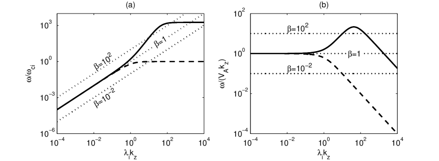
Figure 1: Wave frequency and phase velocity of the parallel right-hand circularly-polarized wave (solid lines), left-hand circularly-polarized wave (dashed lines), and ion acoustic wave (dotted lines) in the plasmas with $T_{i}=T_{e}$ but different $\beta$: $\beta=10^{-2}$, $1$ and $10^{2}$.

At the parallel propagation, the ion acoustic wave can interact with the right/left circularly-polarized waves at interaction points where their $\omega/\omega_{ci}$ and $\lambda_{i}k_{z}$ are equal as shown in Fig. (1). A mode transition can occur at the interaction point. The mode transition can happen among three oblique waves in Figs. (2)$-$(4). Also, Figs. (2)$-$(4) include the wave electromagnetic polarizations as well as the magnetic helicity $\sigma$ and the ion cross-helicity $\sigma_{Ci}$

$$\sigma=\frac{k\left(\mathbf{A\cdot\delta B^{\ast}}\right)}{\delta B^{2}}=\frac{2\mathrm{cos}\theta\left(i\delta B_{x}/\delta B_{y}\right)}{\mathrm{cos}^{2}\theta+\left(\delta B_{x}^{2}/\delta B_{y}^{2}\right)},$$

and

$$\sigma_{Ci}=\frac{2\mathrm{Re}\left(\delta\mathbf{v}_{i}\cdot\delta\mathbf{v}_{B}^{\ast}\right)}{\delta v_{i}^{2}+\delta v_{B}^{2}},$$

where $\mathbf{A}$ denotes the vector potential and $\delta v_{B}\equiv\delta B/\sqrt{\mu_{0}n_{0}m_{i}}$ is the magnetic field perturbation in the velocity unit.

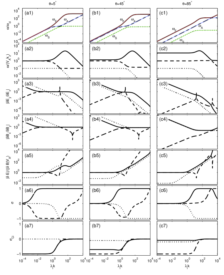
Figure 2: Wave dispersion relation and polarization at three propagating angles ($\theta=5^{\circ}$, $45^{\circ}$ and $85^{\circ}$) in the low-$\beta$ plasmas with $\beta=10^{-2}$ and $T_{e}=T_{i}$, where the solid, dashed and dotted lines denote the fast, Alfvén and slow modes, respectively. Thin solid lines in Panels (a1), (b1) and (c1) correspond to approximate dispersion relations (36) and (38) in the low-$\beta$ ($\beta\ll 1$) limit.

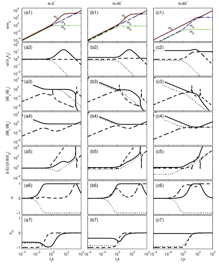
Figure 3: Wave dispersion relation and polarization at three propagating angles ($\theta=5^{\circ}$, $45^{\circ}$ and $85^{\circ}$) in $\beta=1$ plasmas with $T_{e}=T_{i}$, where the solid, dashed and dotted lines denote the fast, Alfvén and slow modes, respectively. Thin solid lines in Panels (a1), (b1) and (c1) correspond to the approximate dispersion relations (34) and (35).

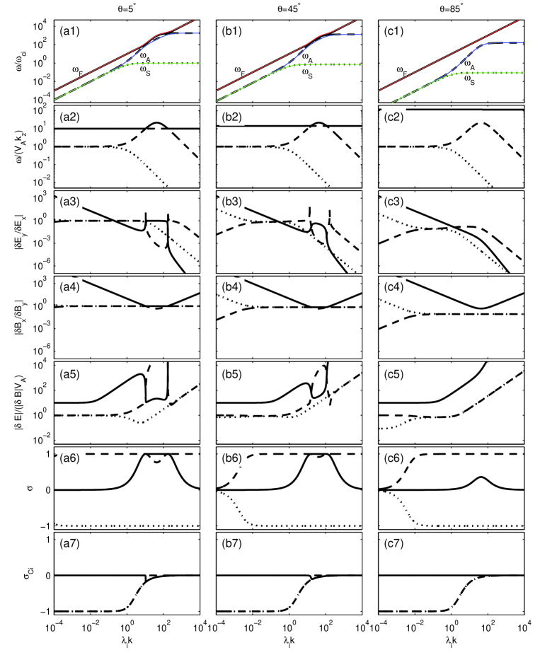
Figure 4: Wave dispersion relation and polarization at three propagating angles ($\theta=5^{\circ}$, $45^{\circ}$ and $85^{\circ}$) in the high-$\beta$ plasmas with $\beta=10^{2}$ and $T_{e}=T_{i}$, where the solid, dashed and dotted lines denote the fast, Alfvén and slow modes, respectively. Thin solid lines in Panels (a1), (b1) and (c1) represent the analytical dispersion relations (34) and (35) corresponding to the high-$\beta$ ($\beta\gg 1$) limit.

Fig. (2) presents the dispersion relations and polarizations of the three oblique waves at different angles in the low-$\beta$ plasmas where $\beta=10^{-2}$ and $T_{i}=T_{e}$. It shows that approximate dispersion relations (36) and (38) can describe the exact one (19) well.

The fast mode corresponds to the fast magnetosonic wave as $\omega\ll\omega_{ci}$ and the whistler wave as $\omega_{ci}\ll\omega\ll\left|\omega_{ce}\right|\cos\theta$. At the electron cyclotron frequency $\omega=\left|\omega_{ce}\right|\cos\theta$, the fast mode is the electron cyclotron wave. Furthermore, the electron cyclotron wave can change to a (quasi-) electroacoustic wave extending to higher frequency $\omega>\left|\omega_{ce}\right|\cos\theta$ fk69 . It is interesting to see that the fast magnetosonic wave has $\left(\left|\delta E_{y}/\delta E_{x}\right|,\left|\delta B_{x}/\delta B_{y}\right|\right)>1$ as $\lambda_{i}k<10^{-2}$, and $\left(\left|\delta E_{y}/\delta E_{x}\right|,\left|\delta B_{x}/\delta B_{y}\right|\right)\simeq 1$ as $10^{-2}<\lambda_{i}k\ll 1$ at the near-parallel propagation. $\left|\delta E/\delta B\right|\simeq V_{A}$ and $\sigma\simeq 0$ for the fast magnetosonic wave; $\left|\delta E/\delta B\right|>V_{A}$ and $\sigma\simeq 1$ for the whistler and electron cyclotron waves. In addition, $\sigma_{{Ci}}\simeq-\cos\theta$ for the fast magnetosonic wave kr94 , while $\sigma_{{Ci}}\simeq 0$ for the whistler and (quasi-) electroacoustic waves.

The Alfvén mode is the shear Alfvén wave at $\omega\ll\omega_{ci}$ and the (quasi-) electroacoustic wave at $\omega_{ci}<\omega<\left|\omega_{ce}\right|\cos\theta$ until a transition into the electron cyclotron wave at $\omega=\left|\omega_{ce}\right|\cos\theta$. At near-parallel $\theta=5^{\circ}$ and oblique $\theta=45^{\circ}$ cases, the phase velocity of the (quasi-) electroacoustic wave is about the sound speed. It is the Alfvén speed at the high oblique angle, therefore, Ref. zhao2014 called the high oblique mode at $\omega_{ci}<\omega<\left|\omega_{ce}\right|\cos\theta$ as the shear Alfvén wave. Note that an ion cyclotron wave $\omega\simeq\omega_{ci}$ arises at near-parallel propagation (Panel (a1)). Electromagnetic polarizations are $\left|\delta E_{x}\right|\gg\left|\delta E_{y}\right|$, $\left|\delta B_{y}\right|\gg\left|\delta B_{x}\right|$ and $\left|\delta E/\delta B\right|=V_{A}$ at $\omega\ll\omega_{ci}$; at $\omega_{ci}<\omega<\left|\omega_{ce}\right|\cos\theta$, $\left|\delta E/\delta B\right|$ becomes much larger than $V_{A}$. At $\theta=5^{\circ}$ and $45^{\circ}$, the magnetic-helicity $\sigma$ decreases firstly from $\sigma=0$ to $\sigma\simeq-1$ at $\omega\ll\omega_{ci}$, and then increases with increasing $\lambda_{i}k$ at $\omega_{ci}<\omega<\left|\omega_{ce}\right|\cos\theta$; at $\theta=85^{\circ}$, $\sigma=0$ is nearly unchanged at $\omega\ll\omega_{ci}$, and it becomes increasing at $\omega>\omega_{ci}$ until reaching $\sigma=1$ corresponding to the electron cyclotron wave. Besides, the ion cross helicity $\sigma_{{Ci}}$ depends on the wave scale, e.g., $\sigma_{Ci}=-1$ as $\lambda_{i}k\ll 1$ and $\sigma_{{Ci}}=0$ as $\lambda_{i}k\gg 1$.

The slow mode corresponds to the slow magnetosonic wave at $\omega\ll\omega_{ci}$, where $\left|\delta E_{x}\right|<\left|\delta E_{y}\right|$, $\left|\delta B_{x}\right|>\left|\delta B_{y}\right|$, $\left|\delta E/\delta B\right|\sim V_{T}$ and $\sigma=0$. It turns to the ion cyclotron wave at $\omega=\omega_{ci}\cos\theta$ bs03 , where $\left|\delta E_{x}\right|\gg\left|\delta E_{y}\right|$, $\left|\delta B_{x}\right|\sim\left|\delta B_{y}\right|$, $\left|\delta E/\delta B\right|>V_{A}$ and $\sigma=-1$. At $\theta=5^{\circ}$, the electric polarization $\left|\delta E_{y}/\delta E_{x}\right|$ has an increment at the transition position where the slow magnetosonic wave changes to the ion cyclotron wave; however, there is no such increment at $\theta=45^{\circ}$ and $\theta=85^{\circ}$ cases.

Figs. (3) and (4) present the dispersion relations and polarizations in $\beta=1$ and high-$\beta$ $\left(\beta=10^{2}\right)$ plasmas. Here the Alfvén mode interacts with the fast mode only. Although the validity condition for approximate dispersion relations (34) and (35) is $k_{\perp}^{2}/k_{z}^{2}>>1$ or $\beta\gg 1$, these expressions can describe the wave dispersion relations at $\beta=1$ as shown in Fig. (3).

Several mode properties in Fig. (3) are obviously different from that in the low-$\beta$ plasmas (Fig. (2)). For example, to the near-parallel waves at $0.1\omega_{ci}<\omega<\omega_{ci}$, two circularly polarized $\left(\left|\delta E_{x}\right|\simeq\left|\delta E_{y}\right|\right)$ modes are the fast and slow modes in $\beta=1$ plasmas but the fast and Alfvén modes in the low-$\beta$ plasmas. Here the fast (slow) mode exhibits the right-hand (left-hand) electric polarization and positive (negative) helicity. It also finds $\sigma\geq 0$ for the Alfvén mode in $\beta=1$ plasmas. Moreover, when the wave tends to more oblique propagation, the ion cross-helicity of the slow magnetosonic wave $\sigma_{{Ci}}\rightarrow-1$.

Fig. (4) shows that the Alfvén and slow modes are circularly polarized $\left(\left|\delta E_{x}\right|\simeq\left|\delta E_{y}\right|\right)$ waves at $\omega<\omega_{ci}$ in the high-$\beta$ plasmas, where the Alfvén (slow) mode exhibits the right-hand (left-hand) electric polarization and positive (negative) helicity. These two modes also have the same ion cross-helicity distribution. Note that three modes have no interaction point at the high oblique propagation as shown in Panel (c1).

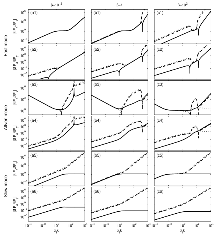
Figure 5: The sensitivity of the electric polarizations of the three modes on the temperature ratio $T_{e}/T_{i}$, where the waves propagate at $\theta=45^{\circ}$ in the plasmas with different $\beta$ environments: low-$\beta$ ($\beta=10^{-2}$), $\beta=1$, and high-$\beta$ ($\beta=10^{2}$). The solid, dashed and dotted lines represent the cold electron $T_{e}/T_{i}=0$, equal ion and electron temperature $T_{e}/T_{i}=1$, and cold ion $T_{e}/T_{i}=\infty$ cases, respectively.

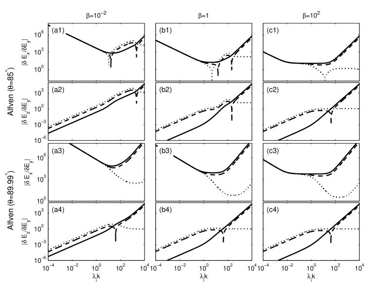
Figure 6: The dependence of the electric polarizations of high oblique Alfvén waves on the temperature ratio $T_{e}/T_{i}$, where two angles $\theta=85^{\circ}$ and $89.99^{\circ}$ are considered. The solid, dashed and dotted lines represent the cold electron $T_{e}/T_{i}=0$, equal ion and electron temperature $T_{e}/T_{i}=1$, and cold ion $T_{e}/T_{i}=\infty$ cases, respectively.

It needs to note that the electric field polarizations also strongly depend on the ratio of the electron to ion temperature $T_{e}/T_{i}$ (Eq. (23)). The electric field polarizations with different $T_{e}/T_{i}$ are presented in Fig. (5), where $\theta=45^{\circ}$ and $T_{e}/T_{i}=0$, $1$, and $\infty$. It shows that the parallel polarization $\left|\delta E_{z}/\delta E_{y}\right|$ decreases obviously with decreasing $T_{e}/T_{i}$. The transverse polarization $\left|\delta E_{x}/\delta E_{y}\right|$ is slightly affected by $T_{e}/T_{i}$ for the long-wavelength $\lambda_{e}k\ll 1$ waves, but not for the long-wavelength fast mode in the high-$\beta$ plasmas or for the long-wavelength slow mode in the low-$\beta$ plasmas. To understand qualitatively above results, the complete expressions Eq. (23) can reduce to

$$\frac{\delta E_{x}}{i\delta E_{y}} = -\frac{\widetilde{T}_{i}\omega^{2}V_{A}^{2}k^{2}+\widetilde{T}_{e}\left[\omega^{2}\left(\omega^{2}-V_{A}^{2}k_{z}^{2}\right)+V_{A}^{4}k^{2}k_{z}^{2}\right]}{\left(\omega^{2}-V_{A}^{2}k_{z}^{2}\right)\omega\omega_{ci}},$$

$$\frac{\delta E_{z}}{i\delta E_{y}} = -\frac{k_{z}}{k_{\perp}}\frac{\left(\omega^{2}+V_{A}^{2}k^{2}\right)}{\omega\omega_{ci}}\widetilde{T}_{e},$$ (32)

where the long-wavelength $\left(\lambda_{e}k\ll 1\right)$ and very low-frequency $\left(\Lambda_{1,2}\simeq 1\right)$ conditions are used, and the smaller terms of the order of $Q$ are neglected. Since $\widetilde{T}_{i}=1/\left(1+\gamma_{e}T_{e}/\gamma_{i}T_{i}\right)$ and $\widetilde{T}_{e}=\left(1-\widetilde{T}_{i}\right)$, $\left|\delta E_{z}/\left(i\delta E_{y}\right)\right|$ decreases with decreasing $T_{e}/T_{i}$. When $\omega\sim V_{A}k_{z}$, $\delta E_{x}/\left(i\delta E_{y}\right)\sim-V_{A}^{2}k^{2}\lambda_{i}k_{z}/\left(\omega^{2}-V_{A}^{2}k_{z}^{2}\right)$ is independent on $T_{e}/T_{i}$. We can also find $\delta E_{x}/\left(i\delta E_{y}\right)\sim-\widetilde{T}_{e}\omega/\omega_{ci}$ corresponding to the fast wave $\omega_{F}\sim V_{T}k$ in $\beta\gg 1$ plasmas and $\delta E_{x}/\left(i\delta E_{y}\right)\sim\widetilde{T}_{e}V_{A}^{2}k^{2}/\omega\omega_{ci}$ corresponding to the slow wave $\omega_{S}\sim V_{T}k_{z}$ in $\beta\ll 1$ plasmas, which indicate $\left|\delta E_{x}/\left(i\delta E_{y}\right)\right|$ decreasing with smaller $T_{e}/T_{i}$. Besides, in Fig. (5) the electric polarizations $\left|\delta E_{x}/\delta E_{y}\right|$ and $\left|\delta E_{z}/\delta E_{y}\right|$ in $T_{e}/T_{i}\neq 0$ plasmas increase continuously as the slow magnetosonic wave changes to the ion cyclotron wave, while both polarizations are nearly unchanged in $T_{e}/T_{i}=0$ plasmas. Note that the main characters in Fig. (5) still appear in the electric polarization distributions of the oblique waves with $\theta\neq 45^{\circ}$.

When the phase relation of the electric polarizations changes, a peak or a valley can occur in $\left|\delta E_{x}/\delta E_{y}\right|$ and $\left|\delta E_{z}/\delta E_{y}\right|$ distributions. For the fast mode in Fig. (5), the phase relation of $\delta E_{z}/\delta E_{y}$ changes in $T_{e}/T_{i}=0$ plasmas, while it is unchanged in $T_{e}/T_{i}\neq 0$ plasmas. For the Alfvén mode, two transition points arise in the phase relation of $\delta E_{x}/\delta E_{y}$ in $T_{e}/T_{i}\neq 0$ plasmas; however, in the cold electron $\left(T_{e}/T_{i}=0\right)$ plasmas, the transition at the smaller $\lambda_{i}k$ disappears in $\beta\ll 1$ plasmas, or two transitions are both missing in $\beta\geq 1$ plasmas.

For near-perpendicular Alfvén wave, Fig. (6) shows that the parallel polarization $\left|\delta E_{z}/\delta E_{y}\right|$ increases (decreases) with $T_{e}/T_{i}$ as $\lambda_{i}k<10^{2}$ $\left(\lambda_{i}k>10^{2}\right)$. At $\theta=89.99^{\circ}$, the transverse polarization $\left|\delta E_{x}/\delta E_{y}\right|$ decreases with increasing $T_{e}/T_{i}$ for the kinetic-scale Alfvén waves $\left(\lambda_{i}k>1\right)$. These results indicate the important role of the electron temperature $T_{e}$ on the kinetic-scale Alfvén waves le99 ; ya14 . Moreover, there is no transition of the phase relation of $\delta E_{x}/\delta E_{y}$ at $\theta=89.99^{\circ}$ case. The reason is that the wave frequency $\omega$ is smaller than the ion cyclotron frequency $\omega_{ci}$ at $\theta=89.99^{\circ}$, which cannot satisfy the frequency condition $\omega>\omega_{ci}$ for the changing of the phase relation of transverse electric polarization zhao2014 .

IV Summary

In this study ions and electrons are treated separately in comparison with one fluid element $\left(U=\sum m_{\alpha}v_{\alpha}/\sum m_{\alpha}\right)$ method adopted in previous studies st63 ; be12 . This method is helpful to obtain the linear eigenfunctions including the ion and electron velocities as well as the ion and electron cross-helicities.

It found that the fast and Alfvén modes are nearly linearly polarized at the very low-frequency $\omega\ll 10^{-2}\omega_{ci}$, and circularly polarized at $10^{-2}\omega_{ci}<\omega<\omega_{ci}$ at the near-parallel propagation in the low-$\beta$ plasmas. Two circularly polarized modes become the fast and slow modes in a narrow frequency regime $0.1\omega_{ci}<\omega<\omega_{ci}$ in $\beta=1$ plasmas; they are the Alfvén and slow modes in $\beta=10^{2}$ plasmas. To the ion cross-helicity $\sigma_{{Ci}}$ of the long-wavelength slow mode, $\sigma_{{Ci}}\simeq 0$ in the low-$\beta$ plasmas, $\sigma_{{Ci}}\rightarrow-1$ as $\theta\rightarrow 90^{\circ}$ in $\beta=1$ plasmas, and $\sigma_{{Ci}}\simeq-1$ in the high-$\beta$ plasmas. It also found that the negative magnetic-helicity $\sigma$ of the Alfvén mode can occur at the small or moderate angles in the low-$\beta$ plasmas, while $\sigma\geq 0$ arises always at the high oblique angle in the low-$\beta$ plasmas or at the general angle in $\beta\geq 1$ plasmas.

Our results exhibited the sensitivity of the electric polarizations on the temperature ratio $T_{e}/T_{i}$. The parallel polarization $\left|\delta E_{z}/\delta E_{y}\right|$ decreases with $T_{e}/T_{i}$ as $\lambda_{i}k<1$. The transverse polarizations $\left|\delta E_{x}/\delta E_{y}\right|$ also decreases with $T_{e}/T_{i}$ for the long-wavelength fast mode in the high-$\beta$ plasmas, or for the long-wavelength slow mode in the low-$\beta$ plasmas, while $\left|\delta E_{x}/\delta E_{y}\right|$ at other long-wavelength cases are slightly affected by $T_{e}/T_{i}$. Furthermore, the phase relation of $\delta E_{x}/\delta E_{y}$ of the Alfvén mode will change in $T_{e}/T_{i}\neq 0$ plasmas, but this change can disappear in the cold electron $T_{e}/T_{i}=0$ plasmas. For the fast mode, the phase relation of $\delta E_{z}/\delta E_{y}$ changes in $T_{e}/T_{i}=0$ plasmas, while the unchanged phase relation arises in $T_{e}/T_{i}\neq 0$ plasmas.

We have also presented the approximate dispersion relations in the near-perpendicular propagation, low-$\beta$, and high-$\beta$ limits. These approximations can describe nicely the exact dispersion relations of the three modes given by Eq. (19). It notes that the condition of $V_{A}^{2}/c^{2}\ll 1$ used in the study leads to the neglecting of the displacement current. However, this assumption is broken near the wave cutoff position which results in the validity condition of $\omega\ll\omega_{ci}\left(1+c^{2}/V_{A}^{2}\right)$ be12 . Also, the displacement current may be important in producing the parallel electric field of the low-frequency Alfvén mode sl06 . Therefore, a comprehensive study including the effect of the displacement current is needed.

Lastly, two-fluid model neglects the kinetic wave-particle interaction effects, such as Landau damping and ion (electron) cyclotron resonance damping, which can only be captured by the kinetic model. These kinetic effects can strongly affect the wave dispersion relation and polarization properties. For example, the wave dispersion relation of the kinetic Alfvén wave is depressed at ion scales in the high-$\beta$ plasmas where there can be the heavy Landau damping ho06 . The two models also result in different phase relation between two electric components. However, since it is difficult to identify clearly all modes from the full kinetic theory, the two-fluid theory can be a useful guide to discard the modes in the kinetic theory. Our complete expressions can be conveniently used to compare with the results of the kinetic model.

Appendix A Approximate dispersion relations in different limits

A.1 Near-perpendicular propagation limit

At the near-perpendicular propagation limit $k_{z}^{2}/k_{\perp}^{2}\ll 1$, the cubic equation (18) for $\omega^{2}$ can reduce to a quadratic equation

$$A_{\mathrm{obli}}\omega^{4}-B_{\mathrm{obli}}\omega^{2}+C_{\mathrm{obli}}=0,$$ (33)

where

$$A_{\mathrm{obli}} = 1+\lambda_{e}^{2}k^{2}+\lambda_{i}^{2}k_{z}^{2}+\left(1+\lambda_{e}^{2}k^{2}\right)^{2}\beta+k_{z}^{2}/k^{2},$$

$$B_{\mathrm{obli}} = \left(1+2\beta+\rho^{2}k^{2}\right)V_{A}^{2}k_{z}^{2},$$

$$C_{\mathrm{obli}} = \beta V_{A}^{4}k_{z}^{4},$$

which contains the dispersion relation of the Alfvén mode $\left(\omega_{A}=\omega_{+}\right)$ and slow mode $\left(\omega_{S}=\omega_{-}\right)$,

$$\omega_{\pm}^{2} = V_{A}^{2}k_{z}^{2}\frac{1+2\beta+\rho^{2}k^{2}}{2\left(1+\lambda_{e}^{2}k^{2}+\lambda_{i}^{2}k_{z}^{2}+\left(1+\lambda_{e}^{2}k^{2}\right)^{2}\beta+k_{z}^{2}/k^{2}\right)}$$ (34)

$$\left[1\pm\sqrt{1-4\beta\frac{1+\lambda_{e}^{2}k^{2}+\lambda_{i}^{2}k_{z}^{2}+\left(1+\lambda_{e}^{2}k^{2}\right)^{2}\beta+k_{z}^{2}/k^{2}}{\left(1+2\beta+\rho^{2}k^{2}\right)^{2}}}\right]$$

On the other hand, the fast mode can be obtained by first two terms in Eq. (18),

$$\omega_{F}=V_{A}k\frac{\sqrt{1+\lambda_{e}^{2}k^{2}+\lambda_{i}^{2}k_{z}^{2}+\left(1+\lambda_{e}^{2}k^{2}\right)^{2}\beta+k_{z}^{2}/k^{2}}}{1+\lambda_{e}^{2}k^{2}}.$$ (35)

A.2 Low-$\beta$ $\left(\beta\ll 1\right)$ limit

In low-$\beta$ plasmas with $\beta\ll 1$, the frequency of the slow mode $\omega_{S}\sim V_{T}k_{z}$ is much smaller than that of the fast mode $\omega_{F}\sim V_{A}k$ and Alfvén mode $\omega_{A}\sim V_{A}k_{z}$. So that the last two terms in Eq. (18) control the dispersion relation of the slow mode

$$\omega_{S}=\frac{V_{T}k_{z}}{\sqrt{1+\rho^{2}k^{2}}}.$$ (36)

On the other hand, the fast and Alfvén modes are controlled by following quadratic equation

$$A_{\mathrm{low}}\omega^{4}-B_{\mathrm{low}}\omega^{2}+C_{\mathrm{low}}=0,$$ (37)

where

$$A_{\mathrm{low}} = \left(1+\lambda_{e}^{2}k^{2}\right)^{2},$$

$$B_{\mathrm{low}} = \left(1+\lambda_{e}^{2}k^{2}+\left(1+\lambda_{e}^{2}k^{2}\right)^{2}\beta+\lambda_{i}^{2}k_{z}^{2}+k_{z}^{2}/k^{2}\right)V_{A}^{2}k^{2},$$

$$C_{\mathrm{low}} = \left(1+\rho^{2}k^{2}\right)V_{A}^{4}k^{2}k_{z}^{2},$$

which yields the dispersion relations for the fast mode $\left(\omega_{F}=\omega_{+}\right)$ and Alfvén mode $\left(\omega_{A}=\omega_{-}\right)$

$$\omega_{\pm}^{2} = V_{A}^{2}k^{2}\frac{1+\lambda_{e}^{2}k^{2}+\left(1+\lambda_{e}^{2}k^{2}\right)^{2}\beta+\lambda_{i}^{2}k_{z}^{2}+k_{z}^{2}/k^{2}}{2\left(1+\lambda_{e}^{2}k^{2}\right)^{2}}$$ (38)

$$\left[1\pm\sqrt{1-\frac{4\left(1+\lambda_{e}^{2}k^{2}\right)^{2}\left(1+\rho^{2}k^{2}\right)}{\left(1+\lambda_{e}^{2}k^{2}+\left(1+\lambda_{e}^{2}k^{2}\right)^{2}\beta+\lambda_{i}^{2}k_{z}^{2}+k_{z}^{2}/k^{2}\right)^{2}}\frac{k_{z}^{2}}{k^{2}}}\right].$$

A.3 High-$\beta$ $\left(\beta\gg 1\right)$ limit

In high-$\beta$ plasmas with $\beta\gg 1$, the frequency of the fast mode $\omega_{F}\sim V_{T}k$ is much larger than that of the Alfvén and slow modes $\omega_{A,S}\sim V_{A}k_{z}$. The fast mode are dominant by the first two terms in Eq. (18), whereas the Alfvén and slow modes are dominant by the quadratic equation shown in Eq. (33). Therefore, the wave dispersion relations of the three modes are the same as that given by Eqs. (34) and (35).

References

(1) T. E. Stringer, J. Nucl. Energy, Part C 5, 89 (1963).
(2) V. Formisano, and C. F. Kennel, J. Plasma Phys. 3,
55 (1969).
(3) D. G. Swanson, Plasma Waves (Academic, London, 1989).
(4) A. Ishida, C. Z. Cheng, and Y-K. M. Peng, Phys. Plasmas,
12, 052113 (2005).
(5) P. A. Damiano, A. N. Wright, and J. F. McKenzie, Phys.
Plasmas, 16, 062901 (2009)
(6) D. Krauss-Varban, N. Omidi, and K. B. Quest, J. Geophys.
Res., 99, 5987 (1994).
(7) P. M. Bellan, J. Geophys. Res., 117, A12219 (2012).
(8) J. V. Hollweg, J. Geophys. Res. 104, 14811 (1999).
(9) P. K. Shukla, and L. Stenflo, J. Plasma Phys. 64,
125 (2000).
(10) L. Chen, and D. J. Wu, Phys. Plasmas 18, 072110
(2011).
(11) J. S. Zhao, Y. Voitenko, M. Y. Yu, J. Y. Lu and J. D. Wu,
Astrophys. J. 793, 107 (2014).
(12) T. J. M. Boyd and J. J. Sanderson, The Physics of
Plasmas (Cambridge University Press, New York, 2003).
(13) T. H. Stix, The Theory of Plasma Waves (McGraw-Hill,
New York, 1992).
(14) D. Verscharen, and B. D. G. Chandran, Astrophys. J. 764, 88,
(2013).
(15) R. J. Leamon, C. W. Smith, N. F. Ness, and H. K. Wong, J.
Geophys. Res., 104, 22331, (1999).
(16) Y. Song, and L. Lysak, Phys. Rev. Lett. 96, 145002 (2006).
(17) L. Yang, D. J. Wu, S. J. Wang, and L. C. Lee, Astrophys. J.
792, 36, (2014).
(18) G. G. Howes, S. C. Cowley, W. Dorland, G. W. Hammett, E.
Quataert, and A. A. Schekochihin, Astrophys. J. 651, 590 (2006).