Classification of Majorana Fermions in Two-Dimensional Topological Superconductors

Abstract

Recently, Majorana Fermions (MFs) have attracted intensive attention due to their exotic statistics and possible applications in topological quantum computation (TQC). They are proposed to exist in various two-dimensional (2D) topological systems, such as $p_{x}+ip_{y}$ topological superconductor and nanowire-superconducting hybridization system. In this paper, two types of Majorana Fermions with different polygon sign rules are pointed out. A “smoking gun” numerical evidence to identify MF’s classification is presented through looking for the signature of a first order topological quantum phase transition. By using it, several 2D topological superconductors are studied.

I Introduction

Majorana fermion is a real fermion that is its own antiparticleMajorana ; Wilczek ; Martin . Because of its exotic properties and the possible exotic statisticsKitaev01 ; Fu08 ; Lutchyn10 ; Oreg10 ; Sau10 ; Alicea10 ; Potter10 ; Alicea11 ; Halperin12 ; Stanescu13 ; Mourik12 ; Das12 ; Deng12 ; Rokhinson12 ; Churchill13 , in condensed matter physics, the search for Majorana fermions (MFs) has attracted increasing interests. A variety of schemes to realize MFs (more accurately, Majorana bound states) have been proposed. A possible approach is to create a quantized vortex ($\pi$-flux) in the $p_{x}+ip_{y}$-wave topological superconductors (SC) that traps MFs in vortex-coreMoore91 ; Read00 ; Ivanov01 ; Nayak08 ; Alicea12 . Then, it is known that the quantized vortex in two dimensional (2D) topological SC with nonzero Chern number hosts a MF with exact zero energy. Another different approach to realize MFs is to consider a one-dimensional (1D) electronic nano-structures proximity-coupled to a bulk superconductorKitaev01 , of which the unpaired Majorana fermions appear as the end-states. Then, based on this idea, several schemes are proposed to realize MFs that appear as the end-states of line-defects in 2D non-topological SCskou .

To describe the Majorana zero mode, a real fermion field called Majorana fermion $\gamma=\int d{r}[u_{0}\psi^{\ast}+v_{0}\psi]$ ($\gamma^{\dagger}=\gamma$) is introduced. We consider a 2D gapped SC with a pair of Majorana modes with nearly zero energies, of which the corresponding MFs are denoted by $(\gamma_{1},$ $\gamma_{2})$. To describe the subspace of the system with two nearly degenerate states, the Fermion-parity operator $\mathrm{\hat{P}}=-i\gamma_{1}\gamma_{2}$ is introduced. Since $\mathrm{\hat{P}}^{2}=1$, $\mathrm{\hat{P}}$ has two eigenvalues $\pm 1,$ called even and odd Fermion-parities, respectively. Generally, there exists the coupling between two MFs and the effective Hamiltonian is given by $it\gamma_{1}\gamma_{2}$ where $t$ is the coupling constant. The quantum systems with multi-MFs (we call this lattice model to be Majorana lattice model) show nontrivial topological properties, including a nonvanishing Chern number, chiral Majorana edge stateVILL ; kou2 ; kou1 . It was pointed out that the Majorana lattice model is really an induced ”topological superconductor” on the parent TSC.

A question arises, ”Do MFs in different topological superconductors belong to the same class?” Without no detectable degree of freedoms (MFs have zero energy, zero charge, zero spin), it is believed that MFs have ”no Hair”. Therefore, it was believed that all MFs in different models are same and belong to the same class. In this paper we point out that in 2D topological systems, MFs do have ”hair”, that is the number of quantized vortex, a topological degree of freedom. As a result, there exist two universal classes of MFs: MFs binding a $\pi$-flux and those with no flux-binding. We then introduce a topological value to characterize the two classes of MFs and propose an (indirect) numerical approach to identify the class of MFs in topological systems. Our basis is the fact that multi-MFs with $\pi$-flux may be topologically different from those with no flux-binding in the Fermion-parity of the ground states and the order of quantum phase transitions. By calculating a dimensionless parameter, the gap ratio (see discussion below), the quantum number of the MFs becomes an observable ”quantity”.

II Classification of Majorana fermions

We begin by giving the definitions of two classes of MFs in 2D topological systems. One class contains the usual MFs without flux-binding (we call this class normal MFs); the other class contains composite objects of an MF together with a $\pi$-flux (we call this class topological MFs). See the illustrations of the two classes of MFs in Fig.1.(a) and Fig.3.(a).

We consider a system with coupled MFs. The coupling strength is just the energy splitting from the intervortex quantum tunneling. We call this effective description as the Majorana lattice model, of which the tight-binding Hamiltonian can be written as

$$\mathcal{H}_{m.f}=i\sum_{(j,k)}s_{jk}t_{jk}\gamma_{k}\gamma_{j}$$ (1)

where $t_{jk}$ is the hopping amplitude from $j$ to $k$, and satisfies $t_{jk}=t_{jk}^{\ast}$. $\gamma_{j}$ is a Majorana operator ($\gamma_{j}^{{\dagger}}=\gamma_{j}$) obeying anti-commutate relation $\{\gamma_{j},\gamma_{k}\}=2\delta_{jk}$. $s_{ij}=-s_{ji}$ is a gauge factor. Thus, the total number of Majorana modes $N$ must be even and then we can divide the Majorana lattice into two sublattices. The pair $(j,k)$ denotes the summation that runs over all the nearest neighbor (NN) pairs (with hopping amplitude $t$) and all the next-nearest neighbor (NNN) pairs (with hopping amplitude $t^{\prime}$). Each triangular plaquette possesses $\pm\pi/2$ quantum flux effectively.

This Hamiltonian allows different $Z_{2}$ gauge choices (sign rules) $s_{jk}=\pm 1$. From the theory of projective symmetry group, there are two possible gauge choices (sign rules) that correspond to two different classes of MFs: topological MFs obey a topological polygon sign rule; normal MFs obey a normal polygon sign rule. According to topological polygon sign rule for topological MFs, there exists an extra phase related to a closed path that forms a polygon, given by half the sum of the interior angles of the polygonEGR . Thus, for $4N$ ($4N\pm 1$) topological MFs on a ring, there exists $\pm\pi$ ($\pm\pi/2$) flux inside the ring; for $4N\pm 2$ topological MFs on a ring, there is no flux inside the ring. On the contrary, according to normal polygon sign rule for normal MFs, there also exists an extra phase related to a closed path that forms a polygon. However, for $4N\pm 1$ normal MFs on a ring, there exists $\pm\pi/2$ flux inside the ring and for $4N$ or $4N\pm 2$ normal MFs on a ring, there is no flux inside the ring.

III Quantum phase transitions in dimerized Majorana rings

III.1 The Hamiltonian of Majorana rings

We begin from a (dimerized) Majorana ring of $4N$ MFs ($N$ is a positive integer number). The Hamiltonian readsKitaev01

$$\mathcal{\hat{H}}_{\mathrm{MF}} =i\sum_{j=1}^{2N-\delta_{1,N}}(J_{1}^{\prime}\gamma_{jb}\gamma_{j+1,a}+J_{1}\gamma_{ja}\gamma_{jb}$$ (2)

$$+J_{2}\gamma_{jb}\gamma_{j+1,b}+J_{2}\gamma_{ja}\gamma_{j+1,a})$$

where $a$, $b$ denote the sublattices in a unit cell, $J_{1}$ is the coupling constants between two MFs in a unit cell, $J_{1}^{\prime}$ ($J_{2}$) are the (next) nearest coupling constants between two MFs in different unit cells. For the case of $N=1$, $\delta_{1,N}=1;$ For the case of $N>1$, $\delta_{1,N}=0$. For usual systems, we have $J_{2}<J_{1},$ $J_{1}^{\prime}$.

For a Majorana ring with $4N$ normal MFs (we call it normal Majorana ring), due to normal polygon sign rule, we always have periodic boundary condition; while for a Majorana ring with $4N$ topological MFs (we call it topological Majorana ring), due to topological polygon sign rule, we have anti-periodic boundary condition owing to an extra $\pi$ flux inside the ring. Fig.1.(a) and Fig.3.(a) illustrate a Majorana ring with $8$ normal MFs and that with $8$ topological MFs, respectively.

III.2 Quantum phase transitions in normal Majorana rings

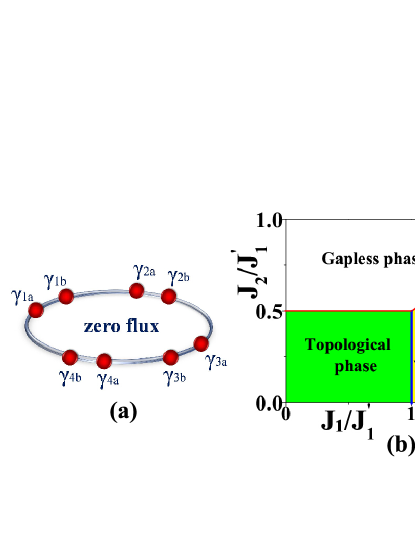
Figure 1: (color online) (a) Illustration of an normal Majorana ring with 8 normal Majorana Fermions (red dots); (b) Phase diagram of normal Majorana ring in thermodynamic limit, $N\rightarrow\infty$. The blue line denotes the first order topological quantum phase transition that switches Fermion-parity of the ground state and the red lines denote the second order phase transitions.

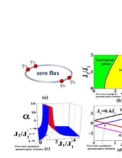
Figure 2: (color online) (a) Illustration of the normal Majorana ring with four Majorana Fermions; (b) Phase diagram of the normal Majorana ring with four Majorana Fermions. The blue line denotes the first order topological quantum phase transition that switches Fermion-parity of the ground state; (c) The gap-ratio of the normal Majorana ring with four Majorana Fermions. The divergence of the gap-ratio, $\alpha\rightarrow\infty,$ denotes a first order topological quantum phase transition; (d) The energy levels of the normal Majorana ring with four Majorana Fermions at $J_{2}=0.4J_{1}^{\prime}$. The level-crossing denotes a first order topological quantum phase transition.

Firstly, we study a (dimerized) Majorana ring with $4N$ normal MFs. We pair ($\gamma_{ja}$, $\gamma_{jb}$) into a complex fermion as $\gamma_{ja}=(c_{j}+c_{j}^{{\dagger}})/\sqrt{2},$ $\gamma_{jb}=-i(c_{j}-c_{j}^{{\dagger}})/\sqrt{2},$ where $c_{j}$ ($c_{j}^{{\dagger}}$) annihilates (creates) a complex fermion. Then the Majorana ring’s energy spectra can be obtained through a fourier transformation $c_{k}=N^{-1/2}\sum_{i}e^{-ikR_{i}}c_{i}$. In thermodynamic limit, $N\rightarrow\infty$, the Hamiltonian in momentum space takes the form of

$$\mathcal{\hat{H}}_{\mathrm{MF}} =\sum_{k}\psi_{k}^{{\dagger}}[(-J_{1}^{\prime}\cos k+J_{1})\tau^{z}$$ (3)

$$+(J_{1}^{\prime}\tau^{y}-2J_{2})\sin k]\psi_{k}$$

where $\psi_{k}^{{\dagger}}=(c_{k}^{{\dagger}},c_{-k})$ and $\tau^{z},$ $\tau^{y}$ are Pauli matrices. The energy spectra are given by

$$E_{\pm}(k)=-2J_{2}\sin k\pm\sqrt{(J_{1}^{\prime})^{2}-2J_{1}^{\prime}J_{1}\cos k+J_{1}^{2}}$$ (4)

where $k=\pi n/N,$ $n=1,2,...,2N.$

To characterize the topological properties of the ground states, we define a Fermion-parity operator in the following form

$$\mathrm{\hat{P}}=\prod_{j=1}^{2N}(-i\gamma_{ja}\gamma_{jb}).$$ (5)

Since $\mathrm{\hat{P}}^{2}=1$, $\mathrm{\hat{P}}$ has two eigenvalues $\pm 1,$ called even and odd Fermion-parities, respectively. Due to $[\mathrm{\hat{P}},$ $\mathcal{\hat{H}}_{\mathrm{MF}}]=0$, the ground state $\left|vac\right\rangle$ should have a determinant parity $\mathrm{\hat{P}}\left|vac\right\rangle=\pm\left|vac\right\rangle$. For the case of $\mathrm{\hat{P}}\left|vac\right\rangle=-\left|vac\right\rangle,$ the ground state is a topological phase; for the case of $\mathrm{\hat{P}}\left|vac\right\rangle=\left|vac\right\rangle,$ the ground state is a non-topological phase.

For the Majorana ring described by Eq.(2), the eigenvalues of $\mathrm{\hat{P}}$ is equal to

$$\mathrm{sgn}(E(k=0)\cdot E(k=\pi))$$ (6)

  where $E(k=0)=J_{1}-J_{1}^{{}^{\prime}}$ at $k=0$ and $E(k=\pi)=J_{1}+J_{1}^{{}^{\prime}}$ at $k=\pi.$ Thus, at $J_{1}=J_{1}^{{}^{\prime}}$, the energy gap closes, $E_{\pm}(k)=0,$ at which a topological quantum phase transition (TQPT) occursKitaev01 . In Fig.1.(b), we plot the global phase diagram of the normal Majorana ring in thermodynamic limit, $N\rightarrow\infty$. There are three phases: gapless phase (we don’t discuss this phase due to triviality), topological phase and non-topological phase. The blue line denotes the first order TQPT that switches the Fermion-parity of the ground stateKitaev01 and the red lines denote the second order phase transitions. In yellow region ($J_{1}>J_{1}^{{}^{\prime}}$, $J_{2}<J_{1}$), we have $\mathrm{P}=1$ and the ground state corresponds to a trivial state (non-topological phase) with even Fermion-parity, $\mathrm{\hat{P}}\left|vac\right\rangle=\left|vac\right\rangle$. In green region ($J_{1}<J_{1}^{{}^{\prime}},$ $J_{2}<J_{1}^{\prime}$), we have $\mathrm{P}=-1$ and the ground state corresponds to a topological phase with odd Fermion-parity, $\mathrm{\hat{P}}\left|vac\right\rangle=-\left|vac\right\rangle$kou3 . So, for a normal Majorana ring with arbitrary $N,$ a first order TQPT that switches the Fermion-parity occurs at $J_{1}=J_{1}^{{}^{\prime}}$.

On the other hand, for a Majorana ring with 4 normal MFs (or $N=1$), the phase diagram (See Fig.2.(b)) differs from the case in thermodynamic limit (or $N\rightarrow\infty$) (See Fig.1.(b)). The blue line in Fig.2.(b) denotes the first order TQPT that switches the fermion-parity of the ground state. To make the TQPT in a Majorana ring with only 4 MFs more clear, we plot the energy levels for the case $J_{2}=0.4J_{1}^{\prime}$ in Fig.2.(d). Now, the four energy levels are $E_{\pm}(k=0),$ $E_{\pm}(k=\pi).$ The level-crossing in Fig.2.(d) shows the first order TQPT corresponding to the blue line in Fig.2.(b)).

In addition, to characterize the TQPT, we introduce a dimensionless parameter - gap-ratio,

$$\alpha=\frac{\max\left|E_{k}\right|-\min\left|E_{k}\right|}{\min\left|E_{k}\right|}$$ (7)

where $\max\left|E_{k}\right|$ and $\min\left|E_{k}\right|$ are the maximum value and minimum value of the energy levels of the multi-MFs, respectively. When the gap-ratio turns to infinite, the energy gap closes and TQPT occurs. In the thermodynamic limit, the gap-ratio $\alpha$ becomes $\frac{W_{\mathrm{MF}}}{\Delta_{\mathrm{MF}}}$ where $W_{\mathrm{MF}}=\max\left|E_{k}\right|-\min\left|E_{k}\right|$ is the band-width and $\Delta_{\mathrm{MF}}=\min\left|E_{k}\right|$ is the energy gap of the Majorana ring. This is why we call $\alpha$ gap-ratio. On the other hand, for an normal Majorana ring with four MFs (or $N=1$), due to $\max\left|E_{k}\right|=\left|E(k=\pi)\right|$ and $\min\left|E_{k}\right|=\left|E(k=0)\right|$, the gap-ratio $\alpha$ is equal to $\left|\frac{E(k=\pi)}{E(k=0)}\right|-1.$ In particular, at TQPT, accompanied by gap-closing, $\Delta_{\mathrm{MF}}=0$ or $E(k=0)=0$, the gap-ratio diverges,

$$\alpha\rightarrow\infty.$$ (8)

See the results in Fig.2.(c).

III.3 Quantum phase transitions in topological Majorana rings

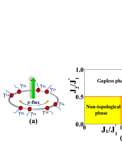
Figure 3: (color online) Illustration of a topological Majorana ring with 8 topological Majorana Fermions (red dots with strings). Due to the polygon rule, there exists an extra $\pi$-flux inside the ring for topological Fermions; (b) Phase diagram of topological Majorana ring in thermodynamic limit, $N\rightarrow\infty$. The red lines denote the second order phase transitions.

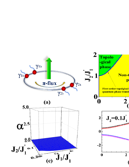
Figure 4: (color online) (a) Illustration of the topological Majorana ring with four Majorana Fermions. Due to the polygon rule, there exists an extra $\pi$-flux inside the ring for topological Majorana Fermions; (b) Phase diagram of the topological Majorana ring with four Majorana Fermions. The blue line denotes the first order topological quantum phase transition that switches Fermion-parity of the ground state; (c) The gap-ratio of the topological Majorana ring with four Majorana Fermions; (d) The energy levels of the topological Majorana ring with four Majorana Fermions at $J_{2}=0.1J_{1}^{\prime}$.

Next, we study a (dimerized) Majorana ring of $4N$ topological MFs. Due to the extra $\pi$-flux inside the ring, we have an anti-periodic boundary condition of the topological Majorana ring. The energy spectra are the same to those of the normal Majorana ring as

$$E_{\pm}(k)=-2J_{2}\sin k\pm\sqrt{(J_{1}^{\prime})^{2}-2J_{1}^{\prime}J_{1}\cos k+J_{1}^{2}}$$ (9)

with different wave-vectors, $k=\pi(n-1/2)/N,$ $n=1,2,...,2N.$ Now, there are no high symmetry points at $k=0,$ $k=\pi$. As a result, the ground state always has even fermion-parity, $\mathrm{\hat{P}}\left|vac\right\rangle\equiv\left|vac\right\rangle$. In thermodynamic limit, a second order phase transition occurs at $J_{1}=J_{1}^{{}^{\prime}}$ between a non-topological phase (the left yellow region in Fig.3.(b)) and another non-topological phase (the right yellow region in Fig.3.(b)). For the topological Majorana rings with finite $N$, the energy levels can smoothly change from one phase to the other without level-crossing. At the quantum critical point, $J_{1}=J_{1}^{{}^{\prime}}$, in the thermodynamic limit, we have $\alpha\sim N\rightarrow\infty$; while for finite $N$, $\alpha$ is a finite value.

On the other hand, for a Majorana ring with 4 topological MFs (or $N=1$), the phase diagram differs from that for the normal case. See the results in Fig.4.(b). A first order TQPT occurs in the region with large $J_{2}$ that is irrelevant to traditional topological systems. In the region with small $J_{2}$, the first order TQPT will never occur. In Fig.4.(c), the four energy levels for a topological Majorana ring with four MFs are $E_{\pm}(k=\pi/2),$ $E_{\pm}(k=-\pi/2).$ In Fig.4.(d), the energy levels of the topological Majorana ring with four Majorana Fermions are plotted for the case of $J_{2}=0.1J_{1}^{\prime}$. The gap-ratio for topological MFs is obtained to be

$$\alpha=\left|\frac{E_{+}(k=-\pi/2)}{E_{+}(k=\pi/2)}\right|-1.$$

For the case of $J_{2}\ll J_{1},$ $J_{1}^{\prime}$, due to $E_{\pm}(k=\pi/2)\simeq E_{\pm}(k=-\pi/2)$, we always have a very small gap-ratio as

$$\alpha\rightarrow 0.$$ (10)

IV Numerical Method to identify the Majorana Fermion’s classification

From above discussion, the sharp distinctions between normal and topological MFs are found in relevant physics ($J_{2}<J_{1},$ $J_{2}<J_{1}^{\prime}$): for four normal MFs on a ring, at the point of first order TQPT, $\alpha\rightarrow\infty$ (or $\alpha\gg 1$); for four topological MFs on a ring, without the first order TQPT, $\alpha\rightarrow 0$ (or $\alpha<1$). Therefore, we propose a numerical method to distinguish the normal/non-normal polygon sign rule for the MFs by calculating the gap-ratio $\alpha$ in a topological system with four MFs that form a (dimerized) Majorana ring.

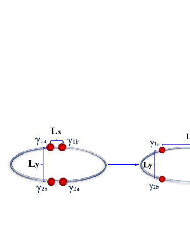
Figure 5: (color online) Illustration of the varying of a Majorana ring with four Majorana Fermions from the limit $L_{x}/L_{y}\ll 1$ (or $J_{1}/J_{1}^{{}^{\prime}}\gg 1$) to the limit $L_{x}/L_{y}\gg 1$ (or $J_{1}/J_{1}^{{}^{\prime}}\ll 1$).

In the first step, we study the given 2D topological system without considering the MFs. After diagonalizing the BdG equation, we obtain the energy spectra in momentum space $E(\mathbf{k})$ and the energy gap of the system $\Delta_{f}$.

In the second step, the energy levels of the 2D topological system with a pair of MFs ($\gamma_{1}$, $\gamma_{2}$) are calculated by numerical approach. We can derive the energy levels of the MFs with almost zero energies, $\pm E$, ($E>0$). When there are two MFs nearby, the quantum tunneling effect occurs and the two MFs couple. The energy splitting between two nearly zero modes $\Delta E=2E$ versus the distance $L$ of the two MFs can be obtained. In general, $\Delta E$ oscillates and decreases exponentially with $L$ and can be described by a function as $\Delta E\propto e^{-L/\xi}\left|\cos(L\cdot k_{F})\right|$ where $\xi\sim v_{F}/\Delta_{f}$ is the correlated length $\xi$ and $v_{F}$ is the Fermi velocity. We plot the enveloping line of $\Delta E$ (we denote it by $\Delta E_{\mathrm{el}}$) by choosing the distance to be $L_{\mathrm{el}}\sim\pi n/k_{F}$ where $n$ is an integer number. It is obvious that $\Delta E_{\mathrm{el}}$ becomes a monotonous function via $L$ and decays exponentially, $\Delta E_{\mathrm{el}}\propto e^{-L/\xi}$.

In the third step, we consider the topological system with four localized MFs that form an $L_{x}\times L_{y}$ square (a dimerized Majorana ring). The distance between $\gamma_{1a}$, $\gamma_{1b}$ and that between $\gamma_{2a}$, $\gamma_{2b}$ is $L_{x}$, the distance between $\gamma_{1a}$, $\gamma_{2b}$ and that between $\gamma_{1b}$, $\gamma_{2a}$ is $L_{y}$. If we fix $L_{y}$ (or fix $J_{1}^{\prime}$), and then we can smoothly tune $J_{1}$ by changing $L_{x}=L_{\mathrm{el}}\sim\pi n/k_{F}$. In the limit of $L_{x}\rightarrow\infty$, we may have $J_{1}\ll J_{1}^{{}^{\prime}}$; in the limit of $L_{x}\rightarrow 0$, we may have $J_{1}\gg J_{1}^{{}^{\prime}}$. See the illustration in Fig.5. During varying $L_{x}/L_{y}$ (or $J_{1}/J_{1}^{{}^{\prime}}$ and eventually $\alpha$), we carefully look for the signature of a first order TQPT with level-crossing that indicates a diverge gap-ratio, or $\alpha\rightarrow\infty$. For a 2D topological system on lattice, due to the discreteness of $L_{x}/L_{y}$ (or $J_{1}/J_{1}^{{}^{\prime}}$), the gap-ratio $\alpha$ will never diverge but may be a fairly large value. The large gap-ratio (for example, $\max\alpha>10$) could be regarded as a strong evidence of the first order TQPT. Eventually, the MFs obey normal polygon sign rule. On the contrary, if the resulting gap-ratio $\alpha$ in a 2D topological system is always a small value (for example $\max\alpha<1$), we can exclude the possibility of a first order TQPT and ultimately identify the topological polygon sign rule of the MFs.

V Classify Majorana bound states in 2D topological superconductors

In condensed matter systems, MFs are proposed to exist in various two-dimensional (2D) topological SCs Kitaev01 ; Fu08 ; Lutchyn10 ; Oreg10 ; Sau10 ; Alicea10 ; Potter10 ; Alicea11 ; Halperin12 ; Stanescu13 ; Mourik12 ; Das12 ; Deng12 ; Rokhinson12 ; Churchill13 . In 2D strong topological SCs (so termed because of the non-zero Chern number), MFs could be induced by quantized vorticesRead00 or dislocationsdis ; qi ; in 2D weak topological SCs (so termed because the Chern number is zero), MFs could be induced by line defectsKitaev01 ; kou . In the following, we studied MFs in strong topological SCs in Sec.III.A and B and those in weak topological SCs in Sec.III.C and D.

V.1 Majorana bound states in a 2D $p_{x}+ip_{y}$ topological superconductor

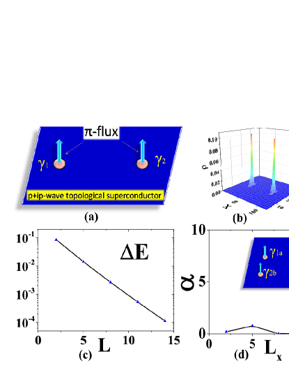
Figure 6: (color online) (a) Illustration of two Majorana bound states trapped by $\pi$-fluxes in $p_{x}+ip_{y}$ topological superconductor; (b) The particle density distribution of Majorana zero modes around two $\pi$-fluxes; (c) The energy splitting $\Delta E_{\mathrm{el}}$ via $L$ (the distance between the two Majorana bound states); (d) The gap-ratio.

In the first example, we studied the MFs around vortices in a 2D $p_{x}+ip_{y}$ topological SC. The Hamiltonian of a $p_{x}+ip_{y}$ SC on a square lattice is written asRead00

$$\hat{H}_{\mathrm{pip}} =-t\sum\limits_{j}\sum\limits_{\widehat{\mu}=\widehat{x},\widehat{y}}(c_{j+\widehat{\mu}}^{\dagger}c_{j}+c_{j-\widehat{\mu}}^{\dagger}c_{j})-\mu\sum\limits_{j}c_{j}^{\dagger}c_{j}$$

$$+\sum\limits_{j}[\Delta(c_{j+\widehat{x}}^{\dagger}c_{j}^{\dagger}+ic_{j+\widehat{y}}^{\dagger}c_{j}^{\dagger})+H.c.],$$ (11)

where $c_{j}$ is an electronic annihilation operator, $\mu$ is the chemical potential, $\Delta$ is the SC pairing-order parameter and $t$ is the hopping strength. The lattice constant was set to unity in this paper. In the following, we chose the parameters as $t=1,$ $\mu=-1,$ $\Delta=0.4$. The ground state was the weak-pairing phase that is a (strong) topological SC.

We first studied two MFs ($\gamma_{1}$, $\gamma_{2}$) around two vortices with numerical calculations on a $120\times 40$ lattice. We found that there exists a Majorana zero mode around each vortex. Note the particle density around two $\pi$-fluxes in Fig.6.(b). When there are two fluxes nearby, inter-flux quantum tunneling occurs and the two MFs couple. Fig.6.(c) shows the energy splitting $\Delta E_{\mathrm{el}}$. Next, we studied four coupled MFs of vortices, $\gamma_{1a}$, $\gamma_{1b}$, $\gamma_{2a}$, $\gamma_{2b},$ that formed an $L_{x}\times L_{y}$ square (a dimerized Majorana ring). See inset in Fig.6.(d). By fixing $L_{y}$ at $6$ and varying $L_{x}$, we calculated the gap ratio $\alpha$ and show the result in Fig.6.(d), in which one can see a very small gap ratio. There is no evidence of the first order TQPT. Therefore, we identified the MFs induced by the vortices in $p_{x}+ip_{y}$ topological SCs to be topological MFs. It is obvious that this conclusion (topological MFs in 2D $p_{x}+ip_{y}$ topological SCs) is consistent with earlier resultskou1 .

V.2 Majorana bound states in an $s$-wave topological superconductor with Rashba spin-orbital coupling

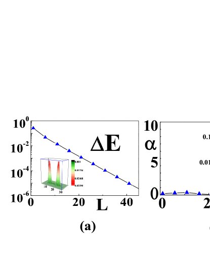
Figure 7: (color online) (a) The energy splitting $\Delta E_{\mathrm{el}}$ via the length $L$ of two vortices. The inset in (a) shows the particle density distribution of the Majorana bound states; (b) The gap-ratio of four Majorana bound states. The inset in (b) shows two positive energy levels of four coupled Majorana bound states.

The second model is MFs in an $s$-wave SC with Rashba spin-orbital (SO) coupling on a square latticeMS ; Lutchyn10 ; Oreg10 ; Sau10 . The Hamiltonian is given by $\hat{H}_{\mathrm{s-wave-SO}}=\hat{H}_{\mathrm{kin}}+\hat{H}_{\mathrm{so}}+\hat{H}_{\mathrm{sc}}$ where the kinetic energy term $\hat{H}_{\mathrm{kin}}$, the Rashba SO coupling term $\hat{H}_{\mathrm{so}}$, and the SC pairing term $\hat{H}_{\mathrm{sc}}$ are given as

$$\hat{H}_{\mathrm{kin}} =-t{\displaystyle\sum\limits_{j\sigma}}{\displaystyle\sum\limits_{\widehat{\mu}=\widehat{x},\widehat{y}}}(c_{j+\widehat{\mu}\sigma}^{\dagger}c_{j\sigma}+c_{j-\widehat{\mu}\sigma}^{\dagger}c_{j\sigma})$$ (12)

$$-\mu{\displaystyle\sum\limits_{j\sigma}}c_{j\sigma}^{\dagger}c_{j\sigma}-h{\displaystyle\sum\limits_{j}}(c_{j\uparrow}^{\dagger}c_{j\uparrow}-c_{j\downarrow}^{\dagger}c_{j\downarrow}),$$

$$\hat{H}_{\mathrm{so}} =-\lambda{\displaystyle\sum\limits_{j}}[(c_{j-\widehat{x}\downarrow}^{\dagger}c_{j\uparrow}-c_{j+\widehat{x}\downarrow}^{\dagger}c_{j\uparrow})$$

$$+i(c_{j-\widehat{y}\downarrow}^{\dagger}c_{j\uparrow}-c_{j+\widehat{y}\downarrow}^{\dagger}c_{j\uparrow})]+H.c.,$$

$$\hat{H}_{\mathrm{sc}} =-\Delta{\displaystyle\sum\limits_{j}}(c_{j\uparrow}^{\dagger}c_{j\downarrow}^{\dagger}+H.c.).$$

Here, $c_{j\sigma}$ ($c_{j\sigma}^{{\dagger}}$) annihilates (creates) a fermion at site $j=(j_{x},$ $j_{y})$ with spin $\sigma=(\uparrow,$ $\downarrow)$, $\widehat{\mu}=\widehat{x}$ or $\widehat{y}$, which is a basic vector for the square lattice. $\lambda$ serves as the SO coupling constant and $\Delta$ as the s-wave SC pairing-order parameter. $\mu$ is the chemical potential and $h$ is the strength of the Zeeman field. The lattice constant was set as unity. The parameters were chosen to be $t=1,$ $\mu=-4,$ $h=0.8,$ $\lambda=0.5,$ $\Delta=0.5.$ In this case, the ground state was a (strong) topological SC.

We then studied two MFs around two vortices through numerical calculations on a $100\times 24$ lattice. The particle distribution of the Majorana zero mode is given in the inset in Fig.7.(a). The results of the energy splitting $\Delta E_{\mathrm{el}}$ via the distance of the two vortices $L$ are given in Fig.7.(a). Next we studied four coupled MFs around the vortices $\gamma_{1a}$, $\gamma_{1b}$, $\gamma_{2a}$, and $\gamma_{2b}$, that formed an $L_{x}\times L_{y}$ square (a dimerized Majorana ring). We fixed $L_{y}$ to be $6$ and varied $L_{x}$. The gap ratio is shown in Fig.7.(b). One can see a small gap ratio. As a result, we conclude that MFs in an $s$-wave topological superconductor with Rashba SO coupling obey topological polygon sign rulekou2 .

V.3 Majorana bound states in a nanowire-SC hybridization system

The third model was a 1D semiconducting nanowire with strong spin-orbital coupling in a Zeeman field, proximity-coupled to an s-wave superconductor. See the illustration in Fig.8.(a). The Hamiltonian of the system is $\hat{H}_{\mathrm{nano-SC}}=\hat{H}_{\mathrm{1D}}+\hat{H}_{\mathrm{sc}}$, where $\hat{H}_{\mathrm{1D}}$ describes a 1D semiconducting nanowire; it is written as

$$\hat{H}_{\mathrm{1D}} =-t_{s}\sum\limits_{j\sigma}\sum\limits_{\widehat{\mu}=\widehat{x}}(c_{j+\widehat{\mu}\sigma}^{\dagger}c_{j\sigma}+c_{j-\widehat{\mu}\sigma}^{\dagger}c_{j\sigma})+H.c.$$ (13)

$$-\lambda\sum\limits_{j}(c_{j-\widehat{x}\downarrow}^{\dagger}c_{j\uparrow}-c_{j+\widehat{x}\downarrow}^{\dagger}c_{j\uparrow})-h\sum\limits_{j}(c_{j\uparrow}^{\dagger}c_{j\uparrow}-c_{j\downarrow}^{\dagger}c_{j\downarrow})$$

$$-\Delta\sum\limits_{j}c_{j\uparrow}^{\dagger}c_{j\downarrow}^{\dagger}-\mu\sum\limits_{j\sigma}c_{j\sigma}^{\dagger}c_{j\sigma},$$

$\hat{H}_{\mathrm{sc}}$ describes the 2D superconductor out of 1D semiconducting nanowire and is written as

$$\hat{H}_{\mathrm{sc}} =-t\sum\limits_{j\sigma}\sum\limits_{\widehat{\mu}=\widehat{x},\widehat{y}}(c_{j+\widehat{\mu}\sigma}^{\dagger}c_{j\sigma}+c_{j-\widehat{\mu}\sigma}^{\dagger}c_{j\sigma})$$

$$-\mu\sum\limits_{j\sigma}c_{j\sigma}^{\dagger}c_{j\sigma}-\Delta\sum\limits_{j}(c_{j\uparrow}^{\dagger}c_{j\downarrow}^{\dagger}+H.c.),$$ (14)

where $c_{j\sigma}$ is an electronic annihilation operator and $t$ $(t_{s}),$ $\mu,$ $\Delta,$ $\lambda,$ $h$ denote the hopping parameters, the chemical potential, the (induced) pairing order parameters, the spin-orbit coupling strength and the Zeeman field, respectively. The lattice constant was set to be unity. In the following, we chose the parameters as $t_{s}=1,$ $h=0.8,$ $\mu=-2,$ $\lambda=0.5,$ $\Delta=0.4,$ $t=0.4.$ The ground state of the system is a (weak) topological SC.

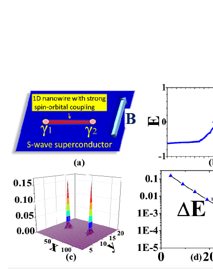
Figure 8: (color online) (a) Illustration of nanowire-SC hybridization system; (b) Two Majorana bound states with zero energy; (c) Particle distribution of Majorana bound states at the ends of the nanowire on s-wave SC; (d) The energy splitting of two Majorana bound states. The inset in (d) shows a very tiny $J_{2}$.

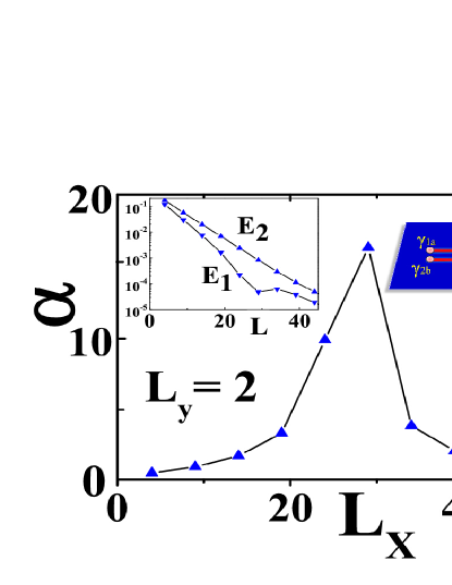
Figure 9: (color online) The gap-ratio of the four Majorana bound states in nanowire-SC hybridization system. The right inset illustrates two semiconducting nanowires on an SC system. The left inset shows two positive energy levels of four Majorana bound states.

Then, treating a nanowire by numerical calculations on a $120\times 20$ lattice, we found that there are two Majorana zero modes ($\gamma_{1}$, $\gamma_{2}$) at two ends of a nanowire. See the illustration in Fig.8.(a). There exist two zero modes in the energy gap shown in Fig.8.(b). In Fig.8.(c), we plot the particle distribution of the zero modes. The relationship between the energy splitting $\Delta E_{\mathrm{el}}$ and the length $L$ of the nanowire is shown in Fig.8.(d). Next, we considered two parallel 1D semiconducting nanowires on an SC. See the right inset in Fig.9. Here the low energy physics is dominated by four coupled MFs, $\gamma_{1a}$, $\gamma_{1b}$, $\gamma_{2a}$, $\gamma_{2b},$ that form an $L_{x}\times L_{y}$ square (or a dimerized Majorana ring). We fixed the distance between two parallel nanowires to be $L_{y}=2$ and then changed the length $L_{x}$ of the two nanowires. The left inset of Fig.9 shows the two positive energy levels from four MFs of the two nanowires vs. $L_{x}$. In Fig.9, the gap ratio $\alpha$ is obtained. From Fig.9, one can see that the maximum value of $\alpha$ reached $17$ at $L_{x}=30$. The sharp enhancement of the gap ratio $\alpha$ is obviously the consequence of a first order TQPT. As a result, we conclude that the MFs in the nanowire-SC hybridization system obey normal polygon sign rule.

V.4 Majorana bound states in a p-wave superconductor on a honeycomb lattice

The fourth model was MFs in a 2D p-wave superconductor on a honeycomb lattice. The Hamiltonian of a p-wave superconductor for spinless fermions on a honeycomb lattice is written askou

$$\hat{H}_{\mathrm{p-wave}}=-t\sum\limits_{\left\langle ij\right\rangle}c_{i}^{\dagger}c_{j}-t^{\prime}\sum\limits_{\left\langle\left\langle ij\right\rangle\right\rangle}c_{i}^{\dagger}c_{j}-\sum\limits_{\left\langle ij\right\rangle}\Delta_{ij}c_{i}^{{\dagger}}c_{j}^{\dagger}+H.c.,$$ (15)

where $t$ $(t^{\prime})$ denote the strengths of nearest (next nearest) neighbor hopping. The p-wave pairing order parameters are defined by $\Delta_{j,j+\mathbf{a}_{1}}=-\Delta_{j,j+\mathbf{a}_{2}}=\Delta$, $\Delta_{j,j+\mathbf{a}_{3}}=0$. $\mathbf{a}_{\alpha}$ $(\alpha=1,2,3)$ denotes a vector that connects the nearest neighbor sites $i$ and $i+\mathbf{a}_{\alpha}.$ Along the red links in Fig.10.(a) and Fig.10.(c), the SC order parameter is finite; along black links, the SC order parameter is zero. The lattice constant is set to be unity. We chose $t=1,$ $t^{\prime}=0.01,$ $\Delta=1.34$ in this section. Here the ground state is a (weak) topological SC.

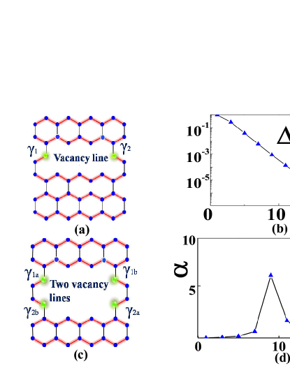
Figure 10: (color online) (a) Illustration of two Majorana bound states induced by a line defect; (b) The energy splitting $\Delta E_{\mathrm{el}}$ via the length $L$ of the line defect; (c) Illustration of four Majorana bound states induced by two line defects; (d) The gap-ratio of the four coupled Majorana bound states induced by two parallel line defects.

In Ref.kou , it was found that there exist two Majorana modes localized at the ends of the line defect (LD), $\gamma_{1}$, $\gamma_{2}$. See the illustration in Fig.10.(a). The end of an LD can be considered to be the boundary of a one-dimensional p-wave SCKitaev01 . Thus, each end of the LD traps a dangling Majorana zero mode. We studied two MFs around a LD with numerical calculations on a $100\times 50$ lattice and give the results of the energy splitting $\Delta E_{\mathrm{el}}$ via the length $L$ of the LD in Fig.10.(b). Then, as shown in Fig.10.(c), we studied four coupled MFs of two parallel LDs that formed an $L_{x}\times L_{y}$ square (a dimerized Majorana ring). The distance between the two parallel LDs was fixed to be $2$ (or $L_{y}=2$). We varied the length of the LDs, $L_{x}$. The results of the gap ratio $\alpha$ are given in Fig.10.(d), in which the maximum value of $\alpha$ reaches $6.5$ at $L_{x}=9$. These results indicate a first order TQPT with level-crossing. Thus, the MFs in p-wave superconductors on honeycomb lattice also obey normal polygon sign rule.

VI Discussion and conclusion

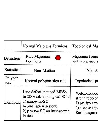
Figure 11: (color online) The difference between normal Majorana Fermions and topological Majorana Fermions.

In the end, we draw our conclusions (see the summary in Fig.11). We have pointed out that in 2D topological superconductors, there exist two classes of MFs: MFs obeying normal polygon sign rule and MFs obeying topological polygon sign rule. A numerical approach was proposed to identify the polygon sign rule of the MFs by looking for the signature of a first order TQPT of multi-MFs. Applying the approach to study several 2D topological systems, we found that vortex-induced MFs in 2D strong topological SCs (a $p_{x}+ip_{y}$ topological superconductor in Sec.VI.A and an s-wave topological superconductor with Rashba spin-orbital coupling in Sec.VI.B) obey topological polygon sign rule and line-defect-induced MFs in 2D weak topological SCs (nanowire-SC hybridization system in Sec.VI.C, p-wave superconductor on honeycomb lattice in Sec.VI.D) obey normal polygon sign rule.

* * *

This work is supported by National Basic Research Program of China (973 Program) under the grant No. 2011CB921803, 2012CB921704 and NSFC Grant No. 11174035, 11474025 and SRFDP.

References

- (1) E. Majorana, Soryushiron Kenkyu 63 149 (1981).
- (2) F. Wilczek, Nature Phys. 5 614 (2009).
- (3) M. Leijnse and K. Flensberg, arXiv:1206.1736.
- (4) A.Y. Kitaev, Phys. Usp. 44, 131 (2001).
- (5) L. Fu and C.L. Kane, Phys. Rev. Lett. 100, 096407 (2008).
- (6) R. M. Lutchyn, J.D. Sau, and S. Das Sarma, Phys. Rev. Lett. 105, 077001 (2010).
- (7) Y. Oreg, G. Refael, and F. von Oppen, Phys. Rev. Lett. 105, 177002 (2010).
- (8) J. D. Sau, R. M. Lutchyn, S. Tewari, and S. Das Sarma, Phys. Rev. Lett. 104, 040502 (2010).
- (9) J. Alicea, Phys. Rev. B 81, 125318 (2010).
- (10) A. C. Potter and P. A. Lee, Phys. Rev. Lett. 105, 227003 (2010).
- (11) J. Alicea, Y. Oreg, G. Refael, F. von Oppen, and M.P.A. Fisher, Nature Phys. 7, 412 (2011).
- (12) B. I. Halperin, Y. Oreg, A. Stern, G. Refael, J. Alicea, and F. von Oppen, Phys. Rev. B 85, 144501 (2012).
- (13) T. D. Stanescu and S. Tewari, J. Phys.: Condens. Matter 25, 233201 (2013).
- (14) V. Mourik, K. Zuo, S.M. Frolov, S.R. Plissard, E.P.A.M. Bakkers, and L.P. Kouwenhoven, Science 336, 1003 (2012).
- (15) A. Das, Y. Ronen, Y. Most, Y. Oreg, M. Heiblum, and H. Shtrikman, Nature Phys. 8, 887 (2012).
- (16) M. T. Deng, C. L. Yu, G. Y. Huang, M. Larsson, P. Caroff, and H. Q. Xu, Nano Lett. 12, 6414 (2012).
- (17) L. P. Rokhinson, X. Liu, and J. K. Furdyna, Nat. Phys. 8, 795 (2012).
- (18) H. O. H. Churchill, V. Fatemi, K. Grove-Rasmussen, M. T. Deng, P. Caroff, H. Q. Xu, and C. M. Marcus, Phys. Rev. B 87, 241401(R) (2013).
- (19) A. Kitaev, Ann. Phys. 321, 2 (2006).
- (20) C. Nayak, S. H. Simon, A. Stern, M. Freedman, and S. Das Sarm, Rev. Mod. Phys. 80, 1083 (2008).
- (21) M. H. Freedman, M. Larsen, Zhenghan Wang, Math. Phys. 227, 605 (2002).
- (22) S. Das Sarma, M. Freedman, and C. Nayak, Phys. Rev. Lett. 94, 166802 (2005).
- (23) L. S. Georgiev, Phys. Rev. B 74, 235112 (2006); L. S. Georgiev, Nucl. Phys. B 789, 552 (2008).
- (24) G. Moore and N. Read, Nucl. Phys. B 360, 362 (1991).
- (25) N. Read and D. Green, Phys. Rev. B 61, 10267 (2000).
- (26) D. A. Ivanov, Phys. Rev. Lett. 86, 268 (2001).
- (27) C. Nayak, S. H. Simon, A. Stern, M. Freedman, and S. Das Sarma, Rev. Mod. Phys. 80, 1083 (2008).
- (28) J. Alicea, Rep. Prog. Phys. 75, 076501 (2012).
- (29) Y. J. Wu, J. He, S. P. Kou, Phys. Rev. A. 90, 022324 (2014).
- (30) V. Lahtinen, A. W. Ludwig, J. K.Pachos, and S. Trebst, Phys. Rev. B 86, 075115 (2012).
- (31) J. Zhou, S. Z. Wang, Y. J. Wu, R. W. Li, and S. P. Kou, Physics Letters A 378, 2576 (2014).
- (32) J. Zhou, Y. J. Wu, R. L. Wu, S. P. Kou, EPL, 102 (2013) 47005.
- (33) E. Grosfeld and Ady Stern, Phys. Rev. B 73, 201303 (2006).
- (34) S. P. Kou and X.-G. Wen, Phys. Rev. B 82, 144501 (2010); 80, 224406 (2009).
- (35) M. Wimmer, et.al, Phys. Rev. Lett. 105, 046803 (2010).
- (36) T. L. Hughes, et.al, arXiv:1303.1539.
- (37) M. Sato, Y. Takahashi, and S. Fujimoto, Phys. Rev. Lett. 103, 020401 (2009).
- (38) E. Tang, J.-W. Mei, and X.-G. Wen, Phys. Rev. Lett. 106 236802 (2011).
- (39) K. Sun, Z. C. Gu, H. Katsura, and S. Das Sarma, Phys. Rev. Lett. 106, 236803 (2011).
- (40) T. Neupert, L. Santos, C. Chamon, and C. Murdy, Phys. Rev. Lett. 106, 236804 (2011).
- (41) Y. F. Wang, H. Yao, Z. C. Gu, C. D. Gong, D. N. Sheng, Phys. Rev. Lett. 108, 126805 (2012)