First detection of thermal radio jets in a sample of proto-brown dwarf candidates

Abstract

We observed with the Jansky Very Large Array at 3.6 and 1.3 cm a sample of 11 proto-brown dwarf candidates in Taurus in a search for thermal radio jets driven by the most embedded brown dwarfs. We detected for the first time four thermal radio jets in proto-brown dwarf candidates. We compiled data from UKIDSS, 2MASS, Spitzer, WISE and Herschel to build the spectral energy distribution (SED) of the objects in our sample, which are similar to typical Class I SEDs of young stellar objects. The four proto-brown dwarf candidates driving thermal radio jets also roughly follow the well-known trend of centimeter luminosity against bolometric luminosity determined for YSOs, assuming they belong to Taurus, although they present some excess of radio emission compared to the known relation for YSOs. Nonetheless, we are able to reproduce the flux densities of the radio jets modeling the centimeter emission of the thermal radio jets using the same type of models applied to YSOs, but with corresponding smaller stellar wind velocities and mass-loss rates, and exploring different possible geometries of the wind or outflow from the star. Moreover, we also find that the modeled mass outflow rates for the bolometric luminosities of our objects agree reasonably well with the trends found between the mass outflow rates and bolometric luminosities of YSOs, which indicates that, despite the “excess” centimeter emission, the intrinsic properties of proto-brown dwarfs are consistent with a continuation of those of very low mass stars to a lower mass range. Overall, our study favors the formation of brown dwarfs as a scaled-down version of low-mass stars.

1. Introduction

A crucial question that has been at the core of recent vigorous discussions is that of the formation of brown dwarfs. It is generally accepted that BDs form by gravitational instability of a very low-mass dense core, on a dynamical timescale and with initial elemental composition similar to low-mass stars, as opposed to planet formation, which could happen by aggregation of a rocky core from smaller planetesimals, on timescales longer than a dynamical time, and with elemental composition with an overall deficit on light elements (Whitworth et al., 2007). On the other hand, the underlying mechanism responsible for the formation of the very low-mass dense cores that would form BDs is not clear yet, and several scenarios were proposed to interpret the different observational results (see e. g., Reipurth & Clarke, 2001; Kroupa & Bouvier, 2003; Umbreit et al., 2005; Whitworth et al., 2007; André et al., 2012). After a major theoretical and observational effort during the last decade, statistical studies of low mass star forming regions essentially comparing the properties of low-mass young stars and BDs in the Class II/III stages (i. e., well after the main accretion phase, e. g., André et al. 1993) suggest that the dominant mechanism of BD formation is indistinguishable from that of low-mass stars (see e. g., Chabrier et al., 2014; Bayo et al., 2011, 2012; Scholz et al., 2012; Alves de Oliveira et al., 2013; Mužić et al., 2014). This is also favored by hydrodynamical simulations that routinely form BDs as a result of molecular cloud evolution, simultaneously reproducing the observed ratio of BDs to stars and the observed initial mass function (IMF) (e. g., Bate, 2012). Thus, it seems that the dominant formation mechanism of BDs cannot be easily distinguished from that of low-mass stars, and the most promising mechanism is the fragmentation of turbulent clouds, which naturally form very low-mass dense cores due to the effects of turbulence (see Luhman, 2012; Chabrier et al., 2014, for reviews). However, up to now the turbulent fragmentation scenario is not yet directly supported by observations of deeply embedded BDs, what we call here ‘proto-BDs’, i. e., BDs in the stage equivalent to the Class 0/I stage of low-mass YSOs (André et al., 1993), and the rest of the competing scenarios, mainly based on the halting of accretion of matter through ejection of protostellar embryos or disc fragments, and/or photo-erosion of pre-stellar cores, could still be possible (e. g., Stamatellos & Whitworth, 2009; Bate, 2012; Luhman, 2012). In fact, there are only two cases in the literature of Class 0/I proto-BDs (Lee et al., 2013; Palau et al., 2014), and further candidates are definitely needed in order to compare in a statistically significant base the properties of proto-BDs to the properties of low-mass YSOs. Since BDs are expected to form as a scaled-down version of low-mass stars in the the ‘turbulent fragmentation’ scenario, studying the properties of BDs in their most embedded phases of formation, and comparing their properties to the well-known relations established for low-mass protostars, should shed light on the formation mechanism of BDs.

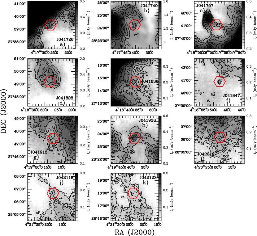
Figure 1.— Herschel SPIRE 250 $\mu$m continuum emission maps centered at the position of the proto-BD candidates in Taurus, indicated by red hexagons, that we observed with the JVLA. Contours are: a) 0.3, 0.33, 0.36, 0.39, 0.42, 0.45, 0.48, 0.51 mJy beam^-1; b) 1.20, 1.25, 1.30, 1.35, 1.40, 1.45, 1.50, 1.55, 1.60 mJy beam^-1; c) 0.30, 0.34, 0.37, 0.40, 0.44, 0.47, 0.50; d) 0.30, 0.33. 0.36 mJy beam^-1; e) 0.13, 0.16, 0.19, 0.22, 0.25, 0.28, 0.31, 0.34, 0.37, 0.40 mJy beam^-1; f) 0.13, 0.16, 0.19 mJy beam^-1; g) 0.19, 0.22, 0.27, 0.32, 0.37 mJy beam^-1; h) 0.30, 0.33, 0.36, 0.39, 0.42 mJy beam^-1; i) 0.06, 0.09, 0.12, 0.14, 0.17, 0.20, 0.23 mJy beam^-1; j) 0.06, 0.09, 0.12 mJy beam^-1; and k) 0.06, 0.09 mJy beam^-1, respectively.

The production of accretion-powered collimated ejections from the central protostellar object and disk is one of the processes characterizing the earliest phases of the evolution of high-, low-, and very-low mass YSOs (Lada, 1985; Shepherd & Churchwell, 1996; Li et al., 2014). These mass ejections can be usually traced in different ways: as narrow, highly-collimated jets of atomic and/or molecular gas, with $v\sim 100-1000$ km s^-1, observed from X-rays to mid-IR lines (Bally et al., 2007; Ray et al., 2007; Frank et al., 2014); or as less collimated but more massive molecular outflows with $v\sim 1-30$ km s^-1, typically observed using molecular gas tracers like CO, HCO⁺ or SiO at submillimeter/millimeter wavelengths. Another signpost of the ejection process is the presence of thermal radio jets, whose shock-ionized hydrogen atoms emit in the centimeter range with flat/positive spectral indices (e. g., Rodríguez, 1998; Beltrán et al., 2001; Reipurth et al., 2002). The centimeter emission of thermal radio jets in low-mass stars is thought to be free-free radiation produced by material (partially) ionized by the shock of the stellar wind with the surrounding gas (see e. g., Anglada, 1995; Curiel et al., 1987). Evidence for the connection between thermal radio jets and the wind from YSOs comes from the well-known trends between the centimeter luminosity and bolometric luminosity on one hand, and the centimeter luminosity and the momentum rate of the outflow on the other (e. g., Anglada, 1995; Bontemps et al., 1996; Shirley et al., 2007; AMI Consortium et al., 2011a; Phan-Bao et al., 2014b).

Several spectroastrometrically detected jets in BDs have been found in recent years (see e. g., Whelan et al., 2005, 2012; Joergens et al., 2012, 2013; Riaz et al., 2015), and a few molecular outflows have been detected, and imaged, in BDs or proto-BD candidates at submillimeter/millimeter wavelengths (Phan-Bao et al., 2008, 2014a; Palau et al., 2014; Monin et al., 2013). However, only very few Very Low Luminosity Objects and proto-BD candidates have been studied and detected in the centimeter range (André et al., 1999; Shirley et al., 2007; Palau et al., 2012), making it difficult to test whether or not proto-BDs follow the trend between centimeter luminosity and bolometric luminosity.

In this work, we present the results of the first search for thermal radio jets in a sample of proto-BD candidates. Sources were chosen from the sample of 12 proto-BD candidates selected by Barrado et al. (2009) and Palau et al. (2012) from Spitzer color–color and color–magnitude diagrams.

All these sources have red infrared colors and two of them (J041757 and J042118) were observed and detected at 350 $\mu$m with the Caltech Submillimeter Observatory (CSO) 10-m telescope, where we detected two (small) dust condensations associated with the Spitzer objects and condensations visible in Herschel maps at 160 and 250 $\mu$m, respectively. We derived a mass for the gas traced by the dust emission of 1–10 M${}_{\textrm{J}}$ and 0.3-3 M${}_{\textrm{J}}$ for J041757 and J042118, respectively. We also detected emission in J041757 at 3.6 and 6 cm in two VLA configurations, with a spectral index indicative of free-free thermal emission (Palau et al., 2012). Unfortunately, problems with the calibration in the VLA-B configuration prevented us from having a good flux calibration for the resolved emission. Nonetheless, the source was an excellent candidate to have emission from a thermal radio jet, which was only pending to be confirmed with new observations. Additionally, we found an excess in blue-shifted emission, possibly indicating the blue wing of an outflow, around the position of J041757 in the IRAM 30-m spectra of the ¹²CO (1–0) line. The SEDs that we could derive from the numerous multi-wavelength observations that our group had obtained (Barrado et al., 2009; Palau et al., 2012) allowed us to derive for our sources bolometric temperatures, $T_{\mathrm{bol}}$, of 150–280 K and 140  K, respectively, typical of Class I objects, and bolometric luminosities, $L_{\mathrm{bol}}$, $\lesssim 0.005$ and $<0.0023$ $L_{\sun}$, respectively, which would place them in the proto-BD regime. Palau et al. (2012) discussed the different possible types of objects that could be expected to explain the above observational data, but only the scenario of proto-BDs belonging to the Taurus Molecular Cloud consistently explains the properties of the emission ranging from optical, through IR to sub-mm wavelengths.

The structure of this paper is as follows: we describe the selected sample and the observations carried out with the JVLA in Section 2. Section 3 contains the results at 1.3 and 3.6 cm, the resulting spectral indices and the calculated SEDs of the objects of our sample. We discuss the nature of our objects in Section 4, where they lie in the centimeter luminosity vs. bolometric luminosity plot, how we can model their emission and how all the results affect the formation mechanisms of proto-BDs. Finally, Section 5 presents the conclusions of our work.

2. Observations

2.1. JVLA

We observed 11 proto-BD candidates in Taurus at 1.3 and 3.6-cm with the Jansky Very Large Array (JVLA) of the National Radio Astronomy Observatory (NRAO). We selected the 11 sources in our initial sample that were associated with extended large scale emission in 250 $\mu$m maps of Herschel, and thus could be associated with gas and dust emission of the Taurus cloud. In Figure 1, we overlay the position of each Spitzer source on the 250 $\mu$m maps of Herschel, showing that all the Spitzer sources fall in projection in regions of extended submillimeter emission, and several of them coincide with local emission enhancements at the position of the Spitzer source.

The 1.3-cm observations were carried out in 2013 June 10, while those at 3.6-cm were performed in 2013 June 15. The correlator was set-up to use 8 GHz bandwidth per polarization for dual polarization mode at 1.3-cm, and 2 GHz bandwidth at 3.6-cm. Both sets of observations used 27 antennas in the VLA-C configuration. We used J0336$+$3218 as gain calibrator and 3C147 as flux calibrator for both wavelengths. Each observing track was shared by all the sources in the sample. J041757, our best proto-BD candidate, was observed at the beginning and at the end of each track for a total on-source time of $\sim 8$ min at 1.3 cm and $\sim 9$ min at 3.6 cm. The rest of the targets were observed for approximately $\sim 5$ min on-source time at 1.3-cm and $\sim 4.5$ min at 3.6 cm. Pointing observations for the 1.3 cm data were done at the beginning and in the middle of the track, using the X band, on J0336$+$3218. The flux calibration observations on 3C147 at 1.3 cm were performed at the end of the track, using J0541$+$5312 as pointing source. The total observing time was 1h43min at 1.3 cm and 1h12min at 3.6 cm.

Calibration and data reduction were performed using the Common Astronomy Software Application (CASA) package (McMullin et al., 2007) from the raw visibility data downloaded from the VLA archive as CASA measurement sets and following NRAO guidelines for calibration and imaging. We produced images using the common $uv$-range at 1.3 and 3.6 cm to sample comparable spatial scales at both wavelengths, and additionally used different weightings (Briggs’s robust parameter ranging from 2, natural weighting to $-2$, uniform weighting), so that the final beams at 1.3 and 3.6 cm are comparable. The average rms values are $\sim 16~{}\mu$Jy beam^-1 for 1.3 cm and $\sim 30~{}\mu$Jy beam^-1 for 3.6 cm. The average synthesized beam at 1.3 cm is $\sim 1.8^{\prime\prime}\times 1.6^{\prime\prime}$. At 3.6 cm, the average beams are $\sim 2.2^{\prime\prime}\times 1.8^{\prime\prime}$ for uniform weighting and $\sim 3.1^{\prime\prime}\times 2.5^{\prime\prime}$ for natural weighting.

Table 1List of Herschel observations used in this study

OBSIDs
1342190616	1342202090	1342202254
1342202256	1342216549	1342216550
1342241898	1342241899	1342242047

2.2. Herschel Space Observatory

The Taurus molecular clouds were observed by the Herschel Space Observatory as part of the Gould Belt Survey (André et al., 2010). A first set of observations was obtained in parallel mode using the PACS (at 70 $\mu$m and 160 $\mu$m) and SPIRE (250 $\mu$m, 350 $\mu$m, and 500 $\mu$m) instruments simultaneously. The complete list of observations used in this study is reported in Table 1. More details about the observational strategy and depth of the maps can be found in André et al. (2010). The data were pre-processed using the Herschel Interactive Processing Environment (HIPE, Ott, 2010) version 12, and the calibration files version 65 for PACS and version 22.0 for SPIRE. The final maps were subsequently produced using Scanamorphos version 24.0 (Roussel, 2013), using its galactic option, as recommended to preserve large scale extended emission.

3. Results

3.1. 1.3- and 3.6-cm emission

We detected emission over 3$\sigma$ at both 1.3 and 3.6 cm in five sources of our sample (J041757, J041847, J041913, J041938, and J042123); only at 1.3 cm in J041836; and only at 3.6 cm in J041726 and J041740. For the rest of the candidates and/or bands, we only find upper limits.

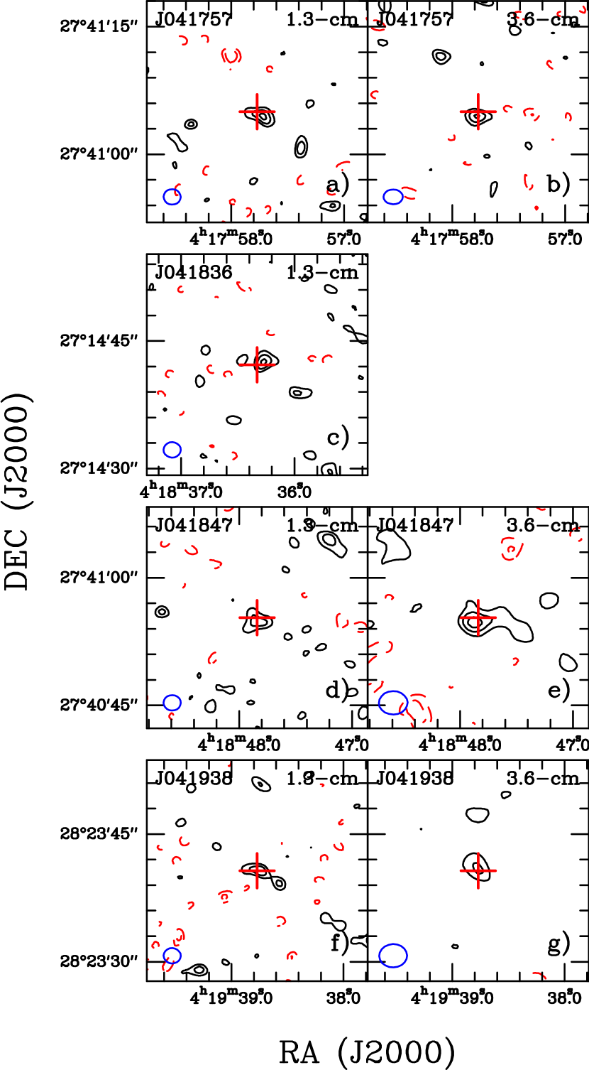
Figure 2.— JVLA maps of the 1.3- (left column) and 3.6-cm (right column) emission of the sources of our sample detected with partially resolved structures at 1.3 cm. Contours are -3,-2, 2, 3, …times the rms of the map, which from a) to g) are: 16, 31, 19, 20, 17, 20, and 25 $\mu$Jy beam^-1, respectively. The red crosses mark the position of the Spitzer sources presented in Barrado et al. (2009). The blue ellipse at the lower left corner of each panel indicates the beam size.

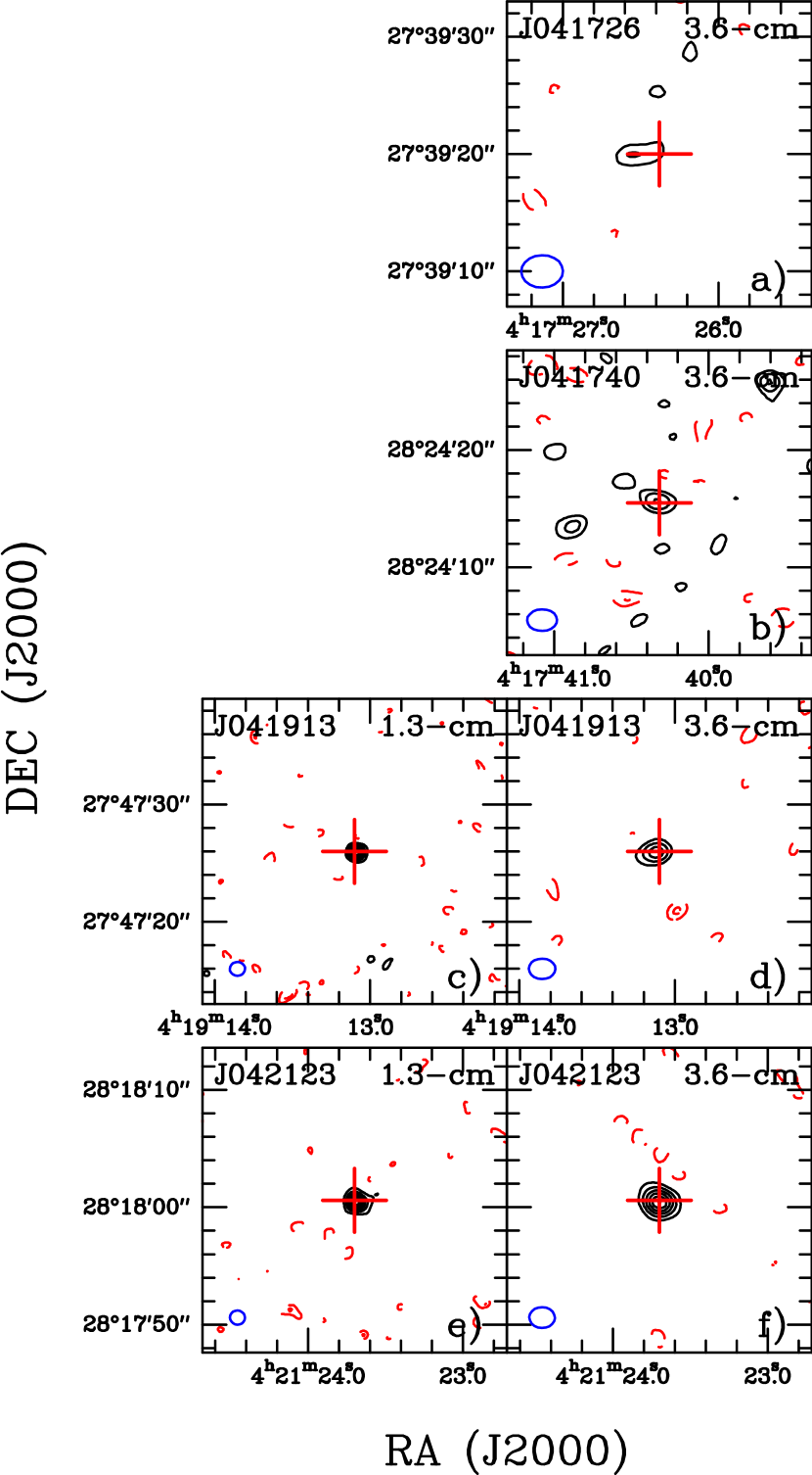
Figure 3.— JVLA maps of the 1.3- (left column) and 3.6-cm (right column) emission of the detected sources with point-like or undetected emission at 1.3 cm. Contours are: a) $-3$,$-2$, 2, 3, 4; b) $-3$,$-2$, 2, 3, 4; c) $-3$, $-2$, 3, 6, …; d) $-3$, $-2$, 3, 4, 5; e) $-3$, $-2$, 4, 9, …; f) $-3$, $-2$, 3, 6, …times the rms of the map, which from a) to f) are: 20, 25, 16, 50, 16, and 51 $\mu$Jy beam^-1, respectively. The red crosses mark the position of the Spitzer sources presented in Barrado et al. (2009). The blue ellipse at the lower left corner of each panel indicates the beam size.

Figure 2 presents the maps of the four sources in our sample that show slightly extended and faint ($\sim 0.1$ mJy beam^-1) emission at 1.3 cm: J041757, J041836, J041847, and J041938. For these sources, we fitted a 2D Gaussian function, and report the position and deconvolved sizes in Table 2. The typical deconvolved sizes are $\sim 3^{\prime\prime}\times 2^{\prime\prime}$, and the resulting positions of the sources match very well the position of the Spitzer sources, within the uncertainties. In addition, these four slightly extended 1.3 cm sources show weak and almost unresolved emission at 3.6 cm (except for J041836, not detected at 3.6 cm).

Figure 3 shows the maps of the sources with unresolved emission. J041740 is detected at 4$\sigma$ at 3.6 cm only, and is almost unresolved, while J041726 is just barely detected at 3.2$\sigma$ at 3.6 cm. The sources J041913 and J042123 are clearly detected at both 1.3 and 3.6 cm, with intensity peaks between 0.3 and 0.9 mJy beam^-1, and signal-to-noise ratios $\sim 8$–25. The emission from these last two unresolved sources is significantly more intense than the emission of the rest of the detected sources of our sample. The positions of these two sources also agree very well with the positions of the Spitzer sources.

Columns 9 and 10 of Table 2 list the peak intensities and flux densities calculated for all the detected sources (or the corresponding upper limits) measured inside the 1$\sigma$ contour. The flux densities for the sources with partially resolved emission are between 0.09 and 0.15 mJy, while the two bright unresolved sources have larger flux densities by factors of 2 to 8.

Column 11 of Table 2 shows the calculated spectral indices from the flux densities measured in the detected sources of our sample. We calculate the spectral index, $\alpha$ as (Kraus, 1986)

$$\alpha=\frac{\mathrm{ln}(S_{\nu_{1}}/S_{\nu_{2}})}{\mathrm{ln}(\nu_{1}/\nu_{2})}$$ (1)

where $S_{\nu}$ is the measured flux density at a given frequency $\nu$. For the sources with detection at only one frequency, we used an upper limit of 3$\sigma$ for the flux density. The resulting spectral indices show that the four sources with faint and partially resolved 1.3-cm emission have spectral indices compatible with being $>-0.1$. The uncertainties in the determination of the spectral indices are relatively large, given the low S/N of most of the detections, which will only be improved with new and more sensitive observations. At the same time, the ratios between the flux densities at 1.3 and 3.6 and, in the case of J041757, an independent measure of the spectral index confirming the result of Palau et al. (2012), indicate that it is unlikely that the spectral indices of these sources are significantly $<-0.1$. On the other hand, the spectral indices for the two point-like sources J041913 and J042123, and for J041740, are clearly negative, and remain $<-0.1$ even taking into account the associated uncertainties. J041726, which is barely detected at 3.6-cm, shows a positive upper limit for the spectral index, but in this case we only have an upper limit for the emission at 1.3 cm.

3.2. Spectral energy distribution of the sources

In Figure 4, we present the SEDs of the sources of our sample, built using UKIDSS, 2MASS (Skrutskie et al., 2006), and WISE databases, and measuring the fluxes in Spitzer (IRAC and MIPS), and Herschel (PACS and SPIRE) archive images (see Section 2.2). We additionally included the measurements at 350 $\mu$m reported in Palau et al. (2012), and the data presented in this work using the JVLA at 1.3 and 3.6 cm. All these data are listed in Appendix A. The Herschel fluxes were obtained via aperture photometry. The values used for the apertures, inner and outer annulus radii of the background ring are (in this order): 10^′′, 10^′′, 20^′′ for all PACS bands, 20^′′, 20^′′, and 25^′′ for SPIRE 250 and 350 $\mu$m, and 30^′′, 30^′′, 50^′′ for SPIRE 500 $\mu$m. The corresponding aperture correction factors were applied. When no detection is present in the Herschel maps (after visual inspection), upper limits were computed as the standard deviation of several aperture photometry measurements performed around the source coordinates. There are no detections in any Herschel band for J041726, J041836, J041913, and J042019.

Table 2Parameters of the sources observed with the JVLA

				Deconvolved a
Source	Wavelength	Position a		ang. size	P.A.	$T_{\mathrm{bol}}$ b	$L_{\mathrm{bol}}$ b	$I_{\nu}$	$S_{\nu}$ c	$\alpha$	Type of
	(cm)	$\alpha$ (J2000)	$\delta$ (J2000)	(arcsec)	(deg.)	(K)	($L_{\sun}$)	(mJy beam-1)	(mJy)		source
J041726	1.3					$>197$	$<0.0015$	$<0.036$ d	$<0.04$ e	$<0.16\pm$$0.74$ e	?
	3.6	4:17:26.50	27:39:20.0	point source				0.05$\pm$0.02	0.04$\pm$0.02
J041740	1.3					389	0.0032	$<0.040$ d	$<0.04$ e	$<-$0.94$\pm$0.69  e	?
	3.6	4:17:40.34	28:24:15.7	$2.86\times 0.07$	57.3			0.10$\pm$0.03	0.09$\pm$0.03
J041757	1.3	4:17:57.73	27:41:04.5	$3.25\times 0.98$	65.6	226	0.0036	0.07$\pm$0.02	0.13$\pm$0.03	$-$0.06$\pm$0.45	radio jet
	3.6	4:17:57.78	27:41:04.4	$2.03\times 0.73$	$-88.9$			0.13$\pm$0.03	0.14$\pm$0.04
J041828	1.3					249	0.0011	$<0.045$ d
	3.6							$<0.123$ d			?
J041836	1.3	4:18:36.28	27:14:42.6	$2.05\times 1.36$	$-68.1$	$>377$	$<0.0033$	0.08$\pm$0.02	0.13$\pm$0.03	$\phantom{;}>$0.02$\pm$0.47 f	radio jet
	3.6							$<0.105$ d	$<0.12$ f
J041847	1.3	4:18:47.84	27:40:54.9	$3.28\times 2.12$	63.8	126	0.0041	0.08$\pm$0.02	0.15$\pm$0.04	0.43$\pm$0.42	radio jet
	3.6	4:18:47.86	27:40:54.8	$3.79\times 1.38$	$-81.4$			0.08$\pm$0.02	0.10$\pm$0.03
J041913	1.3	4:19:13.09	27:47:25.9	point source		$>201$	$<0.0018$	0.28$\pm$0.02	0.28$\pm$0.02	$-$0.44$\pm$0.16	?
	3.6	4:19:13.13	27:47:25.9	point source				0.42$\pm$0.05	0.42$\pm$0.05
J041938	1.3	4:19:38.77	28:23:40.7	$4.01\times 0.58$	68.4	147	0.0062	0.08$\pm$0.02	0.11$\pm$0.03	0.09$\pm$0.50	radio jet
	3.6	4:19:38.78	28:23:41.0	$4.50\times 0.23$	36.9			0.08$\pm$0.03	0.10$\pm$0.03
J042019	1.3					$>487$	$<0.0018$	$<0.041$ d			?
	3.6							$<0.205$ d
J042118	1.3					166	0.0020	$<0.036$ d			?
	3.6							$<0.132$ d
J042123	1.3	4:21:23.69	28:18:00.4	point source		646	— g	0.53$\pm$0.02	0.53$\pm$0.02	$-$0.64$\pm$0.09	radiogalaxy
	3.6	4:21:23.70	28:18:00.4	point source				0.94$\pm$0.05	0.94$\pm$0.07

^aObtained from fitting a 2D Gaussian function to the emission.

^b$T_{\mathrm{bol}}$ is calculated from the SED following (Chen et al., 1995) and $L_{\mathrm{bol}}$ is calculated integrating the SED, and assuming a distance $D=140$ pc. For J041726, J041836, J04193 and J042019, which are not detected in any Herschel band, we estimated $T_{\mathrm{bol}}$ and $L_{\mathrm{bol}}$ using the upper limit of PACS at 70 $\mu$m, and considered the resulting $T_{\mathrm{bol}}$ as a lower limit and the resulting $L_{\mathrm{bol}}$ as an upper limit.

^cFlux densities were measured inside the 1$\sigma$ contour of the emission.

^dUpper limit calculated as 3$\sigma$, where $\sigma$ is rms of the map.

^eCalculated using an upper limit for the 1.3-cm flux density, S_ν, $S_{\mathrm{lim}}=3\sigma$, where $\sigma$ is the rms of the map (Beltrán et al., 2001).

^fCalculated using an upper limit for the 3.6-cm flux density, S_ν, $S_{\mathrm{lim}}=3\sigma A^{0.7}$, where $\sigma$ is the rms of the map, and $A$ is the source area in beam units estimated from the 1.3-cm observations (Beltrán et al., 2001).

^gGiven the classification of this object as a radiogalaxy, the $L_{\mathrm{bol}}$ calculated from the SED is meaningless.

Figure 4 shows that the SEDs are in general flat in the range 2–100 $\mu$m, or peaking around 100 $\mu$m in some cases, such as J041757, J041847, J041938 and J042118. Interestingly, out of the 4 sources with SEDs peaking around 100 $\mu$m, 3 have flat or positive spectral indices in the centimeter range. In order to estimate this in a more quantitative way, we calculated the bolometric temperatures, $T_{\mathrm{bol}}$ (see Table 2), following Chen et al. (1995), and find them to range from 126 K to 650 K for all the sample. Thus, most of the sources of our sample present SEDs comparable to Class I young stellar objects. Two of the sources where we detect thermal radio jets, J041847 and J041938, have the lowest values of $T_{\mathrm{bol}}$, with $T_{\mathrm{bol}}<150$ K, which also suggests that they are probably Class 0/I sources. J041757 is also probably a young Class I object given the derived $T_{\mathrm{bol}}=226$ K. We also calculated the bolometric luminosities, $L_{\mathrm{bol}}$ (see Table 2), and find values ranging from 0.001 to 0.006 $L_{\sun}$, well within the proto-BD regime (according, e. g., to the evolutionary models of Baraffe et al. 2002).

4. Discussion

4.1. Nature of the objects

We can divide the detected sources in two distinct classes according to the spectral index calculated from the 1.3- and 3.6-cm continuum emission. The sources that show intense and unresolved emission, or no emission at 1.3 cm, J041740, J041913 and J042123, have clearly negative spectral indices consistent with being originated by non-thermal synchrotron emission, $\alpha\sim-0.6$ (e. g., Bieging & Cohen, 1989; Girart et al., 2002; Dzib et al., 2013). This emission is seen in T Tauri stars and radiogalaxies. In order to account for an extragalactic origin for our sources, we searched the VLA archive and the NRAO VLA Sky Survey (NVSS) (Condon et al., 1998) to check if there were any counterparts at longer wavelengths. We only found detections at several epochs of 21-cm radio continuum emission for J042123, which show a central object with two radio lobes on opposite sides of it, clearly tracing a radiogalaxy. We also searched the NASA Extragalactic Database for possible counterparts for our sources and only found J042123 to have an extragalactic counterpart, given the typical positional uncertainties in WISE and GALEX ($<1^{\prime\prime}$) and the positional uncertainties of our sources (determined from Spitzer/IRAC and the VLA, $<1^{\prime\prime}$). Thus, we classify J042123 as a radiogalaxy and do not consider it a proto-BD candidate any more. The classification of J041740 and J041913 remains unsettled due to lack of information.

On the other hand, the spectral indices for the four sources detected at 1.3 cm, with partially resolved emission, are compatible with flat or positive spectral indices, $>-0.1$ (already reported by Palau et al. 2012 for the case of J041757). These spectral indices are expected for optically thin ($\alpha\approx-0.1$) to partially optically thick thermal free-free emission. The origin of the thermal free-free emission in low-mass young stellar objects is usually related to shocks generated in an outflow (e. g., Curiel et al., 1989; Beltrán et al., 2001; González & Cantó, 2002; Lynch et al., 2013), and this kind of sources are designated as ‘thermal radio jets’. The 1.3-cm emission from these four objects also shows a marginal degree of elongation, which supports the idea that the emission is originated in a jet emanating from the substellar object. Thermal radio jets from young stellar objects are more easily seen at the most embedded Class 0/I phases, and three of the four objects where we find thermal radio jets present $T_{\mathrm{bol}}$ in the range 130–230 K, consistent with Class I phase $T_{\mathrm{bol}}$ near the border with the Class 0 phase. Thus, the detection of partially elongated thermal emission from several objects in our sample makes these four objects excellent candidates to Class I proto-BDs.

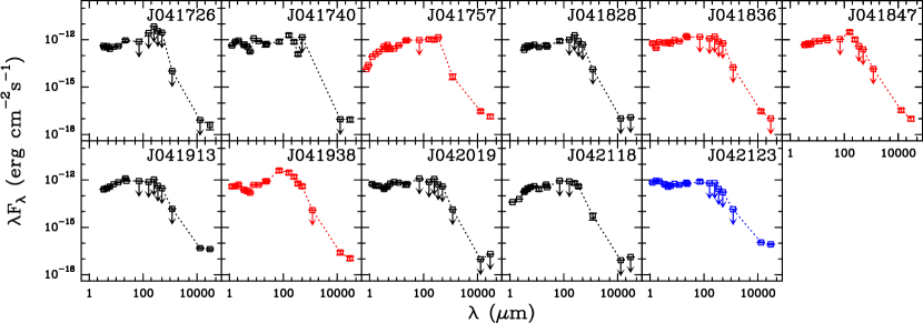
Figure 4.— SEDs for the 11 proto-BD candidates studied in this work. For most objects, Herschel PACS detects a source. The objects with SEDs in red are those for which a thermal radio jet has been detected. The object with the SED in blue corresponds to an identified radiogalaxy, through 21-cm continuum NVSS archival data (see Section 4.1).

4.2. Centimeter vs. bolometric luminosity

Figure 5 shows the centimeter luminosity at 3.6 cm measured in our JVLA observations versus the bolometric luminosity calculated from the SEDs of the objects of our sample associated with thermal radio jets and assuming that they belong to Taurus. We compare the results for our sample with the same variables measured for a sample of YSOs from Anglada (1995) and Shirley et al. (2007), where we also include the values for known VeLLOs with detected 3.6 cm emission (André et al., 1999; Shirley et al., 2007).

In general terms, the results for our sample of proto-BD candidates follow the trend expected for YSOs, extending to $L_{\mathrm{bol}}$ about one order of magnitude smaller. The relationship between the centimeter continuum luminosity and the bolometric luminosity of low-mass protostellar objects is interpreted to arise from the intrinsic relation between the stellar wind properties and the stellar mass. Since the stellar wind shocks against the surrounding high density material, ionizing the gas, more luminous young stellar objects are expected to have higher centimeter luminosity, due to stronger stellar winds and probably denser surrounding gas (see e. g., Curiel et al., 1987, 1989). However, the centimeter luminosities of the thermal radio jets of our sample (red crosses) present a systematic excess of about an order of magnitude from the relation found for YSOs (dashed line in Figure 5). This excess seems to be significant because the plotted bolometric luminosity is an upper limit to the true luminosity of the object (better approximated by the internal luminosity, Di Francesco et al. 2007).

However, we must be careful with our interpretation. The detected 3.6-cm luminosities of the thermal radio jets in our sample are very close to the detection limit we estimate from the rms of the undetected sources in our sample. With our data, we cannot discard the possibility that we are only seeing the upper tip of the more brilliant radio jets of a population of proto-BDs, while we cannot detect the emission of weaker radio jets that would lie closer to the fit of Shirley et al. (2007).

In order to account for this ‘extra’ centimeter emission, we discarded several mechanisms discussed in the literature, such as supersonic accretion onto a protostellar disk (Neufeld & Hollenbach, 1996; Shirley et al., 2007), because they do not seem feasible at all for the masses and accretion rates of the BD regime. Similarly, it seems very unlikely that the four detected radio jets in our sample have a burst, at the same time, of a variable (non-thermal) component with respect to the quiescent (thermal) component as found in the VeLLOs L1014-IRS (Shirley et al., 2007) and IRAM04191 (Choi, Lee, & Kang, 2014).

One possibility left is that the thermal radio jet or wind emanating from a proto-BD impacts against a medium with a higher density as compared to the case of low-mass star formation. This could be expected, as proto-BDs should not be highly efficient in creating cavities through the passage of their outflows. In Section 4.3, we use the same type of models used to reproduce the emission of thermal radio jets originating from low-mass YSOs and adapt them to the physical parameters of the BD regime, in order to explain the flux densities we detected for our thermal radio jets.

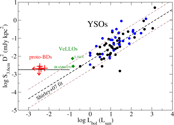
Figure 5.— Centimeter luminosity at 3.6 cm vs bolometric luminosity. Blue and black dots correspond to the data compiled by Anglada (1995) and Furuya et al. (2003), respectively, showing the relation for YSOs. Red plus signs correspond to the proto-BD candidates driving radio jets presented in this work. VeLLOs with detected 3.6 cm emission (André et al., 1999; Shirley et al., 2007) are shown as green squares. The horizontal black line indicates the typical detection limit from our 3.6-cm observations, calculated as the 3$\sigma$ value of the typical rms of our 3.6-cm maps, $\sim 30~{}\mu$Jy beam^-1. The black dashed-line is the fit performed by Shirley et al. (2007) to the YSOs. The two brown dashed lines indicate the standard deviation of the fit obtained by Shirley et al. (2007), calculated as $(\sum\limits_{i}(L_{\mathrm{cm}}^{i}(obs)-L_{\mathrm{cm}}^{i}(fit))^{2}/N)^{1/2}$.

4.3. Models of emission

Here we explore theoretical models which have been used to explain the emission of thermal radio jets from low-mass YSOs. We use the models developed by Curiel et al. (1987), González & Cantó (2002) and Rodríguez et al. (2012) in order to explain the observed radio-continuum emission (with thermal origin) from the sources of our sample. Curiel et al. (1987) calculated for the first time the radio-continuum emission (of thermal origin) produced by a plane-parallel shock wave. González & Cantó (2002) and Rodríguez et al. (2012) modeled the observed radio emission in low-mass stars as internal shocks, which are produced by intrinsic variability in the injection velocity, in a spherical wind and a bipolar outflow (with conical symmetry), respectively. We follow the approach of these authors to explore three possible geometries for the thermal emission detected in our sample of proto-BD candidates, since our observations are not able to fully resolve the geometry of the emitting region or to measure the degree of collimation of the thermal radio jets. We first calculate the emission produced by a plane-parallel shock wave in Section 4.3.1. We then apply the case of a stationary stellar wind with spherical symmetry in Section 4.3.2. Given that the partially resolved 1.3-cm emission maps show marginal elongations along a preferred direction, we also present in Section 4.3.3 the results of a variable conical wind model, collimated in a similar way as the YSOs winds. The assumed distance for all the models is $D=140$ pc, the adopted distance to the Taurus cloud (Loinard et al., 2005).

4.3.1 Plane-parallel shock wave

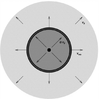
Figure 6.— Top: Schematic diagram showing a stellar wind with velocity $V_{0}$ which suddenly changes its value to $a\,V_{0}$ ($a>1$). The interaction between these outflows produces an internal working surface that propagates outwards with an intermediate speed $V_{WS}$. Figure taken from González & Cantó (2002). Bottom: Predicted flux densities at $\lambda=$1.3 cm (dashed line) and $\lambda=$3.6 cm (solid line) from a spherical wind with an internal single working surface. We have adopted an initial ejection velocity $V_{0}=50$ km s^-1, which suffers a sudden increase to $a\,V_{0}=200$ km s^-1. The mass-loss rate $\dot{m}=1.0\times 10^{-8}$ $M_{\sun}$ yr^-1 remains constant.

Curiel et al. (1987) developed an analytic model in order to calculate the free-free emission at radio frequencies produced in plane-parallel shock waves. These authors assumed that radiation is produced in the recombination zone, which is considered to be isothermal (T$\simeq$ 10⁴ K). The flux density is calculated using a correlation between the radio intensity and H_β intensity from the recombination zone. From an application of the model to an astrophysical source with a circular geometry, the flux density at radio frequencies in the optically thin regime ($\tau_{\nu}\ll$ 1, being $\tau$ the optical depth and $\nu$ the frequency) is given (in mJy) by,

$$S_{\nu}=1.84\times 10^{-4}\,\biggl{(}\frac{n}{10\,\mbox{cm}^{-3}}\biggr{)}\biggl{(}\frac{V}{100\,\mbox{km s}^{-1}}\biggr{)}$$ (2)

$$\times\,\biggl{(}\frac{\theta}{\mbox{arc sec}}\biggr{)}^{2}\biggl{(}\frac{\nu}{10\,\mbox{GHz}}\biggr{)}^{-0.1}$$

where $n$ is the pre-shock density, $V$ is the shock velocity, and $\theta$ is the angular diameter of the source. For shock velocities $V\sim 100$ km s^-1, the number of ionizing photons per atom produced by the shock wave is $\phi\sim 1$ (see, for instance, Kang & Shapiro, 1992). When we applied the model of Curiel et al. (1987) to our proto-BD candidates, we chose a source with an angular diameter $\theta=2^{\prime\prime}$ (Table 2). The adopted wind parameters The pre-shock density is calculated from the continuity equation, given the position of the shock wave with respect to the central source. Substitution of these values into Equation 2 gives the flux density $S_{\nu}=$ 0.1 mJy at a frequency $\nu=$ 8.33 GHz.

4.3.2 Stationary stellar wind with spherical symmetry

Let us now consider a spherical stationary stellar wind characterized by an ejection velocity $V_{0}$ and mass-loss rate $\dot{m}$. At $t=0$, the wind velocity suddenly increases to the value $a\,V_{0}$ (with $a>1$), while the mass-loss rate remains constant. This kind of variability was previously studied by González & Cantó (2002, 2008). Such variation in the wind parameters instantaneously produces (at the base of the wind) a two-shock wave structure (called a working surface) that propagates outwards over time with a speed $V_{WS}=a^{1/2}\,V_{0}$. Note that this value is intermediate between the slow and faster wind velocities (see top panel of Figure 6).

If we assume that the working surface is thin enough to be described by a unique distance $r_{WS}=r_{WS}(t)$, it is possible to determine the total optical depth $\tau_{WS}=\tau_{IS}+\tau_{ES}$ of the shocked layer, where $\tau_{IS}$ and $\tau_{ES}$ are the optical depths of the internal and external shocks, respectively, that bound the working surface. Then, we estimate the intensity emerging from each direction and calculate the flux density by integrating the intensity over the solid angle. That is,

$$S_{\nu}=2\pi B_{\nu}{\biggl{(}\frac{r_{WS}}{D}\biggr{)}}^{2}\int_{0}^{1}\biggl{(}1-e^{-2\tau_{\nu}(\mu)}\biggr{)}\mu d\mu$$ (3)

where $B_{\nu}(=2kT_{e}\nu^{2}/c^{2}$) is the Planck function in the Rayleigh-Jeans approximation, and $\mu$ = cos $\theta$, being $\theta$ the angle formed by each line of sight and the normal to the working surface.

The bottom panel of Figure 6 shows the results for a model for the radio continuum emission from a single working surface. The density fluxes were computed at frequencies $\nu=$8.33 GHz ($\lambda=$ 3.6 cm) and $\nu=$ 23.08 GHz ($\lambda$ = 1.3 cm). We chose representative parameters for BD sources: i) a stellar wind with an initial ejection velocity, $V_{0}=50$ km s^-1, that suddenly increases to 200 km s^-1 ($a=4$); and ii) a constant mass-loss rate $\dot{m}=1.0\times 10^{-8}$ M_⊙ yr^-1, an order of magnitude higher than the values derived from the measurements of Lee et al. (2013) and Palau et al. (2014) for two proto-BD candidates. Using these values, we obtain a working surface velocity $V_{WS}=$ 100 km s^-1, and consequently, shock velocities of $V_{is}=$ 100 km s^-1 and $V_{es}=$ 50 km s^-1 for the internal shock and the external shock, respectively. At the beginning, the working surface is optically thick at both wavelengths, and the flux grows as $t^{2}$ (since $r_{WS}\propto t$). When the shocked layer becomes optically thin (the transition time depends on the frequency as $\nu^{-1.05}$), the flux densities tend to constant values $S_{\mathrm{1.3~{}cm}}\simeq 0.075$ mJy and $S_{\mathrm{3.6~{}cm}}\simeq 0.083$ mJy, while the spectral index $\alpha_{1.3-3.6}\simeq$ tends to $-0.1$.

4.3.3 Variable conical outflow

We also computed the free-free emission from a bipolar outflow with conical symmetry. We assumed that the opening angle of the cones is $\theta_{a}$, and the inclination angle between the jet axis and the plane of the sky is $\theta_{i}$. We show a schematic diagram of the geometrical model in the top panel of Figure 7.

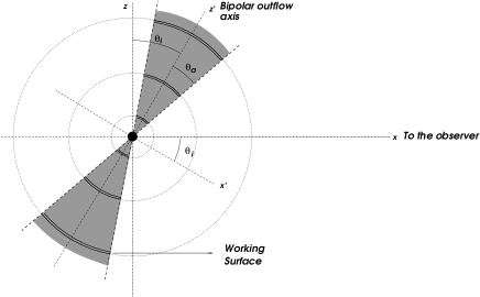
Figure 7.— Top: Schematic diagram showing a bipolar outflow with conical symmetry. The angles $\theta_{a}$ and $\theta_{i}$ are the opening angle of the cones and the inclination angle with the plane of the sky, respectively. Figure taken from Rodríguez et al. (2012). Bottom: Predicted flux densities at $\lambda=$ 1.3 cm (dashed line) and $\lambda=$ 3.6 cm (solid line) for a bipolar outflow with a sinusoidal ejection velocity. We assumed the following wind parameters: mean velocity $V_{w}=125$ km s^-1, amplitude $V_{c}=75$ km s^-1, oscillation frequency $\omega$= 6.28 yr^-1 (period $P=2\pi/\omega$= 1 yr), and constant mass-loss rate $\dot{m}=5\times 10^{-8}$ M_⊙ yr^-1. The opening angle of the cones is $\theta_{a}=$ 45^∘ with an inclination angle $\theta_{i}$= 45^∘.

For this model, we assumed a periodic variation in the injection velocity $V_{jet}$ and constant mass-loss rate $\dot{m}_{jet}$. In this scenario, the radiation is produced by internal working surfaces which move outwards over time from a central source. In particular, we consider a stellar conical outflow expelled with a sinusoidal variation in the injection velocity, $V_{jet}=V_{w}-V_{c}\,\mbox{sin}(\omega\tau)$, where $V_{w}$ is the mean velocity of the outflow, $V_{c}$ is the amplitude of the velocity variation, $w$ is the frequency, and $\tau$ is the injection time.

In order to obtain the flux density from the bipolar outflow, González (2002) and Rodríguez et al. (2012) found the conditions that indicate whether or not a working surface is intersected by a given line of sight. For this goal, this model described the internal working surfaces as polar caps (portions of spheres) whose physical sizes depend on the opening angle $\theta_{a}$ and their position from the central source. First, the total optical depth along each line of sight is estimated adding the optical depths of the working surfaces intersected by each line of sight. Then, the intensity emerging from each direction is calculated, and finally, the total flux emitted by the system is computed by integrating this intensity over the solid angle.

We present the predictions of our model in the bottom panel of Figure 7. We show a numerical example for the radio-continuum flux at $\lambda=1.3$ cm and $\lambda=3.6$ cm. The opening angle of the cones is $\theta_{a}=$ 45^∘ and the inclination angle is $\theta_{i}$= 45^∘. We assumed a mean velocity $V_{w}=125$ km s^-1, an amplitude $V_{c}=75$ km s^-1, and oscillation frequency $\omega$= 6.28 yr^-1 (that is, a period $P=2\pi/\omega$= 1 yr) and a constant mass-loss rate $\dot{m}=5\times 10^{-8}$ $M_{\sun}$ yr^-1. At a time $t\simeq$ 0.6 yr, the first working surfaces in both cones are formed. Initially, the flux densities increase, reaching maximum values of $S_{\mathrm{1.3~{}cm}}\simeq 0.078$ mJy and $S_{\mathrm{3.6~{}cm}}\simeq 0.085$ mJy at a time $t\simeq$ 0.85 yr. At this time, the model predicts a spectral index $\alpha_{1.3-3.6}\simeq$ $-0.084$, as expected from optically thin emission. Afterward, the flux at both frequencies decreases until new working surfaces are formed. The predicted fluxes show a periodic behavior with the same oscillation period ($P$ = 1 yr) of the injected velocity.

Table 3Predicted radio-continuum emission from proto-BD candidates

Model	Geometry	$V$ a	$\dot{m}$ b	$\nu$	Sν c
		(km s-1)	(M⊙ yr-1)	(GHz)	(mJy)
C87 d	plane-parallel	100 e	2.0 $\times$ 10-9	8.33	0.1
GC02 f	spherical	50–100 g	1.0 $\times$ 10-8	8.33	0.083
R12 h	conical	125 i	5.0 $\times$ 10-8	8.33	0.085

^aShock velocities.

^bMass wind/outflow rate.

^cOptically thin regime.

^dCuriel et al. (1987)

^eShock velocity (see Section 4.3.1).

^fGonzález & Cantó (2002)

^gExternal and internal shock velocities, respectively (see Section 4.3.2).

^hRodríguez et al. (2012)

ⁱMean velocity (see Section 4.3.3).

4.4. Proto-BDs as a scaled-down version of low-mass stars

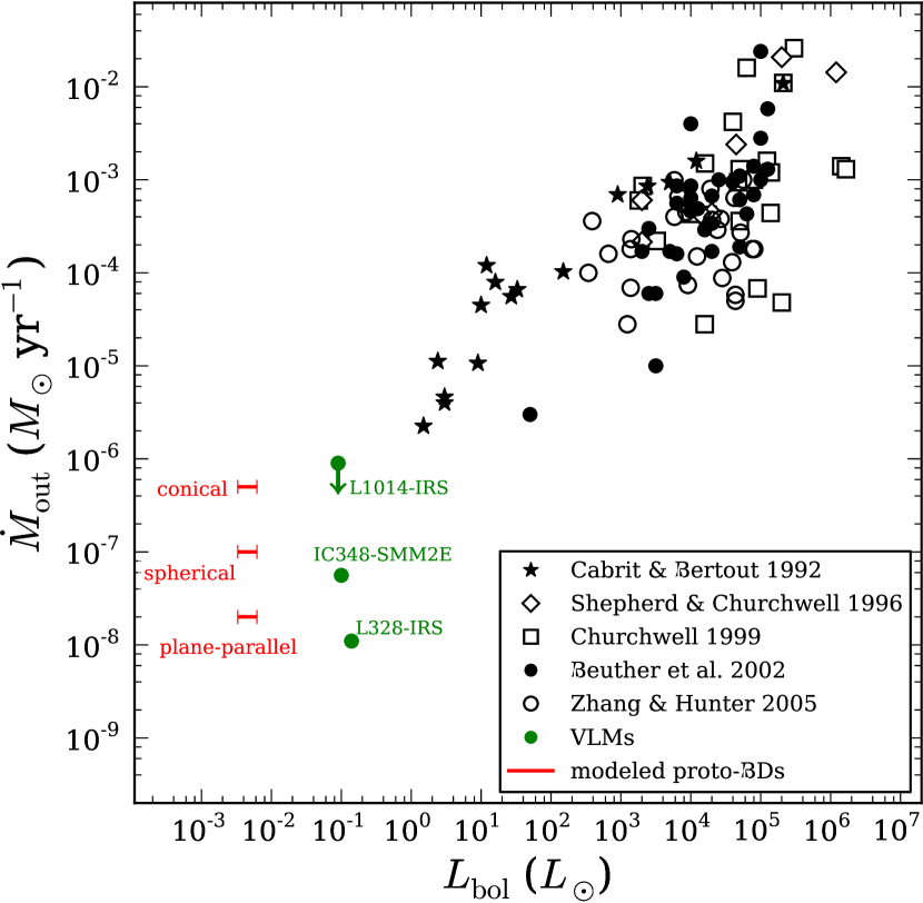
Figure 8.— Mass outflow rate, $\dot{M}_{\mathrm{out}}$, vs. bolometric luminosity, $L_{\mathrm{bol}}$, for a sample of YSOs taken from: Cabrit & Bertout (1992) (filled stars), Shepherd & Churchwell (1996) (open diamonds), Churchwell (1999) (open squares), Beuther et al. (2002) (filled circles), and Zhang et al. (2005) (open circles). The green dots indicate the values for three very low mass (VLMs) objects: a VeLLO, L1014-IRS Shirley et al. (2007), and two very young proto-BDs, IC348-SMM2E and L328-IRS (Lee et al., 2013; Palau et al., 2014). The horizontal red bars indicate the values for the $L_{\mathrm{bol}}$ of the proto-BD candidates powering the detected thermal radio jets and the three different modeled values of $\dot{M}_{\mathrm{out}}$ (see Section 4.3).

The models discussed in Section 4.3 allowed us to explore different possible geometries for the thermal emission detected in our sample of proto-BD candidates. In Table 3, we summarize the parameters used in the models to reproduce the observed centimeter emission, which range, for the mass loss rate, $\dot{m}$, from $2\times 10^{-9}$ to $5\times 10^{-8}$ $M_{\sun}$ yr^-1. Furthermore, we estimate a mass outflow rate, $\dot{M}_{\mathrm{out}}$, of the outflow that would be powered by this wind/conical outflow of about an order of magnitude higher, following e. g., estimates from Beuther et al. (2002) and our own estimates from the outflow parameters obtained for the deeply embedded Class 0/I proto-BD candidates IC348-SMM2E and L328-IRS (Lee et al., 2013; Palau et al., 2014). We show in Figure 8 how the mass outflow rates derived from the models lie in a typical relation found for young stellar objects for the mass outflow rate vs. the bolometric luminosity. We selected from the literature values corresponding to YSOs for a large range of $L_{\mathrm{bol}}$ and mass outflow rates. We used the values originally published by Cabrit & Bertout (1992), Shepherd & Churchwell (1996), Churchwell (1999), Beuther et al. (2002), and Zhang et al. (2005), and added the values of three very low mass objects (in green): the VeLLO L1014-IRS, and the proto-BDs IC348-SMM2E and L328-IRS. Figure 8 shows that the values inferred from our models are in agreement with the values expected if the trends found for young stellar objects are extrapolated to the luminosities of our proto-BD candidates. In fact, the conical model seems to achieve the best agreement with the extrapolation, and reproduces the observed radio continuum fluxes only needing a relatively large mass outflow rate compared to the ones calculated for the two proto-BD candidates IC348-SMM2E and L328-IRS. Nonetheless, this difference in mass outflow rate is of about the same order of magnitude as the typical variation found for $\dot{M}_{\mathrm{out}}$ along the whole range of $L_{\mathrm{bol}}$, which can easily be of 1–2 orders of magnitude. However, since a spherically symmetric wind can also explain the radio observations with lower mass outflow rates, we believe that further research is needed to establish which mechanism is operating or even if a combination of mechanisms is needed.

Thus, the models we used to explain the centimeter “excess emission” found in the $L_{\mathrm{cm}}$ vs. $L_{\mathrm{bol}}$ plot (Figure 5) require a range of mass outflow rates consistent with the values we would expect to find at very low bolometric luminosities if we would follow the trends found for YSOs. The models used in Section 4.3 are the same ones that are usually applied to low-mass YSOs, but with physical parameters adapted to the BD regime: smaller stellar wind velocities and smaller mass-loss rates than in low-mass YSOs. This supports the idea that the properties of proto-BDs are a continuation of the intrinsic properties of low-mass YSOs into the BD regime. There is also some evidence, although still confined to a few star forming clouds and relatively small number of objects, that the presence of thermal radio jets may be more common in the Class 0 phase of star formation, compared to Class I (see AMI Consortium et al., 2011a, b, 2012). As we mentioned in Section 3.2, three of the four objects where we detect thermal radio jets are probably Class 0/I or young Class I sources, given their relatively low $T_{\mathrm{bol}}$ values. These three sources are also among the four sources with the lower $T_{\mathrm{bol}}$ in the sample, which is what we would expect to find if the detection ratio in Class 0 and Class I YSOs is also extrapolated to the BD regime.

In order to explain the excess of centimeter emission with respect to the emission from YSOs, we propose that the initial pre-shock density could be be higher than what we assumed in our models, because proto-BDs could be less efficient in creating outflow cavities as compared to YSOs. This would also increase the efficiency of the shock and yield larger radio continuum fluxes. Additionally, the predictions of the models about the spectral indices of the centimeter emission are very consistent with our measurements, which are basically flat, indicating optically thin thermal emission. All these results, plus the first detection of thermal radio jets in proto-BD candidates, supports the idea that the formation mechanism of BDs is a scaled-down version of that of low-mass stars (Chabrier et al., 2014).

5. Conclusions

We observed with the JVLA at 3.6 and 1.3 cm a sample of 11 proto-BD candidates in Taurus, selected from Spitzer data, that were associated with extended emission in 250 $\mu$m maps of Herschel. We detected emission over 3$\sigma$ at both 1.3 and 3.6 cm in 5 sources (J041757, J041847, J041913, J041938, and J042123), only at 1.3 cm in J041836, and only at 3.6 cm in J041726 and J041740. Two of the sources, J041913 and J042123, are unresolved and clearly detected at both 3.6 and 1.3 cm, with intensity peaks between 0.3 and 0.9 mJy beam^-1, and show negative spectral indices, $\sim-0.6$, tracing non-thermal synchrotron emission. We found using 21-cm continuum archival data that J042123 is a radiogalaxy and discarded it from further consideration. We also constructed the SEDs for the remaining ten objects of our sample using data from near-IR to cm wavelengths and calculated their bolometric luminosities, $L_{\mathrm{bol}}$, and temperatures, $T_{\mathrm{bol}}$. We find that the bolometric temperatures of all the sources fall in the typical range of Class I protostellar objects. Globally, we detect a large fraction, 70%, of our proto-BD candidates at either 1.3 or 3.6 cm, which showcases the high sensitivity of the JVLA for this kind of studies.

Four of the 1.3-cm detected sources (J041757, J041836, J041847, and J041938) show partially extended, typically $\sim 3^{\prime\prime}\times 2^{\prime\prime}$, and faint emission $\sim 0.1$ mJy beam^-1, and their positions agree very well with the positions of the Spitzer sources. The emission of these four sources shows flat or slightly positive spectral indices, consistent with optically thin or partially thick thermal free-free emission associated with a thermal radio jet emanating from the protostar, which makes them excellent candidates to Class I proto-BDs. This would be the first detection of thermal radio jets in a sample of proto-BD candidates.

We also find that the four thermal radio jets show a centimeter emission excess when compared to the 3.6-cm vs. bolometric luminosity relationship found in low-mass YSOs. This excess is significant because $L_{\mathrm{bol}}$ is an upper limit to the true luminosity of the object and it is also difficult to explain invoking variable non-thermal emission or supersonic accretion onto a protostellar disk. We used models of the centimeter radio emission typically used for low-mass YSOs to explain this excess emission, assuming different geometries: a plane-parallel shock wave, a constant spherical stellar wind and a variable conical outflow; and adapting values for the mass loss rate and wind velocity to BDs, $\dot{m}\sim 2\times 10^{-9}$–$5\times 10^{-8}$$M_{\sun}$ yr^-1and $v\sim 50$–$100$ km s^-1. The models are able to reproduce approximately the measured fluxes at 3.6 cm. We also find that the modeled mass outflow rates for the bolometric luminosities of our objects agree reasonably well with the trends found between $\dot{M}_{\mathrm{out}}$ and $L_{\mathrm{bol}}$ for YSOs. This indicates that the same mechanisms are at work for YSOs and proto-BDs and supports the idea that the intrinsic properties of proto-BDs are a continuation to smaller masses of the properties of low-mass YSOs. We propose that if BDs are less efficient in creating outflow cavities than YSOs, the initial pre-shock density could be higher and there would be an increase of the radio continuum flux, which would more easily explain the “excess” centimeter luminosities.

These results, in addition to the detection of thermal radio jets and the SEDs of our candidates consistent with Class I sources, suggests that the formation mechanism of our proto-BD candidates is a scaled-down version of that of low-mass stars. Future observations will resolve the morphology of the radio jets associated with BDs and will test if they show less collimation than their higher mass counterparts.

Appendix A Photometric data for Spectral Energy Distributions

Table 4Photometry for J041726

$\lambda$	$S_{\nu}$	$\sigma_{\mathrm{abs}}$ a	Beam
($\mu$m)	(mJy)	(mJy)	(arcsec)	Instrument
3.4	0.477	0.018	2.3	WISE
3.6	0.399	0.009	1.7	Spitzer/IRAC
4.5	0.486	0.015	1.7	Spitzer/IRAC
4.6	0.608	0.029	2.9	WISE
5.8	0.521	0.039	1.9	Spitzer/IRAC
8.0	0.944	0.054	2.0	Spitzer/IRAC
12	1.60	0.17	7.6	WISE
22	6.64	1.10	13.8	WISE
70	$<18$	$-$	5.6	Herschel/PACS
160	$<140$	$-$	11	Herschel/PACS
250	$<576$	$-$	18	Herschel/SPIRE
350	$<415$	$-$	25	Herschel/SPIRE
500	$<480$	$-$	35	Herschel/SPIRE
1200	$<4.2$	$-$	11	IRAM30m/MAMBO
13000	$<0.036$	$-$	$1.5\times 1.2$	JVLA
36000	0.04	0.02	$2.5\times 1.8$	JVLA

^aAbsolute flux uncertainty. We adopted an absolute flux uncertainty of 25% for Herschel measurements.

Table 5Photometry for J041740

$\lambda$	$S_{\nu}$	$\sigma_{\mathrm{abs}}$ a	Beam
($\mu$m)	(mJy)	(mJy)	(arcsec)	Instrument
1.23	0.175	0.017	2.5	2MASS
1.66	0.423	0.042	2.5	2MASS
2.16	0.631	0.071	2.5	2MASS
3.4	0.533	0.016	2.3	WISE
3.6	0.615	0.014	1.7	Spitzer/IRAC
4.5	0.584	0.014	1.7	Spitzer/IRAC
4.6	0.565	0.022	2.9	WISE
5.8	0.347	0.045	1.9	Spitzer/IRAC
8.0	3.30	0.06	2.0	Spitzer/IRAC
12	3.27	0.24	7.6	WISE
22	3.65	1.10	13.8	WISE
24	4.48	0.34	6.0	Spitzer/MIPS
70	18	4	5.6	Herschel/PACS
160	104	26	11	Herschel/PACS
250	62	16	18	Herschel/SPIRE
350	14	4	25	Herschel/SPIRE
500	$<245$	$-$	35	Herschel/SPIRE
13000	$<0.040$	$-$	$1.5\times 1.2$	JVLA
36000	0.09	0.03	$2.6\times 1.9$	JVLA

^aAbsolute flux uncertainty. We adopted an absolute flux uncertainty of 25% for Herschel measurements.

Table 6Photometry for J041757 (component B of Palau et al. 2012).

$\lambda$	$S_{\nu}$	$\sigma_{\mathrm{abs}}$ a	Beam
($\mu$m)	(mJy)	(mJy)	(arcsec)	Instrument
0.75	0.0034	0.0001	1	CFHT/MegaCam
0.90	0.0077	0.0002	1	CFHT/MegaCam
1.03	$<0.130$	$-$	0.6	UKIDSS/WFCAM
1.25	0.0360	0.0006	1	CAHA/Omega2000
1.65	0.0680	0.0012	1	CAHA/Omega2000
2.17	0.127	0.002	1	CAHA/Omega2000
3.4	0.435	0.017	2.3	WISE
3.6	0.295	0.008	1.7	Spitzer/IRAC
4.5	0.441	0.009	1.7	Spitzer/IRAC
4.6	0.725	0.028	2.9	WISE
5.8	0.491	0.010	1.9	Spitzer/IRAC
8.0	0.736	0.011	2.0	Spitzer/IRAC
12	1.79	0.15	7.6	WISE
22	6.5	1.0	13.8	WISE
24	7.5	1.0	6.0	Spitzer/MIPS
70	$<23$	$-$	5.6	Herschel/PACS
160	57	14	11	Herschel/PACS
250	86	21	18	Herschel/SPIRE
350	$<169$	$-$	25	Herschel/SPIRE
350	165	9	10	CSO/SHARC
500	$<132$	$-$	35	Herschel/SPIRE
870	$<80$	$-$	18	APEX/LABOCA
1200	$<2.9$	$-$	11	IRAM30m/MAMBO
13000	0.13	0.03	$2.0\times 1.8$	JVLA
36000	0.14	0.04	$2.3\times 1.7$	JVLA

^aAbsolute flux uncertainty. We adopted an absolute flux uncertainty of 25% for Herschel measurements.

Table 7Photometry for J041828

$\lambda$	$S_{\nu}$	$\sigma_{\mathrm{abs}}$ a	Beam
($\mu$m)	(mJy)	(mJy)	(arcsec)	Instrument
3.4	0.260	0.012	2.3	WISE
3.6	0.406	0.010	1.7	Spitzer/IRAC
4.5	0.641	0.015	1.7	Spitzer/IRAC
4.6	0.515	0.024	2.9	WISE
5.8	0.796	0.045	1.9	Spitzer/IRAC
8.0	1.303	0.052	2.0	Spitzer/IRAC
12	1.36	0.17	7.6	WISE
22	3.33	1.04	13.8	WISE
24	2.96	0.30	6.0	Spitzer/MIPS
70	20	5	5.6	Herschel/PACS
160	$<52$	$-$	11	Herschel/PACS
250	$<160$	$-$	18	Herschel/SPIRE
350	$<95$	$-$	25	Herschel/SPIRE
500	$<84$	$-$	35	Herschel/SPIRE
1200	$<5.4$	$-$	11	IRAM30m/MAMBO
13000	$<0.045$	$-$	$1.4.2$	JVLA
36000	$<0.123$	$-$	$2.4\times 1.7$	JVLA

^aAbsolute flux uncertainty. We adopted an absolute flux uncertainty of 25% for Herschel measurements.

Table 8Photometry for J041836

$\lambda$	$S_{\nu}$	$\sigma_{\mathrm{abs}}$ a	Beam
($\mu$m)	(mJy)	(mJy)	(arcsec)	Instrument
1.23	0.248	0.041	2.5	2MASS
1.66	0.167	0.017	2.5	2MASS
2.16	0.506	0.057	2.5	2MASS
3.4	0.742	0.022	2.3	WISE
3.6	0.760	0.013	1.7	Spitzer/IRAC
4.5	1.015	0.017	1.7	Spitzer/IRAC
4.6	0.982	0.037	2.9	WISE
5.8	1.119	0.044	1.9	Spitzer/IRAC
8.0	2.577	0.061	2.0	Spitzer/IRAC
12	3.18	0.24	7.6	WISE
22	12.5	1.0	13.8	WISE
24	11.7	0.4	6.0	Spitzer/MIPS
70	$<36$	$-$	5.6	Herschel/PACS
160	$<63$	$-$	11	Herschel/PACS
250	$<131$	$-$	18	Herschel/SPIRE
350	$<91$	$-$	25	Herschel/SPIRE
500	$<101$	$-$	35	Herschel/SPIRE
1200	$<7.2$	$-$	11	IRAM30m/MAMBO
13000	0.13	0.03	$2.0\times 1.8$	JVLA
36000	$<0.105$	$-$	$2.4\times 1.8$	JVLA

^aAbsolute flux uncertainty. We adopted an absolute flux uncertainty of 25% for Herschel measurements.

Table 9Photometry for J041847

$\lambda$	$S_{\nu}$	$\sigma_{\mathrm{abs}}$ a	Beam
($\mu$m)	(mJy)	(mJy)	(arcsec)	Instrument
3.4	0.528	0.020	2.3	WISE
3.6	0.609	0.014	1.7	Spitzer/IRAC
4.5	0.876	0.021	1.7	Spitzer/IRAC
4.6	0.725	0.028	2.9	WISE
5.8	1.020	0.049	1.9	Spitzer/IRAC
8.0	2.124	0.050	2.0	Spitzer/IRAC
12	3.30	0.25	7.6	WISE
22	9.96	1.10	13.8	WISE
24	7.24	0.29	6.0	Spitzer/MIPS
70	$<25$	$-$	5.6	Herschel/PACS
160	165	41	11	Herschel/PACS
250	87	22	18	Herschel/SPIRE
350	$<46$	$-$	25	Herschel/SPIRE
500	$<41$	$-$	35	Herschel/SPIRE
1200	$<5.8$	$-$	11	IRAM30m/MAMBO
13000	$<0.045$	$-$	$2.0\times 1.8$	JVLA
36000	$<0.123$	$-$	$3.4\times 2.8$	JVLA

^aAbsolute flux uncertainty. We adopted an absolute flux uncertainty of 25% for Herschel measurements.

Table 10Photometry for J041913

$\lambda$	$S_{\nu}$	$\sigma_{\mathrm{abs}}$ a	Beam
($\mu$m)	(mJy)	(mJy)	(arcsec)	Instrument
3.4	0.285	0.011	2.3	WISE
3.6	0.320	0.010	1.7	Spitzer/IRAC
4.5	0.456	0.014	1.7	Spitzer/IRAC
4.6	0.461	0.022	2.9	WISE
5.8	0.732	0.048	1.9	Spitzer/IRAC
8.0	1.429	0.045	2.0	Spitzer/IRAC
12	2.83	0.23	7.6	WISE
22	9.08	1.09	13.8	WISE
24	7.10	0.28	6.0	Spitzer/MIPS
70	$<20$	$-$	5.6	Herschel/PACS
160	$<40$	$-$	11	Herschel/PACS
250	$<89$	$-$	18	Herschel/SPIRE
350	$<50$	$-$	25	Herschel/SPIRE
500	$<50$	$-$	35	Herschel/SPIRE
1200	$<5.9$	$-$	11	IRAM30m/MAMBO
13000	0.21	0.02	$1.3\times 1.2$	JVLA
36000	0.42	0.05	$2.3\times 1.8$	JVLA

^aAbsolute flux uncertainty. We adopted an absolute flux uncertainty of 25% for Herschel measurements.

Table 11Photometry for J041938

$\lambda$	$S_{\nu}$	$\sigma_{\mathrm{abs}}$ a	Beam
($\mu$m)	(mJy)	(mJy)	(arcsec)	Instrument
1.23	0.161	0.034	2.5	2MASS
1.66	0.220	0.055	2.5	2MASS
2.16	0.366	0.058	2.5	2MASS
3.4	0.277	0.013	2.3	WISE
3.6	0.278	0.009	1.7	Spitzer/IRAC
4.5	0.315	0.012	1.7	Spitzer/IRAC
4.6	0.299	0.022	2.9	WISE
5.8	0.300	0.036	1.9	Spitzer/IRAC
8.0	1.303	0.063	2.0	Spitzer/IRAC
12	1.97	0.22	7.6	WISE
22	6.1	1.4	13.8	WISE
24	6.66	0.32	6.0	Spitzer/MIPS
70	93	23	5.6	Herschel/PACS
160	157	39	11	Herschel/PACS
250	134	33	18	Herschel/SPIRE
350	68	17	25	Herschel/SPIRE
500	67	17	35	Herschel/SPIRE
1200	$<5.0$	$-$	11	IRAM30m/MAMBO
13000	0.11	0.03	$2.0\times 1.8$	JVLA
36000	0.11	0.03	$3.3\times 2.7$	JVLA

^aAbsolute flux uncertainty. We adopted an absolute flux uncertainty of 25% for Herschel measurements.

Table 12Photometry for J042019

$\lambda$	$S_{\nu}$	$\sigma_{\mathrm{abs}}$ a	Beam
($\mu$m)	(mJy)	(mJy)	(arcsec)	Instrument
1.23	0.233	0.034	2.5	2MASS
1.66	0.239	0.055	2.5	2MASS
2.16	0.308	0.054	2.5	2MASS
3.4	0.296	0.011	2.3	WISE
3.6	0.377	0.009	1.7	Spitzer/IRAC
4.5	0.606	0.014	1.7	Spitzer/IRAC
4.6	0.570	0.027	2.9	WISE
5.8	1.150	0.046	1.9	Spitzer/IRAC
8.0	1.991	0.062	2.0	Spitzer/IRAC
12	2.70	0.23	7.6	WISE
22	3.7	1.2	13.8	WISE
24	4.32	0.29	6.0	Spitzer/MIPS
70	$<29$	$-$	5.6	Herschel/PACS
160	$<40$	$-$	11	Herschel/PACS
250	$<98$	$-$	18	Herschel/SPIRE
350	$<61$	$-$	25	Herschel/SPIRE
500	$<65$	$-$	35	Herschel/SPIRE
1200	$<5.4$	$-$	11	IRAM30m/MAMBO
13000	$<0.041$	$-$	$1.3\times 1.2$	JVLA
36000	$<0.205$	$-$	$2.2\times 1.7$	JVLA

^aAbsolute flux uncertainty. We adopted an absolute flux uncertainty of 25% for Herschel measurements.

Table 13Photometry for J042118 (after Palau et al. 2012).

$\lambda$	$S_{\nu}$	$\sigma_{\mathrm{abs}}$ a	Beam
($\mu$m)	(mJy)	(mJy)	(arcsec)	Instrument
0.89	$<0.0142$	$-$	1.	SDSS
1.03	$<0.0130$	$-$	0.6	UKIDSS/WFCAM
1.25	0.0165	0.0003	0.6	UKIDSS/WFCAM
2.20	0.0453	0.0009	0.6	UKIDSS/WFCAM
3.4	0.196	0.010	2.3	WISE
3.6	0.249	0.008	1.7	Spitzer/IRAC
4.5	0.439	0.014	1.7	Spitzer/IRAC
4.6	0.409	0.030	2.9	WISE
5.8	0.674	0.045	1.9	Spitzer/IRAC
8.0	1.094	0.063	2.0	Spitzer/IRAC
12	1.06	0.28	7.6	WISE
22	3.79	0.38	13.8	WISE
24	2.73	0.28	6.0	Spitzer/MIPS
70	$<21$	$-$	5.6	Herschel/PACS
160	$<43$	$-$	11	Herschel/PACS
250	54	13	18	Herschel/SPIRE
350	29	7	25	Herschel/SPIRE
350	46	9	10	CSO/SHARC
500	$<44$	$-$	35	Herschel/SPIRE
1200	$<4.0$	$-$	11	IRAM30m/MAMBO
13000	$<0.036$	$-$	$1.3\times 1.2$	JVLA
36000	$<0.132$	$-$	$2.2\times 1.7$	JVLA

^aAbsolute flux uncertainty. We adopted an absolute flux uncertainty of 25% for Herschel measurements.

Table 14Photometry for J042123 (radio-galaxy)

$\lambda$	$S_{\nu}$	$\sigma_{\mathrm{abs}}$ a	Beam
($\mu$m)	(mJy)	(mJy)	(arcsec)	Instrument
1.23	0.287	0.035	2.5	2MASS
1.66	0.490	0.059	2.5	2MASS
2.16	0.602	0.062	2.5	2MASS
3.4	0.618	0.018	2.3	WISE
3.6	0.609	0.014	1.7	Spitzer/IRAC
4.5	0.709	0.017	1.7	Spitzer/IRAC
4.6	0.576	0.043	2.9	WISE
5.8	0.825	0.047	1.9	Spitzer/IRAC
8.0	1.510	0.060	2.0	Spitzer/IRAC
12	1.95	0.24	7.6	WISE
22	4.90	0.49	13.8	WISE
24	4.65	0.27	6.0	Spitzer/MIPS
70	18	5	5.6	Herschel/PACS
160	$<34$	$-$	11	Herschel/PACS
250	$<53$	$-$	18	Herschel/SPIRE
350	$<31$	$-$	25	Herschel/SPIRE
500	$<28$	$-$	35	Herschel/SPIRE
1200	$<5.6$	$-$	11	IRAM30m/MAMBO
13000	0.48	0.02	$1.3\times 1.2$	JVLA
36000	0.84	0.07	$2.2\times 1.8$	JVLA

^aAbsolute flux uncertainty. We adopted an absolute flux uncertainty of 25% for Herschel measurements.

References

- Alves de Oliveira et al. (2013) Alves de Oliveira, C., Moraux, E., Bouvier, J., Duchêne, G., Bouy, H., Maschberger, T., & Hudelot, P. 2013, A&A, 549, A123
- AMI Consortium et al. (2011a) AMI Consortium et al. 2011a, MNRAS, 410, 2662
- AMI Consortium et al. (2011b) —. 2011b, MNRAS, 415, 893
- AMI Consortium et al. (2012) —. 2012, MNRAS, 420, 1019
- André et al. (2010) André, P., et al. 2010, A&A, 518, L102
- André et al. (1999) André, P., Motte, F., & Bacmann, A. 1999, ApJ, 513, L57
- André et al. (2012) André, P., Ward-Thompson, D., & Greaves, J. 2012, Science, 337, 69
- André et al. (1993) André, P., Ward-Thompson, D., & M., B. 1993, ApJ, 406, 122
- Anglada (1995) Anglada, G. 1995, in Revista Mexicana de Astronomia y Astrofisica Conference Series, Vol. 1, Revista Mexicana de Astronomia y Astrofisica Conference Series, ed. S. Lizano & J. M. Torrelles, 67
- Bally et al. (2007) Bally, J., Reipurth, B., & Davis, C. J. 2007, Protostars and Planets V, 215
- Baraffe et al. (2002) Baraffe, I., Chabrier, G., Allard, F., & Hauschildt, P. H. 2002, A&A, 382, 563
- Barrado et al. (2009) Barrado, D., et al. 2009, A&A, 508, 859
- Bate (2012) Bate, M. R. 2012, MNRAS, 419, 3115
- Bayo et al. (2012) Bayo, A., Barrado, D., Huélamo, N., Morales-Calderón, M., Melo, C., Stauffer, J., & Stelzer, B. 2012, A&A, 547, A80
- Bayo et al. (2011) Bayo, A., et al. 2011, A&A, 536, A63
- Beltrán et al. (2001) Beltrán, M. T., Estalella, R., Anglada, G., Rodríguez, L. F., & Torrelles, J. M. 2001, AJ, 121, 1556
- Beuther et al. (2002) Beuther, H., Schilke, P., Sridharan, T. K., Menten, K. M., Walmsley, C. M., & Wyrowski, F. 2002, A&A, 383, 892
- Bieging & Cohen (1989) Bieging, J. H., & Cohen, M. 1989, AJ, 98, 1686
- Bontemps et al. (1996) Bontemps, S., Andre, P., Terebey, S., & Cabrit, S. 1996, A&A, 311, 858
- Cabrit & Bertout (1992) Cabrit, S., & Bertout, C. 1992, A&A, 261, 274
- Chabrier et al. (2014) Chabrier, G., Johansen, A., Janson, M., & Rafikov, R. 2014, Protostars and Planets VI, 619
- Chen et al. (1995) Chen, H., Myers, P. C., Ladd, E. F., & Wood, D. O. S. 1995, ApJ, 445, 377
- Choi et al. (2014) Choi, M., Lee, J.-E., & Kang, M. 2014, ApJ, 789, 9
- Churchwell (1999) Churchwell, E. 1999, in NATO Advanced Science Institutes (ASI) Series C, Vol. 540, NATO Advanced Science Institutes (ASI) Series C, ed. C. J. Lada & N. D. Kylafis, 515
- Condon et al. (1998) Condon, J. J., Cotton, W. D., Greisen, E. W., Yin, Q. F., Perley, R. A., Taylor, G. B., & Broderick, J. J. 1998, AJ, 115, 1693
- Curiel et al. (1987) Curiel, S., Canto, J., & Rodriguez, L. F. 1987, RMxAA, 14, 595
- Curiel et al. (1989) Curiel, S., Rodriguez, L. F., Bohigas, J., Roth, M., Canto, J., & Torrelles, J. M. 1989, Astrophysical Letters and Communications, 27, 299
- Di Francesco et al. (2007) Di Francesco, J., Evans, II, N. J., Caselli, P., Myers, P. C., Shirley, Y., Aikawa, Y., & Tafalla, M. 2007, Protostars and Planets V, 17
- Dzib et al. (2013) Dzib, S. A., et al. 2013, ApJ, 775, 63
- Frank et al. (2014) Frank, A., et al. 2014, Protostars and Planets VI, 451
- Furuya et al. (2003) Furuya, R. S., Kitamura, Y., Wootten, A., Claussen, M. J., & Kawabe, R. 2003, ApJS, 144, 71
- Girart et al. (2002) Girart, J. M., Curiel, S., Rodríguez, L. F., & Cantó, J. 2002, RMxAA, 38, 169
- González (2002) González, R. F. 2002, PhD thesis, Univ. Nacional Autónoma de México
- González & Cantó (2002) González, R. F., & Cantó, J. 2002, ApJ, 580, 459
- González & Cantó (2008) —. 2008, A&A, 477, 373
- Joergens et al. (2013) Joergens, V., Bonnefoy, M., Liu, Y., Bayo, A., Wolf, S., Chauvin, G., & Rojo, P. 2013, A&A, 558, L7
- Joergens et al. (2012) Joergens, V., Pohl, A., Sicilia-Aguilar, A., & Henning, T. 2012, A&A, 543, A151
- Kang & Shapiro (1992) Kang, H., & Shapiro, P. R. 1992, ApJ, 386, 432
- Kraus (1986) Kraus, J. D. 1986, Radio Astronomy, 2nd edn. (Cygnus-Quasar Books)
- Kroupa & Bouvier (2003) Kroupa, P., & Bouvier, J. 2003, MNRAS, 346, 369
- Lada (1985) Lada, C. J. 1985, ARA&A, 23, 267
- Lee et al. (2013) Lee, C. W., Kim, M.-R., Kim, G., Saito, M., Myers, P. C., & Kurono, Y. 2013, ApJ, 777, 50
- Li et al. (2014) Li, Z.-Y., Banerjee, R., Pudritz, R. E., Jørgensen, J. K., Shang, H., Krasnopolsky, R., & Maury, A. 2014, Protostars and Planets VI, 173
- Loinard et al. (2005) Loinard, L., Mioduszewski, A. J., Rodríguez, L. F., González, R. A., Rodríguez, M. I., & Torres, R. M. 2005, ApJ, 619, L179
- Luhman (2012) Luhman, K. L. 2012, ARA&A, 50, 65
- Lynch et al. (2013) Lynch, C., Mutel, R. L., Güdel, M., Ray, T., Skinner, S. L., Schneider, P. C., & Gayley, K. G. 2013, ApJ, 766, 53
- McMullin et al. (2007) McMullin, J. P., Waters, B., Schiebel, D., Young, W., & Golap, K. 2007, in Astronomical Society of the Pacific Conference Series, Vol. 376, Astronomical Data Analysis Software and Systems XVI, ed. R. A. Shaw, F. Hill, & D. J. Bell, 127
- Monin et al. (2013) Monin, J.-L., Whelan, E. T., Lefloch, B., Dougados, C., & Alves de Oliveira, C. 2013, A&A, 551, L1
- Mužić et al. (2014) Mužić, K., Scholz, A., Geers, V. C., Jayawardhana, R., & López Martí, B. 2014, ApJ, 785, 159
- Neufeld & Hollenbach (1996) Neufeld, D. A., & Hollenbach, D. J. 1996, ApJ, 471, L45
- Ott (2010) Ott, S. 2010, in Astronomical Society of the Pacific Conference Series, Vol. 434, Astronomical Data Analysis Software and Systems XIX, ed. Y. Mizumoto, K.-I. Morita, & M. Ohishi, 139
- Palau et al. (2012) Palau, A., et al. 2012, MNRAS, 424, 2778
- Palau et al. (2014) —. 2014, MNRAS, 444, 833
- Phan-Bao et al. (2014a) Phan-Bao, N., Lee, C.-F., Ho, P. T. P., Dang-Duc, C., & Li, D. 2014a, ApJ, 795, 70
- Phan-Bao et al. (2014b) Phan-Bao, N., Lee, C.-F., Ho, P. T. P., & Martín, E. L. 2014b, A&A, 564, A32
- Phan-Bao et al. (2011) Phan-Bao, N., Lee, C.-F., Ho, P. T. P., & Tang, Y.-W. 2011, ApJ, 735, 14
- Phan-Bao et al. (2008) Phan-Bao, N., et al. 2008, ApJ, 689, L141
- Ray et al. (2007) Ray, T., Dougados, C., Bacciotti, F., Eislöffel, J., & Chrysostomou, A. 2007, Protostars and Planets V, 231
- Reipurth & Clarke (2001) Reipurth, B., & Clarke, C. 2001, AJ, 122, 432
- Reipurth et al. (2002) Reipurth, B., Rodríguez, L. F., Anglada, G., & Bally, J. 2002, AJ, 124, 1045
- Riaz et al. (2015) Riaz, B., Thompson, M., Whelan, E. T., & Lodieu, N. 2015, MNRAS, 446, 2550
- Rodríguez (1998) Rodríguez, L. F. 1998, in Revista Mexicana de Astronomia y Astrofisica Conference Series, Vol. 7, Revista Mexicana de Astronomia y Astrofisica Conference Series, ed. R. J. Dufour & S. Torres-Peimbert, 14–20
- Rodríguez et al. (2012) Rodríguez, L. F., González, R. F., Raga, A. C., Cantó, J., Riera, A., Loinard, L., Dzib, S. A., & Zapata, L. A. 2012, A&A, 537, A123
- Roussel (2013) Roussel, H. 2013, PASP, 125, 1126
- Scholz et al. (2012) Scholz, A., Jayawardhana, R., Muzic, K., Geers, V., Tamura, M., & Tanaka, I. 2012, ApJ, 756, 24
- Shepherd & Churchwell (1996) Shepherd, D. S., & Churchwell, E. 1996, ApJ, 472, 225
- Shirley et al. (2007) Shirley, Y. L., Claussen, M. J., Bourke, T. L., Young, C. H., & Blake, G. A. 2007, ApJ, 667, 329
- Skrutskie et al. (2006) Skrutskie, M. F., et al. 2006, AJ, 131, 1163
- Stamatellos & Whitworth (2009) Stamatellos, D., & Whitworth, A. P. 2009, MNRAS, 392, 413
- Umbreit et al. (2005) Umbreit, S., Burkert, A., Henning, T., Mikkola, S., & Spurzem, R. 2005, ApJ, 623, 940
- Whelan et al. (2014) Whelan, E. T., et al. 2014, A&A, 570, A59
- Whelan et al. (2009a) Whelan, E. T., Ray, T. P., & Bacciotti, F. 2009a, ApJ, 691, L106
- Whelan et al. (2005) Whelan, E. T., Ray, T. P., Bacciotti, F., Natta, A., Testi, L., & Randich, S. 2005, Nature, 435, 652
- Whelan et al. (2012) Whelan, E. T., Ray, T. P., Comeron, F., Bacciotti, F., & Kavanagh, P. J. 2012, ApJ, 761, 120
- Whelan et al. (2009b) Whelan, E. T., Ray, T. P., Podio, L., Bacciotti, F., & Randich, S. 2009b, ApJ, 706, 1054
- Whitworth et al. (2007) Whitworth, A., Bate, M. R., Nordlund, Å., Reipurth, B., & Zinnecker, H. 2007, Protostars and Planets V, 459
- Zhang et al. (2005) Zhang, Q., Hunter, T. R., Brand, J., Sridharan, T. K., Cesaroni, R., Molinari, S., Wang, J., & Kramer, M. 2005, ApJ, 625, 864