Least square fitting with one parameter less

Abstract

It is shown that whenever the multiplicative normalization of a fitting function is not known, least square fitting by $\chi^{2}$ minimization can be performed with one parameter less than usual by converting the normalization parameter into a function of the remaining parameters and the data.

]

Erratum: Jochen Heitger and Johannes Voss of Münster University found a typo in two subroutines which are used for the 4-parameter fit example given in subsection III D of this paper. In each of the subroutines,

subg_power2n.f and suby_power2n.f,

a(2) has to be replaced by a(1) in the expression for the derivative dyda(1). Elimination of this error improves the performance of the fitting method considerable.

In the following subsection III D is re-written to reflect use of the correct subroutines and the error prone routines have been replaced in the package FITM1.tgz, which is still available on the Web as described. Other parts of the paper are not affected.

I Introduction

The general situation of fitting by $\chi^{2}$ minimization is that $m$ data points $y_{i}=y(x_{i})$ with error bars $\triangle y_{i}$ and a function $y(x;a_{j})$ with $j=1,\dots,n$ parameters are given and we want to minimize

$$\chi^{2} = \sum_{i=1}^{m}\left(\frac{y(x_{i};a_{j})-y_{i}}{\triangle y_{i}}\right)^{2}\$$ (1)

with respect to the $n$ parameters, where we neglect (as usual) fluctuations of the $\triangle y_{i}$ error bars.

In many practical application one of the $n$ parameters, say $a_{n}$, is the multiplicative normalization of the function $y(x;a_{j})$ so that it can be written as

$$y(x;a_{j}) = a_{n}\,f(x;a_{1},\dots,a_{n-1})\,.$$ (2)

With the parameters $a_{1},\dots,a_{n-1}$ fixed there is a unique analytical solution $c_{0}$ for $c=a_{n}$, which minimizes $\chi^{2}(c)$, so that the function $y(x;a_{j})$ depends effectively only on $n-1$ parameters:

$$y(x;a_{1},\dots,a_{n-1}) \ =$$ (3)

$$c_{0}(a_{1},\dots,a_{n-1}) \,f(x;a_{1},\dots,a_{n-1})\,.$$ (4)

This can be exploited to perform least square fitting with one parameter less. Remarkably, the number of steps required for one calculation of $\chi^{2}$ remains linear in the number of data. Although the derivation of these result is rather straightforward, I have not encountered them in the literature, though I found myself frequently in situations of performing least square fits of the type to which this method can be applied.

In section II explicit equations for $c_{0}(a_{1},\dots,a_{n-1})$ and its derivatives with respect to the parameters are derived. Practical examples based on Levenberg-Marquardt fitting [1, 2] are given in section III. The conclusion from section III is that we have an additional useful approach, which mostly converges faster than the corresponding fit with the full number of parameters. Conclusion and an outlook on an eventual application are given in section IV. All examples of this paper can be reproduced with Fortran code that is provided on the Web and documented in appendix A. In any case, the code provided here should be useful.

II Calculation of the normalization constant and its derivatives

We find the normalization constant $c_{0}(a_{1},\dots,a_{n-1})$ by minimizing $\chi^{2}(c)$, $c=a_{n}$ for fixed parameters $a_{1},\dots,a_{n-1}$. We define

$$\chi^{2}(c) = \sum_{i=1}^{m},\left(\frac{c\,f(x_{i})-y_{i}}{\triangle y_{i}}\right)^{2}\,,$$ (5)

so that the derivative with respect to $c$ is zero at the minimum $\chi^{2}(c_{0})$:

$$0\ =\ \left.\frac{d\chi^{2}}{d\,c\,}\right|_{c=c_{0}}\ =\sum_{i=1}^{m}\frac{2\,f(x_{i})\,\left(c_{0}\,f(x_{i})-y_{i}\right)}{\left(\triangle y_{i}\right)^{2}}\,.$$ (6)

This implies for $c_{0}$ the solution

$$c_{0}\ =\ \frac{r}{s}~{}~{}{\rm with}~{}~{}r = \sum_{i=1}^{m}r_{i}\,y_{i}\,,~{}~{}r_{i}\ =\ \frac{f(x_{i})}{\left(\triangle y_{i}\right)^{2}}$$ (7)

$${\rm and}~{}~{}s = \sum_{j=1}^{m}\frac{f(x_{j})^{2}}{\left(\triangle y_{j}\right)^{2}}\,.$$ (8)

As it should, this equation reduces for just one data point ($m=1$) to $c_{0}=y_{1}/f(x_{1})$.

For fixed parameters $a_{1},\dots,a_{n-1}$ the error bar $\triangle c_{0}$ of $c_{0}$ follows from the variances of the data points:

$$\left.\left(\triangle c_{0}\right)^{2}\right|_{a} = s^{-2}\sum_{i=1}^{m}\left(r_{i}\,\triangle y_{i}\right)^{2}\,,$$ (9)

where $|_{a}$ indicates that the parameters $a_{1},\dots,a_{n-1}$ are kept fixed. When all error bars of the data agree, i.e., $\triangle y_{i}=\triangle y$ for $i=1,\dots,m$ holds, equations (7) and (9) simplify to

$$c_{0} = \frac{\sum_{i=1}^{m}y_{i}\,f(x_{i})}{\sum_{j=1}^{m}f(x_{j})^{2}}\,,$$ (10)

$$\left.\left(\triangle c_{0}\right)^{2}\right|_{a} = (\triangle y)^{2}\,\frac{\sum_{i=1}^{m}f(x_{i})^{2}}{\left(\sum_{j=1}^{m}f(x_{j})^{2}\right)^{2}}\,.$$ (11)

If, in addition, the function $f(x)$ is a constant, $f(x_{i})=f_{0}$ for $i=1,\dots,m$, we find the usual reduction of the variance through sampling: $(\triangle c_{0})^{2}|_{a}=(\triangle y/f_{0})^{2}/m$. Note that the error bar Eq. (9) does not hold when the parameters $a_{1},\dots,a_{n-1}$ are allowed to fluctuate, i.e., have themselves statistical errors $\triangle a_{i}$. Then the propagation of these errors into $c_{0}(a_{1},\dots,a_{n-1})$ has to be taken into account, which is done below. Eq. (9) is mainly of relevance for the $n=1$ case when $c_{0}$ eliminates the sole parameter $a_{1}$.

In our illustrations based on the Levenberg-Marquardt approach as well as for many other fitting methods one needs the derivatives of the fitting function with respect to the parameters. With Eq. (3) this become

$$\frac{dy}{da_{j}}=\frac{dc_{0}}{da_{j}}\,f+c_{0}\,\frac{df}{da_{j}}\,,~{}~{}~{}j=1,\dots,n-1\ .$$ (12)

We find the derivatives of $c_{0}$ from Eq. 7):

$$\frac{dc_{0}}{da_{j}} = s^{-2}\,\left(s\,\frac{dr}{da_{j}}-r\,\frac{ds}{da_{j}}\right)\,,$$ (13)

$$\frac{dr}{da_{j}} = \sum_{i=1}^{m}\frac{y_{i}}{(\triangle y_{i})^{2}}\,\frac{df(x_{i})}{da_{j}}\,,$$ (14)

$$\frac{ds}{da_{j}} = \sum_{i=1}^{m}\frac{2f(x_{i})}{(\triangle y_{i})^{2}}\,\frac{df(x_{i})}{da_{j}}\,.$$ (15)

Using the derivatives (13) the full variance of $c_{0}$ with the associated error bar $\triangle c_{0}=\sqrt{(\triangle c_{0})^{2}}$ becomes

$$\left(\triangle c_{0}\right)^{2} = \left.\left(\triangle c_{0}\right)^{2}\right|_{a}+\sum_{j=1}^{n-1}\sum_{k=1}^{n-1}\frac{dc_{0}}{da_{j}}\,C_{jk}\,\frac{dc_{0}}{da_{k}}\,,$$ (16)

where $C_{jk}$ is the covariance matrix of the parameters $a_{1},\dots,a_{n-1}$, which is in our examples returned by the Levenberg-Marquardt fitting procedure..

III Examples

In this section we summarize results from least square fits with $n=1$ to $n=4$ parameters $a_{i}$, $i=1,\dots,n$, where the last one, $a_{n}$, is always taken to be a multiplicative normalization. The corresponding Fortran code is explained in appendix A.

We apply the Levenberg-Marquardt method in each case to all $n$ parameters as well as to $n-$1 parameters by considering $c_{0}$, the least square minimum of $a_{n}$ given by (7), to be part of the function. The Levenberg-Marquardt method uses steepest decent far from the minimum and switches to the Hessian approximation when the minimum is approached. Our Fortran implementation is a variant of the one of Ref. [3]. Besides the fitting function $y(x;a_{i})$ one has to provide the derivatives

$$\frac{dy}{da_{j}}$$ (17)

and start values for the $n$, respectively $n-$1, parameters $a_{i}$. Usually the method will converge to the nearest local minimum of $\chi^{2}$, i.e., the minimum which has the initial parameters in its valley of attraction.

Our choice of data for which we illustrate the method is rather arbitrary and emerged from considerations of convenience. For the $n=1$ to $n=3$ parameter fits we use deconfining temperatures estimates from Markov Chain Monte Carlo (MCMC) simulations of 4D SU(2) gauge theory on $N_{s}^{3}N_{\tau}$ lattices as reported in Table 4 of a paper by Lucini et al. [4]. We aim to extract from them corrections to asymptotic scaling by fitting $(aT_{c})^{-1}=N_{\tau}(\beta_{c})$ to the form [5]

$$y = N_{\tau}(\beta)\ =\ \frac{a_{3}}{f_{\lambda}(\beta)}$$ (18)

$$= \frac{a_{3}}{f^{as}_{\lambda}(\beta,2)}\,\left(1+\frac{a_{2}}{\beta}+\frac{a_{1}}{\beta^{2}}\right)\,,$$ (19)

where $N_{\tau}$ is the temporal extension of a $N_{s}^{3}N_{\tau}$ lattice and $f^{as}_{\lambda}(\beta,N)$ is the universal two-loop asymptotic scaling function of SU(N) gauge theory

$$f^{as}_{\lambda}(\beta,N)\ =\ e^{-1/(2b_{0}g^{2})}\,(b_{0}g^{2})^{-b_{1}/(2b_{0}^{2})},\ g^{2}=\frac{2N}{\beta}$$ (20)

with $b_{0}=(N/16\pi^{2})\,(11/3)$ the one-loop [6, 7] and $b_{1}=(N/16\pi^{2})^{2}(34/3)$ the two-loop result [8, 9].

In Table 4 of [4] the error bars are for the critical coupling constants $\beta_{c}$. For the purpose of the fit (19) the error bars are shuffled to $N(\beta_{c})$ by means of the equation

$$\triangle(aT_{c})^{-1} = \frac{N_{\tau}}{f_{\lambda}(\beta_{c})}\,\left[f_{\lambda}(\beta_{c})-f_{\lambda}(\beta_{c}+\triangle\beta_{c})\right]\,,$$ (21)

where a preliminary estimate of the $f_{\lambda}(\beta)$ scaling function (18) is used. The thus obtained data (omitting $N_{\tau}<4$ lattices) are compiled in Table I.

TABLE I.: Data used for our least square fitting examples.

Lucini et al. [4]		Bhanot et al. [10]
$\beta_{c}$	$N_{\tau}(\beta_{c})$	$N_{s}$	Im$(u)$
2.29860	4.0000 (77)	4	0.087739 (5)
2.37136	5.0000 (86)	5	0.060978 (5)
2.42710	6.0000 (32)	6	0.045411 (5)
2.50900	8.0000 (32)	8	0.028596 (5)
$-$	$-$	10	0.019996 (5)

For the $n=4$ parameter fits results from Bhanot et al. [10] for the imaginary part Im$(u)$ of the partition function zero closest to the real axis are used, which are obtained from MCMC simulation of the 3D Ising model on $N_{s}^{3}$ lattices. These data are also collected in our Table I.

To leading order their finite size behavior is

$$y\ =\ {\rm Im}(u)\ =\ a_{2}\,x^{a_{1}}~{}~{}{\rm with}~{}~{}x=N_{s}\,,$$ (22)

where $a_{1}$ is related to the critical exponent $\nu$ of the correlation length by $a_{1}=-1/\nu$. In the context of our method this 2-parameter fit is of no interest, because it can be mapped onto linear regression for which the $\chi^{2}$ minimum leads to analytical solutions for both parameters, $a_{1}$ and $a_{2}$. For the critical exponent $\nu$ this yields $1/\nu=1.6185(2)$, but has an unacceptable large $\chi^{2}$, which leads to $Q=0$ for the goodness of fit (details are given in [3]).

One is therefore led to including subleading corrections by moving to the 4-parameter fit

$$y\ =\ {\rm Im}(u)\ =\ a_{4}\,x^{a_{1}}\left(1+a_{2}x^{a_{3}}\right)\ =\ a_{4}\,f(x)$$ (23)

for which our method replaces $a_{4}$ by $c_{0}$ (7) as function of the other parameters. We are now ready to present the results for our fits.

A 1-parameter fits

The function (18) reduces to the from

$$y = N_{\tau}(\beta)\ =\ \frac{a_{1}}{f^{as}_{\lambda}(\beta)}$$ (24)

and there are no fitting parameters left when the analytical solution $c_{0}$ (7) with the error bar $\triangle c_{0}$ form (9) is used for $a_{1}$.

Our Levenberg-Marquardt procedure works down to a single fit parameter and uses besides the fitting function (24) the only derivative

$$\frac{dy}{da_{1}} = \frac{1}{f^{as}_{\lambda}(\beta)}\,.$$ (25)

Using the start value $a_{1}=0.0628450$ one finds convergence after three iteration with the results

$$a_{1}\ =\ 0.025336\ (26)~{}~{}{\rm and}~{}~{}\chi^{2}\ =\ 4263\,.$$ (26)

Without any iteration identical values for $a_{1}$ and $\chi^{2}$ are obtained by using the analytical solution $c_{0}$ and its error bar (9). Note that $\chi^{2}$ has to be the same for identical parameters. So $c_{0}$ still counts when it comes to counting the degrees of freedom.

Obviously the obtained $\chi^{2}$ is unacceptable large and it is well visible from the 1-par curve in Fig. 1 that this fit is not good. Additional parameters are needed to account for corrections to asymptotic scaling.

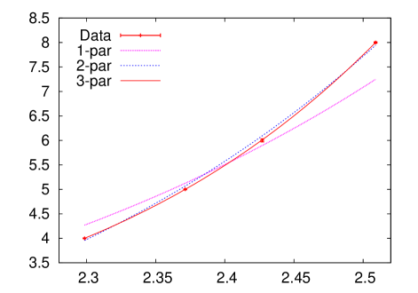
FIG. 1.: Uniform distribution: Impossible (left) and missing events (in the enlarged thickness of the right border).

B 2-parameter fits

The function (18) is now reduced to the form

$$y = N_{\tau}(\beta)\ =\ \frac{a_{2}}{f^{as}_{\lambda}(\beta)}\,\left(1+\frac{a_{1}}{\beta}\right)\,.$$ (27)

For the fit with two parameters we use the start values $a_{2}=0.0628450$ (as for $a_{1}$ before) and $a_{1}=-1.43424$. After six iterations we find convergence and the results

$$a_{1}=-1.5751\,(84)\,,\ a_{2}=0.07460\,(77)\,,\ \chi^{2}=117\,.$$ (28)

Running the fitting routine now just for the parameter $a_{1}$ by eliminating $a_{2}$ in the described way, we find the results (28) after four iterations. In particular, also the error bar of $c_{0}$, now calculated via Eq. (16), agrees with the error bar of $a_{2}$.

Clearly the $\chi^{2}$ is still too large to claim consistency between the fit and the data though the visible improvement is considerable. See the 2-par curve in Fig. 1.

C 3-parameter fits

We fit now to the full functional form (18). For the three parameter fit the previous starting values are re-shuffled $a_{2}\to a_{3}$, $a_{1}\to a_{2}$ and the additional starting value is taken to be $a_{1}=1$. Our Levenberg-Marquardt procedure needs 245 iterations for convergence and yields the values

$$a_{1} = 4.685\ (83)\,,~{}~{}a_{2}\ =\ -4.199\ (46)\,,$$ (29)

$$a_{3} = 0.395\ (30)\,,~{}~{}\chi^{2}=0.156\,,$$ (30)

which are rather different than the corresponding results $a_{3}\to a_{2}$ and $a_{2}\to a_{1}$ (28) of the 2-parameter fit.

Identical values (29), (30) are obtained after eliminating the normalization, here $a_{3}$, from the fit parameters used in the Levenberg-Marquardt iteration and we find a reduction of iterations from 245 to 12.

The $\chi^{2}$ is now small enough to signal consistency between the data and fit, although the 2-par and 3-par curves in Fig. 1 are hard to distinguish visually. Converting the $\chi^{2}$ of (30) into a goodness of fit one finds $Q=0.69$.

D 4-parameter fits

The aim is to perform the 4-parameter fit (23) for the data of Bhanot et al. (Table I). Using all four parameters, our first set of starting values,

$$a_{1}=-1.6\,,~{}~{}a_{2}=0.1\,,~{}~{}a_{3}=-1.0\,,~{}~{}a_{4}=0.8\,,$$

is chosen so that $a_{1}$ stays close to the 2-parameter fit result $-a_{1}=1/\nu=1.6185\,(2)$ from [3]. Running our Levenberg-Marquardt fit program on these initial values, it needs 391 iterations to converge and finds

$$a_{1} = -1.5981\,(31)\,,~{}~{}a_{2}\ =\ 0.77\,(39)\,,$$ (31)

$$a_{3} = -2.80\,(52)\,,~{}~{}a_{4}\ =\ 0.7917\,(61)\,,~{}~{}\chi^{2}=0.113\,,$$ (32)

where the $\chi^{2}$ can be converted into a goodness of fit $Q=0.74$.

Eliminating the normalization $a_{4}$ from the direct fitting parameters, convergence is reached after 58 iterations and we find identical estimates as before:

$$a_{1} = -1.5981\,(31)\,,~{}~{}a_{2}\ =\ 0.77\,(39)\,,$$ (33)

$$a_{3} = -2.80\,(52)\,,~{}~{}c_{0}\ =\ 0.7917\,(61)\,,~{}~{}\chi^{2}=0.113\,,$$ (34)

Noticeably, our example features a rugged landscape for $\chi^{2}$ as function of the parameters. With different starting values

$$a_{1}=-4.4\,,~{}~{}a_{2}=1.3\,,~{}~{}a_{3}=2.8\,,~{}~{}a_{4}=0.6$$

a minimum entirely different from the one above was found by accident. Running our Levenberg-Marquardt procedure on these starting values convergence is reached after 9 iterations and gives

$$a_{1} = -4.40\,(53)\,,~{}~{}a_{2}\ =\ 1.31\,(66)\,,$$ (35)

$$a_{3} = 2.80\,(52)\,,~{}~{}a_{4}\ =\ 0.61\,(31)\,,~{}~{}\chi^{2}=0.113\,.$$ (36)

Eliminating the normalization $a_{4}$ we find convergence after 8 iterations and the same results:

$$a_{1} = -4.40\,(53)\,,~{}~{}a_{2}\ =\ 1.31\,(66)\,,$$ (37)

$$a_{3} = 2.80\,(52)\,,~{}~{}a_{4}\ =\ 0.61\,(31)\,,~{}~{}\chi^{2}=0.113\,.$$ (38)

Either set of parameters fits the data perfectly well in their range, while the different fits function diverge quickly out of this range, i.e., for larger lattices.

IV Conclusion and Outlook

This paper shows that we can exclude the multiplicative normalization of a fitting function from the variable parameters of a $\chi^{2}$ minimization and include it into the fitting function (it still counts when it comes to determining the degrees of freedom). Our simple examples show that this works well, reducing the number of iterations.

The code discussed in appendix A shows that there is no extra work involved for the user. Once the general, application independent, code is set up, the subroutine which the user has to supply has one parameter less than the one needed for the usual Levenberg-Marquardt fitting procedure (compare the reduction from subg_la3su2.f to suby_la3su2.f). Besides, it is useful to have alternatives at hand when one is trying to find convenient initial values.

Finally, there may be interesting applications, which cannot be easily incorporated into conventional fitting schemes. For instance, there are situations where distinct data sets are supposed to be described by the same function with different multiplicative normalizations. An example is scale setting in lattice gauge theories [11]. The method of this paper can then be used to eliminate all multiplicative constants from the independent parameters of the fit so that one can consolidate all data sets into one fit. This application will be pursued elsewhere.

A Fortran implementation

For a limited time the Fortran code can still be downloaded as archive FITM1.tgz from the authors website at

http://www.hep.fsu.edu/~berg/research/research.html .

After downloading the FITM1.tgz file, it unfolds under

$$\rm tar\ -\!zxvf\ FITM1.tgz$$

into a tree structure with the folder FITM1 at its top. On the next level there are two subfolders examples and libs. To reproduce the results of section III go to the examples folder, where one finds the subfolders 1par, 2par, 3par and 4par.

Each of these subfolders contains two Fortran programs, $n$gfit.f and $n$gfitm1.f, where $n=1,2,3$ or 4 denotes the number of parameters. Both programs are ready to be compiled and run, say with ./a.out$>$a.txt. The thus produced results should agree with those found in the text file a$n$.txt and a$n$m1.txt. In addition graphical output is created. Type

$$\rm gnuplot\ gfit.plt$$

to see the plots (a gnuplot driver gfit.plt is located in each folder).

The programs read data and starting values from files named fort.10. For the $n=4$ case there are two sets, bhanot1.dat and bhanot2.dat, which differ by the initial values and the desired one has to be copied on fort.10 before the run.

With exception of 1gfitm1.f, which is a special case discussed at the end of this appendix, the programs rely on our Levenberg-Marquardt subroutine fitsub to find the minimum of $\chi^{2}$. This subroutine, is transferred after the end statement of each main program by an include statement into the code,

      include ’../../libs/fortran/fitsub.f’

and in the same way this is done for all others routines needed. These include statements allow for easy tracking of the location of the source code of each routine.

The crucial difference between the two main programs is: $n$gfit.f calls fitsub for nfit=$n$ parameters, but $n$gfitm1 calls it for nfit$=$n$-1$ parameters. This is achieved by feeding distinct subroutines subg into fitsub, which define the fitting functions and their derivatives with respect to the nfit parameters. For instance, for the 3-parameter case the subroutine used by the run of 3gfit.f is subg_la3su2.f as listed here:

      subroutine subg(x,a,yfit,dyda,nfit)
c BB May 20 2015. User provided subroutine
c for a 3-parameter fit of the pure su2 scale,
c yfit=a3*(1+a2/x+a1/x**2)/flasu2(x,2) with x=beta
c and flasu2(x,2) the asymptotic su2 scaling
c function (yfit has the dimension of a length).
      include ’../../libs/fortran/implicit.sta’
      include ’../../libs/fortran/constants.par’
      dimension a(nfit),dyda(nfit)
      if(nfit.ne.3) stop "subg_la3su2: nfit.ne.3."
      x2=x**2
      flasu2=fla(x,itwo)
      dyda(3)=(one+a(2)/x+a(1)/x2)/flasu2
      yfit=a(3)*dyda(3)
      dyda(2)=(a(3)/x)/flasu2
      dyda(1)=(a(3)/x2)/flasu2
      return
      end

The 3gftim1.f program and all other $n$gfitm1.f programs, but $n$=1, include subgfitm1.f with the following code:

      subroutine subg(xx,aa,yfit,dyda,nfit)
c BB May 20 2015. Generic routine for least square
c fit with one parameter less. Input needed: User
c provided subroutine suby for unnormalized fit
c function and its derivatives with respect to
c its parameters.
      include ’../../libs/fortran/implicit.sta’
      include ’../../libs/fortran/constants.par’
      include ’../../libs/subs/common_fitting.f’
c For this routine the common transfers x,y,ye.
      dimension aa(nfit),dyda(nfit)
      call chi2dcda(ndat,nfit,x,y,ye,aa,dcda,c0)
      call suby(xx,aa,yy,dyda,nfit)
      yfit=c0*yy
      do i=1,nfit
        dyda(i)=c0*dyda(i)+dcda(i)*yy
      enddo
      return
      end

Here the call to suby defines the user supplied function and its derivatives as the subg routines do for the $n$gfit.f programs. The suby routines replace the normalization parameters by the number one. For our example above subg_la2su2.f becomes suby_la2su2.f given by

      subroutine suby(x,a,y,dyda,nfit)
c BB may 20 2015. User provided fit function
c y=(1+a2/x+a1/x**2)/flasu2(x,2) and derivatives.
      include ’../../libs/fortran/implicit.sta’
      include ’../../libs/fortran/constants.par’
      dimension a(nfit),dyda(nfit)
      if(nfit.ne.2) stop "suby_la3su2: nfit.ne.2."
      x2=x**2
      flasu2=fla(x,itwo)
      y=(one+a(2)/x+a(1)/x2)/flasu2
      dyda(2)=(one/x)/flasu2
      dyda(1)=(one/x2)/flasu2
      return
      end

This it the only routine, which the user has to define for the reduced fitting procedure. The chi2dcda routine called in subgfitm1.f is generic for all these fits and calculates $c_{0}$ (7) and its derivatives (13) as defined in section II with the following code:

      subroutine chi2dcda(n,nf,x,y,ye,a,dcda,c0)
c BB May 20 2015. Determination of the normalization
c constant c0 for chi2 fit of data y_i with the fit
c function c0*f. Then, in dcda the derivatives of
c c0 with respect to the fit parameters.
c Input: data arrays x(n),y(n),ye(n),
c        parameter array a(nf).
c Output: dcda(nf), c0.
c        variable fit parameters a(nf).
      include ’../../libs/fortran/implicit.sta’
      include ’../../libs/fortran/constants.par’
      parameter(mf=30) ! maximum number parameters.
      dimension drda(mf),dsda(mf),dfda(mf),a(nf),
     &  dcda(nf), x(n),y(n),ye(n)
      if(nf.gt.mf) stop "chi2dcda: nf.gt.mf."
      r=zero
      s=zero
      do j=1,nf
        drda(j)=zero
        dsda(j)=zero
      enddo
      do i=1,n
        call suby(x(i),a,f,dfda,nf)
        ye2i=one/ye(i)**2 ! 1/(error bar squared).
        ri=f*ye2i
        r=r+y(i)*ri     ! iterate r.
        s=s+f*ri        ! iterate s.
        addy=y(i)*ye2i
        addf=two*ri
        do j=1,nf
          drda(j)=drda(j)+addy*dfda(j)
          dsda(j)=dsda(j)+addf*dfda(j)
        enddo
      enddo
      c0=r/s
      do j=1,nf
        dcda(j)=(s*drda(j)-r*dsda(j))/s**2
      enddo
      return
      end

An extension of this routine, chi2c0eb.f, calculates also the variance (16) of $c_{0}$ and needs on input the covariance matrix of the parameters $a_{1},\dots,a_{n-1}$.

Finally, the program 1gfitm1.f is a special case, because the fitsub routine does not work for nfit=0 parameters. Actually, it is not needed at all in this case and becomes replaced by a variant of the chi2dcda.f routine: chi2c0.f calculates $c_{0}$ (7) and its error bar, now according to Eq. (9) instead of (16).

REFERENCES

- [1] K. Levenberg, Qty. Appl. Math. 2 (1944) 164.
- [2] D.W. Marquardt, SIAM 11 (1963) 431.
- [3] B.A. Berg, Markov Chain Monte Carlo Simulations and Their Statistical Analysis, World Scientific, Singapore 2004.
- [4] B. Lucini, M. Teper and U. Wenger, JHEP 1 (2004) 61.
- [5] The and parameters are some of the corrections contained in the functional form proposed by A. Bazavov, B.A. Berg and A. Velytsky, Phys. Rev. D 74 (2006) 014501.
- [6] D.J. Gross and F. Wilczek, Phys. Rev. Lett. 30 (1973) 1343.
- [7] D. Politzer, Phys. Rev. Lett. 30 (1973) 1346.
- [8] D.R.T. Jones, Nucl. Phys. B 75 (1974) 531.
- [9] W. Caswell, Phys. Rev. Lett. 33 (1974) 244.
- [10] G. Bhanot, R. Salvador, S. Black, P. Carter and R. Toral, Phys. Rev. Lett. 59 (1987) 803.
- [11] For a review see: R. Sommer, POS (Lattice 2013) 015.