Asymptotics for Critical First Passage Percolation
Abstract.
We consider first-passage percolation on with i.i.d. weights, whose distribution function satisfies . This is sometimes known as the “critical case” because large clusters of zero-weight edges force passage times to grow at most logarithmically, giving zero time constant. Denote as the passage time from the origin to the boundary of the box . We characterize the limit behavior of by conditions on the distribution function . We also give exact conditions under which will have uniformly bounded mean or variance. These results answer several questions of Kesten and Zhang from the ’90s and, in particular, disprove a conjecture of Zhang ([zhang1999double]) from ’99. In the case when both the mean and the variance go to infinity as , we prove a CLT under a minimal moment assumption. The main tool involves a new relation between first-passage percolation and invasion percolation: up to a constant factor, the passage time in critical first-passage percolation has the same first-order behavior as the passage time of an optimal path constrained to lie in an embedded invasion cluster.
Key words and phrases:
First passage percolation; critical percolation; correlation length; invasion percolation; central limit theorem1. Introduction
1.1. The model
Consider the integer lattice and denote by the set of nearest-neighbor edges. Given a distribution function with , let be a family of i.i.d. random variables (edge-weights) with common distribution function . In first-passage percolation, we study the random pseudo-metric on induced by these edge-weights.
The model is defined as follows. For , a (vertex self-avoiding) path from to is an alternating sequence , where the ’s, , are distinct vertices in which are different from or , and , ; is an edge in which connects and . If , the path is called a (vertex self-avoiding) circuit. For a path , we define the passage time of to be . For any , , we define the first-passage time from to by
For , write for and similarly for . A geodesic is a path from to such that .
It is a consequence of the sub-additive ergodic theorem that if for all then there exists a constant , called the time constant, such that
where . It was shown by Kesten [kesten1986aspects, Theorem 6.1] that
| (1.1) |
where is the critical probability for Bernoulli bond percolation on . Therefore the time constant does not provide much information if .
In [zhang1995supercritical, Eq. 3], Y. Zhang introduced the following random variable
where , , and is the sup-norm. By monotonicity, exists almost surely. It was shown in [zhang1995supercritical, p. 254] that if and has all moments, then for any , one has , and hence in particular almost surely. Also, it is easy to see that if , then almost surely. Then a natural question arises: how about ?
In [zhang1999double], Zhang proved that for , it is possible to have or almost surely when (note that by the Kolmogorov zero-one law, either almost surely or almost surely). More specifically, he introduced the following two distributions. For , set
and for , set
Zhang showed in [zhang1999double, Theorem 8.1.1] that if is sufficiently small then almost surely. He also made the following conjecture (see [zhang1999double, p. 146]):
Conjecture 1.1 (Zhang).
The quantity is finite.
Moreover, Zhang showed in [zhang1999double, Theorem 8.1.3] that if , then almost surely.
The critical case of first-passage percolation is quite different from the standard one and requires different techniques. For example, the model is expected to retain rotational invariance in the limit [yao2014law], whereas the usual first-passage model has lattice dependent and distribution dependent asymptotics. For this reason, analysis of the critical case relies on detailed estimates from critical and near-critical percolation (for instance, see [sapozhnikov2011incipient, jarai2003invasion, van2007size]). The main new insight of our work is that the behavior of passage times is closely related to a “greedy” growth algorithm called invasion percolation, and that optimal paths constrained to lie in the invasion cluster have the correct first-order growth. This relation allows us to derive necessary and sufficient conditions on the edge-weight distribution to have diverging mean or variance for passage times (Theorems 1.2 and 1.5), and these results can be seen as finer versions of Kesten’s condition (1.1) for . Furthermore, we can derive a type of universality: for any edge weights for which the passage-time variance diverges, one has Gaussian fluctuations (see Theorem 1.6).
Constants in this paper may depend on the distribution function and other fixed parameters such as , and . However, constants do not depend on or . We use to denote temporary constants whose meaning may vary, while we use notation like to denote the permanent constants. For example, denotes the constant in Lemma 3.1.
1.2. Main results
In this paper, we will give an exact criterion for (see Corollary 1.3 below) and consequently provide a negative answer to Conjecture 1.1. Furthermore, we will derive limit theorems for the sequence . From now on, suppose that and that . Furthermore, define
and
| (1.2) |
1.2.1. Behavior of the mean
We begin with bounds on .
Theorem 1.2.
(i) Assume that . There exists such that
(ii) There exists such that
Remark 1.
Note that if and only if for some , where is the minimum of four i.i.d. random variables distributed as . The moment condition in Theorem 1.2 is nearly optimal since, if then, by bounding below by the minimum of the edge-weights on edges incident to , one has for .
Remark 2.
The above theorem concerns the passage time from the point to the set . In Section 5.4, we derive asymptotics for point-to-point passage times for .
As a corollary, we have an exact criterion for finiteness of .
Corollary 1.3.
For any , one has almost surely if and only if .
We will now apply the above results to and , the distributions defined by Zhang. The proof follows by a direct computation and the previous corollary.
Corollary 1.4.
The following statements hold.
-
(1)
almost surely for any , and so . In particular, Conjecture 1.1 is false.
-
(2)
almost surely if and only if .
Remark 3.
Zhang asked in [zhang1999double, p. 145] if, under the assumption for all , does almost surely imply that ? The answer is yes by combining all the above results.
1.2.2. Behavior of the variance and limit theorems
Now we consider .
Theorem 1.5.
Assume that .
(i) There exists such that
(ii) There exists such that
By Corollary 1.3, when we have as , . The next theorem gives more information about the limit of in this case.
Theorem 1.6.
Suppose and .
(i) If , then there is a random variable with and such that as
(ii) If , then as
1.3. Relations to previous work
First-passage percolation has been studied since its introduction by Hammersley and Welsh [hammersley1965first] in the ’60s, but most work has focused on the non-critical case, where . There, the passage time from to a vertex grows linearly in , and many results have been proved, including shape theorems, large deviations, concentration inequalities and moment bounds. We refer the reader to the surveys [grimmett2012percolation, blair2010first]. The supercritical case, where is easier to analyze, since there is almost surely an infinite cluster of edges with passage time 0, and so distant vertices need only to travel to the infinite cluster to reach one-another. This produces passage times that are of order one as .
The critical case, where , is considerably more subtle. It is expected (though only proved in two dimensions or high dimensions) that there is no infinite cluster of -open edges (that is, edges with passage time 0 in this case). However, clusters of -open edges occur on all scales, giving, for example, infinite mean size for the -open cluster of the origin. This means that two distant points can be connected by a path which uses mostly zero-weight edges, and this path may be able to find lower and lower edge weights as it moves further into the bulk of the system. Therefore to characterize passage times, one should understand the balance between the number of edges on each scale with low weights and the number of paths that can access them.
Kesten proved in [kesten1986aspects, Theorem 6.1] that the time constant is zero in the critical case, implying that as . This result was sharpened by L. Chayes [chayes1991critical, Theorem B], who showed that for any , almost surely. In [kesten1993speed, Remark 3], Kesten claimed that in fact Chayes’s argument can be extended to for large almost surely. These results go some way to quantify asymptotics of the passage time in the critical case for general dimension.
More progress has been made in the critical case in two dimensions, due to a more developed theory of Bernoulli percolation on planar lattices. It was shown by Chayes-Chayes-Durrett in [chayes1986critical, Theorem 3.3] that if is Bernoulli (0 or 1 with probability 1/2) then the expected passage time grows logarithmically, obeying . In this Bernoulli case, the passage time between and can be represented as the maximum number of disjoint -closed circuits separating and , as every -closed edge on a geodesic contributes passage time 1. Recently, Yao [yao2014law] has shown a law of large numbers on the triangular lattice, using the conformal loop ensemble of Camia and Newman.
Our work was motivated by that of Zhang in ’99, who showed that critical FPP can display “double behavior.” That is, he showed that there exist distributions with for which the passage time diverges as , and those for which the passage time remains bounded. Intuitively, bounded passage times come from those distributions which have significant mass near zero, so that long paths can find more and more low weights as they move away from , producing infinite paths with finite passage time. Zhang asked many questions about this case, in particular which distributions have which of the two behaviors. One main point of our work is Theorem 1.3, which gives an exact criterion that this passage time remains bounded if and only if . Our proof involves a new relation to a model called invasion percolation, and it turns out that optimal paths in the invasion cluster have passage time of the same order as geodesics in FPP. (See the next section for more details.) This theorem allows us to answer Zhang’s questions in the two-dimensional case.
The other motivation for our work is that of Kesten and Zhang in ’97. They also considered the critical case in two dimensions and proved central limit theorems for for a certain class of distributions. Precisely, they showed that if for some , , and there exists a constant such that , then the sequence satisfies a Gaussian central limit theorem: there exists a sequence such that
and
It is important to notice that the condition gives a positive lower bound for the passage time of non-zero weight edges. Kesten and Zhang do not address any distributions with mass near zero, though they do remark about the double behavior of such distributions.
The second part of our paper, on limit theorems and variance estimates, completes the picture started by Kesten and Zhang. Theorems 1.5 and 1.6 (ii) require only that and a weak moment condition on (lower than that of Kesten and Zhang) to deduce that the variance of diverges and that a Gaussian CLT holds. This result on the CLT shows that in the critical case, no other limiting behavior is possible, in contrast to the subcritical case, where the variance is expected to be of order with a non-Gaussian limiting distribution (see [kardar1986dynamic]). Theorem 1.6 (i) also addresses the intermediate case, where the mean of diverges but the variance converges. Here, the centered sequence is tight and converges to a non-trivial limit. We do not know an exact form for this limit, and it is unlikely to be explicit since its variance depends heavily on weights of edges near the origin.
2. Setup for the proof
Zhang’s proof in [zhang1999double, Theorem 8.1.1] that has all moments used a comparison to a near-critical percolation model introduced in [chayes1987inhomogeneous] by Chayes-Chayes-Durrett. Their model is a version of an incipient infinite cluster, a term used by physicists to describe large (system-spanning) percolation clusters at criticality. We will, however, need finer asymptotics that are obtained by comparison with a different near-critical model, invasion percolation. Though it has no parameter, it tends on large scales to resemble Bernoulli percolation at criticality. We describe the model of invasion percolation in Section 2.1. We also recall some known facts about Bernoulli percolation in Section 2.2.
We will couple the first-passage percolation model on with invasion percolation and Bernoulli percolation. To describe the coupling, we consider the probability space , where , is the cylinder sigma-field and , where each is an uniform distribution on . Write . Define the edge weights as for .
2.1. Invasion percolation
If an edge has endpoints and , we write . For an arbitrary subgraph of , define the edge boundary by
Define a sequence of subgraphs as follows. Let . If is defined, we let , where is the edge with , and let be the graph induced by . The graph is called the invasion percolation cluster (at time infinity).
Invasion percolation is coupled with the first-passage percolation model since we have defined . They can also be coupled with Bernoulli percolation as follows. For each and , we say that is -open in if and otherwise we say that is -closed. If there is a -open path from a vertex set to a vertex set then we write that by a -open path. The collection of -open edges has the same distribution as the set of open edges in Bernoulli percolation with parameter .
To use this coupling, we need the notion of the dual graph. Let and . For , we write . For , we denote the its endpoints (left respectively right or bottom respectively top) by , . The edge is called the dual edge to e and its endpoints (bottom respectively top or left respectively right) are denoted by and . For , is defined to be . An edge is declared to be -open in when is, and -closed otherwise.
We note the following relations between invasion percolation and Bernoulli percolation:
-
•
With probability one, if is a vertex of and by a -open path, then .
Proof: If is not in then we can find (on a -open path from to ) such that is -open. But then for all large . By the definition of the invasion algorithm, this means that for large , each edge added to the invasion is -open, and from this we can build an infinite -open path. This contradicts the fact that there is almost surely no infinite -open cluster [kesten1980critical, Theorem 1].
-
•
For , let be defined as
(2.1) where is the set of edges with both endpoints in . Then
(2.2) where
Here the diameter of a set is .
Proof: Take with . At the moment that is added to the invasion cluster, the graph has edge boundary all of whose edges are -closed, and so are -closed. However, from the edge boundary, we can extract a dual circuit around 0 that contains , by [grimmett1999percolation, Proposition 11.2]. This circuit then has diameter at least .
2.2. Correlation length
A central tool used to study invasion percolation is correlation length, and we take the definition from [kesten1987scaling, Eq. 1.21]. For and , let
where a -open left-right crossing of means a path in with all edges -open which joins some vertex on to some vertex on . For and , we define
is called the correlation length. It is known (see [kesten1987scaling, Eq. 1.24]) that there exists such that for all , the ratio is bounded away from 0 and as . We will write for simplicity. For , define
| (2.3) |
We now note the following facts.
-
•
By [jarai2003invasion, Eq. (2.10)] there exists such that for all we have
(2.4) -
•
There exist such that for all ,
This is a consequence of [nolin2008near, Prop. 34] and a priori estimates on the four-arm exponent. In particular, putting , there exist such that for
(2.5) We may and will always assume .
-
•
From [van2008random, Eq. 9] and (2.2), There exist such that for all and ,
(2.6) -
•
By the RSW theorem (see [grimmett1999percolation, Section 11.7]), there exists such that for all ,
(2.7)
2.3. Sketch of proofs
The central tool used to prove our theorems is Lemma 3.1, which is a moment bound on annulus passage times. We first describe the idea of its proof. Consider all paths between and which lie in the invasion cluster and . Let be such a path which minimizes the passage time. Then Lemma 3.1 gives an upper bound on the -th moment of the sum of edge-weights for edges in which lie in any annulus (that is, , where is defined in (3.1)).
The passage time of gives an upper bound for the passage time from to , and is in many ways is a nicer path than the actual geodesic using the edge-weights . Once the invasion has reached the boundary of , all of its edges (from that point on) are likely to be nearly -open (that is, from (2.1) is of order ), and so the edges in outside of will have passage time bounded above by . By bounding above with (2.5), each edge has passage time bounded by , where is defined in (3.2). Unfortunately we only know this behavior of with high probability, so we need to decompose the probability space over different values of using an idea of A. Járai [jarai2003invasion].
The above heuristic gives
The reason is that the only edges which contribute to the passage time of are those which are -closed. In Lemma 3.2, we show that each such edge has “4-arms.” That is, they have the property that (a) their weight is between and , (b) they have two disjoint -open arms to distance and (c) they have two disjoint -closed arms to distance . Fortunately all moments of the number of such points in an annulus were bounded in the study of invasion percolation in [damron2011outlets] (see Lemma 3.3 below), so we can conclude.
2.3.1. Idea of the proof of Theorem 1.2
The proof of (ii) follows that of Zhang [zhang1999double, Theorem 8.1.2]. The proof of (i) follows immediately from Lemma 3.1. Indeed, to find the upper bound for , we simply use the inequality
where, as above, each is the time that spent in the annulus . Applying the annulus moment bounds from Lemma 3.1 gives (i).
2.3.2. Idea of the proof of Theorem 1.5 and 1.6
To study the variance and limit theorems, we follow the strategy of Kesten-Zhang [kesten1997central]. Instead of dealing with directly, we consider , where is the innermost -open circuit in an annulus for surrounding . It can be shown that these two variances are closed to each other. The variance bounds for are stated in Theorem 5.1 and the CLT is stated in Theorem 5.2.
If we write as a sum of martingale differences
over a filtration , then , so it suffices to bound the ’s. The idea of Kesten-Zhang was to take to be generated by the edge-weights for edges on and in the interior of , and they proved an alternate representation for such ’s (see Lemma 5.3 (ii)). With this same choice, we can use the moment bounds in Lemma 3.1 to prove moment bounds on the ’s in Lemma 5.5. We emphasize that in fact, as a result of the representation in Lemma 5.3 (ii), does not depend on .
To prove the CLT for , we apply McLeish’s CLT, which we state as Theorem 5.7. We verify its conditions using the fact that the ’s can be shown to be strongly mixing (see Lemma 5.8), Along with moment bounds for the ’s given in Lemma 5.5 (which use our main moment bounds on annulus times), we can conclude the CLT in the case that the variance of diverges. This will prove (ii) in Theorem 1.6. For (i), if the variance does not diverge, then by the martingale convergence theorem, will converge to some random variable . Using a stronger comparison to given in Lemma 5.10 allows to complete the proof.
3. Moment bounds for annulus times
In this section, we prove the main lemma of the paper, Lemma 3.1. It serves to bound certain annulus passage times through the invasion cluster.
Recall that we denote as the invasion percolation cluster using the weights . Define and for . Note that and for . For any path , define for
| (3.1) |
For , let be a path such that
Note that . Recall from (2.5). For simplicity of notation, define
| (3.2) |
Note that is only defined when the argument of is strictly less than , and this will be guaranteed by the condition in the lemma below.
The main goal of this section is to prove the following lemma.
Lemma 3.1.
Recall the definition of from (1.2) and suppose .
(i) For all and integers , we have .
(ii) Given any and , there exist and , such that for all we have
Remark 5.
We begin with a definition from [damron2011outlets]. For , , and , let be the event that
-
(a)
is connected to by two vertex disjoint -open paths,
-
(b)
is connected to by two vertex disjoint -closed dual paths, and
-
(c)
.
Here . Let be the number of edges in such that occurs; that is,
Lemma 3.2.
Let be as in (2.1). For all and we have
Proof: Suppose for some . Define, for and
Since and , we have . Then it is sufficient to show
| (3.3) |
Let be -closed. As and , is -open. Note that there exist disjoint paths , such that is a -open path joining to and is a -open path joining to . (This holds because is invaded but .)
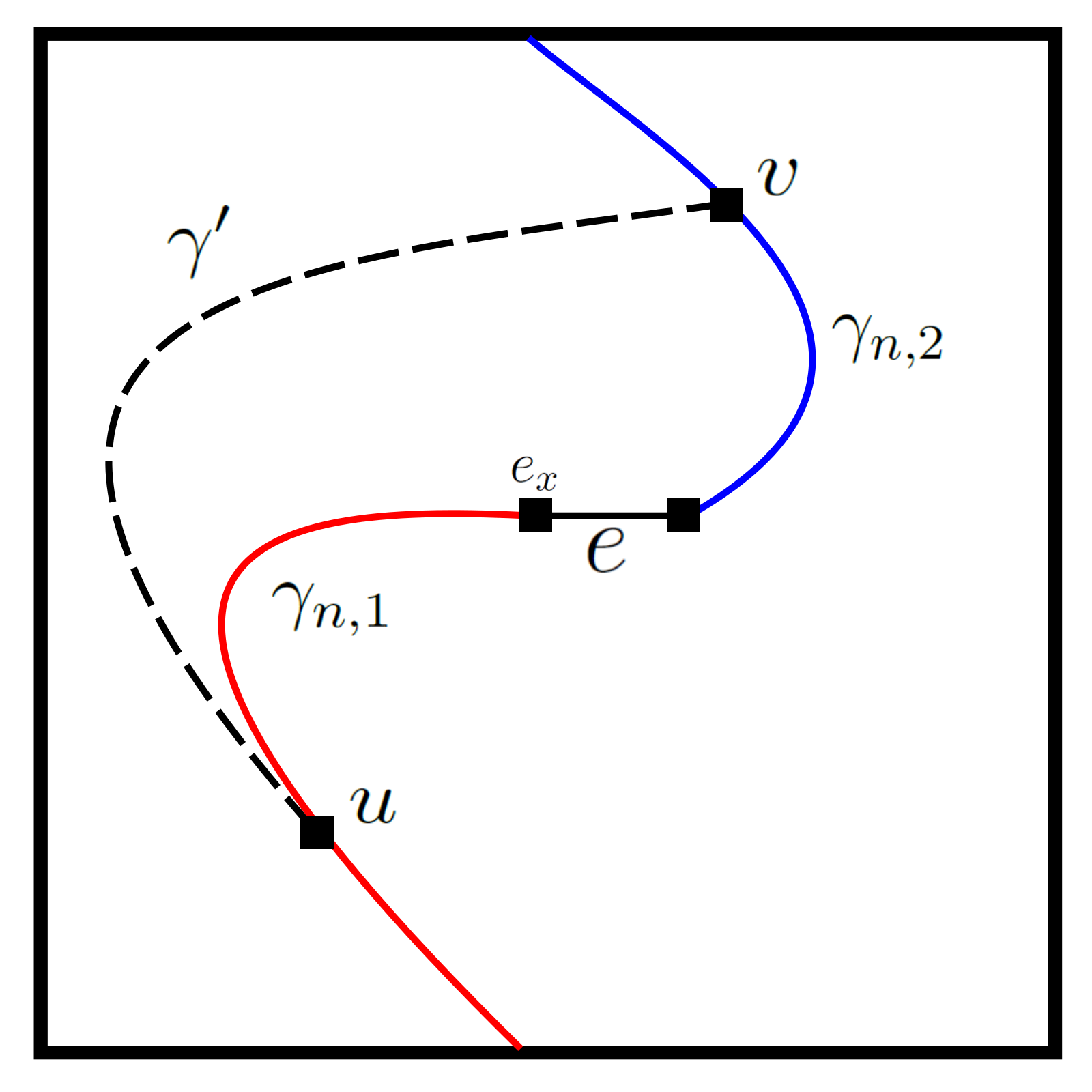
For an illustration of the following argument, see Figure 3.1. If by a -open path in , and if we let and be such that via , then every vertex in the path is in (see the first bulleted fact in Section 2.1). Therefore . Now let be the path which connects and via , to via and to via . Then is in and has at least one -closed edge less (namely ) than . Furthermore, each -closed edge of is a -closed edge of , and this implies , contradicting the minimality of . Hence by a -open path in . Note that by duality, exactly one of the following will happen:
-
(1)
and are connected to by two disjoint -closed dual paths, which are also disjoint from ;
-
(2)
there is a -open path connecting and in .
So the first event must happen and thus occurs. This completes the proof of Lemma 3.2.
Next we bound the moments of using a result from [damron2011outlets, Lemma 5.1].
Lemma 3.3.
There exists such that for all , and integers
Proof: The first inequality immediately follows from the definition of . In [damron2011outlets, Lemma 5.1], it was shown that there exists such that if , and , then for all integers ,
Taking completes the proof.
The next lemma will be used to control moments of when is large. Define
| (3.4) |
Lemma 3.4.
Suppose for some . Define and for . Then for all integers and , one has . In particular, for any fixed , there exists such that for all integers , we have
Proof: Note that for all . Then we have
| (3.5) |
In order to bound the tail probability of , we need to bound when is close to one. By (2.2), for any , implies that there exists a -closed dual circuit surrounding the origin with diameter at least . Such a dual circuit must have length at least , for . For any even , observe that since dual circuits around the origin with length must intersect the line , the total number of such circuits is bounded by . Each of these dual circuit is -closed with probability . Therefore when we have
where the second inequality uses the facts that and the value of will be specified later. Define and . Combining (3.5) and the above bound, when we have and
Since , taking we have
Therefore, using the relation , we have
This proves the statement that .
Next, when and , taking in the above proof, we have where . Then
which gives the expression of .
Now we are ready to prove Lemma 3.1.
Proof of Lemma 3.1: First we prove part (i). Recall from (3.4). Since and for , we have
| (3.6) |
Since for any , there exists such that . Recall from Lemma 3.4. For all we have, . Thus by Lemma 3.4, and (i) is proved.
Next, we prove (ii). The constants are from (2.5). We will perform a decomposition for introduced by Járai [jarai2003invasion, p. 319] using iterated logarithms. Define and for such that it is well-defined. For , let
Denote, for ,
where is so large that
| (3.7) | |||
| (3.8) | |||
| (3.9) |
Given , let be the smallest integer such that for all ,
| (3.10) |
The reason for the above choices will be clear as the proof proceeds. We assume for the rest of the proof. By Lemma 3.4, the third condition in the above display implies that , and combining this with (3.6) we have for all ,
| (3.11) |
Note that are well-defined as long as . We decompose as follows:
| (3.12) |
By (2.4) and the fact that , for and ,
Then applying Lemma 3.2 and Lemma 3.3, for all , and ,
| (3.13) |
By (3.10) we have for and ,
| (3.14) |
Then by (2.5) we have
| (3.15) |
Applying (2.4) and (3.15) in (3.13), we have for and with ,
| (3.16) |
where . Now we bound the sum in (3.12), starting with the last term. Applying (3.16) with and , we have for and ,
| (3.17) |
For the first term in (3.12), applying Cauchy-Schwarz inequality, (3.11) and (2.6), for ,
| (3.18) |
For the second term in (3.12), applying Cauchy-Schwarz inequality, (3.16) with , and (2.6), we have for and ,
| (3.19) |
Then combining (3.18), (3.19), (3.17) and using the definition of in (3.8) and (3.9), there are such that for ,
Using [van2007size, Eq. 2.16] which says is uniformly bounded in , we complete the proof of Lemma 3.1.
4. Study of the mean
4.1. Proof of Theorem 1.2
First we prove an elementary lemma.
Lemma 4.1.
Let , , be a positive non-increasing function. Fix and integers . Then there exist constants such that for all ,
Proof: It suffices to prove the lemma for . If , then , and for each there are at most such integer . Therefore
As , we obtain
and this completes the proof.
Now we prove Theorem 1.2.
4.2. Proof of Corollary 1.3
To prove Corollary 1.3, we need the following definition from [zhang1999double, p. 146]. Given two distribution functions and , we say that if there exists such that for all . By [zhang1999double, Theorem 8.1.4], if almost surely and if , then almost surely. (This is in fact provable in general dimensions, though Zhang only gave a proof for .)
Proof of Corollary 1.3: Suppose that . Let be arbitrary, and let be a distribution function such that on and there exists such that . Note that we still have and has all moments. By Theorem 1.2(i), almost surely. Since , we have almost surely.
Now suppose that . This implies that for from (2.5). For , write
and . For , define and compute by Cauchy-Schwarz, (2.7) and independence of the ’s:
By the Paley-Zygmund inequality (second moment method), we can find such that for all ,
Therefore
Because for all , this implies that with probability at least . Since, almost surely or almost surely, this completes the proof.
5. Study of the variance
In this section, we prove Theorems 1.5 and 1.6. The main tool is the construction of a martingale introduced in [kesten1997central]. We start with some definitions.
Define the annuli
For a vertex self-avoiding circuit in , write for the graph induced by all the vertices in that are either on or in the interior of . Define
| (5.1) |
Note that . Write to emphasize the underlying weights . Denote as the smallest -open circuit in : precisely,
| (5.2) |
Define
| (5.3) |
By definition we have . For , we have , thus forms a filtration. Denote and . Instead of , we first try to study . Write
Then is an -martingale increment sequence. Thus
| (5.4) |
Theorem 5.1.
Let be as defined in (1.2).
(i) If , then there exists such that for ,
(ii) There exists such that for ,
Theorem 5.2.
Assume that . Further assume . Then as ,
We will first prove Theorem 5.1 in Section 5.1. Next in Section 5.2 we prove the CLT stated in Theorem 5.2. Finally, in Section 5.3, we control the difference between and for and prove Theorems 1.5 and 1.6.
5.1. Proof of Theorem 5.1
Because of (5.4), we first study bounds on the moments of . An important ingredient is an alternative formula for which was proved in [kesten1997central, Lemma 2], and we state it as part (ii) in the following lemma. Denote as another copy of the probability space . Let denote the expectation with respect to , and denote a sample point in . Denote , and for the quantities defined as in the previous sections, but with explicit dependence on . Define , or equivalently,
We need the following results, which are [kesten1997central, Lemma 3] and [kesten1997central, Lemma 2].
Lemma 5.3 (Kesten-Zhang).
(i) There exists such that for all integers ,
(ii) For all , does not depend on . Precisely,
Sometimes we will write instead of or when the meaning is clear from the context. The following lemma is a consequence of Lemma 3.1.
Lemma 5.4.
Assume .
(i) For any and , there exist and such that for all and ,
(ii) For any , there exists a constant such that for all and ,
Proof: Take . Since provides a specific path connecting the inner and outer boundaries of the annulus, we have . Therefore, by applying Jensen’s inequality and Lemma 3.1 for , we have
This proves (i). To prove (ii), if , by Lemma 3.1 (parts (i) and (ii) combined), for all we have for some constant . Using this fact in the above bound proves (ii).
We now show how the above lemma implies bounds on moments of the ’s.
Lemma 5.5.
Assume .
(i) For any and , there exist and such that for all ,
(ii) For any and , we have .
Proof: First we prove (i). Using the fact that and Lemma 5.3 (ii), we have
By Jensen’s inequality, we have
| (5.5) |
First we give an upper bound for the second term. Recall from Lemma 5.5. Fix , and estimate for ,
| (5.6) |
where the fourth line uses the Cauchy-Schwarz inequality, the fifth line uses Lemma 5.4 with and Lemma 5.3(i), and in the fifth line . Therefore
| (5.7) |
By Lemma 5.3(i) , so we complete the bound on the second term in (5.5). To bound the first term in (5.5), similar to (5.6), applying Cauchy-Schwarz inequality, we have for ,
| (5.8) |
Combining (5.5), (5.7) and (5.8), we complete the proof of Lemma 5.5 (i).
The proof of part (ii) can be done in exactly the same way, using Lemma 5.4 (ii).
The next lemma gives a lower bound for .
Lemma 5.6.
Proof: Recall the expression of in Lemma 5.3(ii) and the filtration in (5.3). The goal of the proof is to construct an event with uniformly in such that for ,
| (5.9) | |||
| (5.10) |
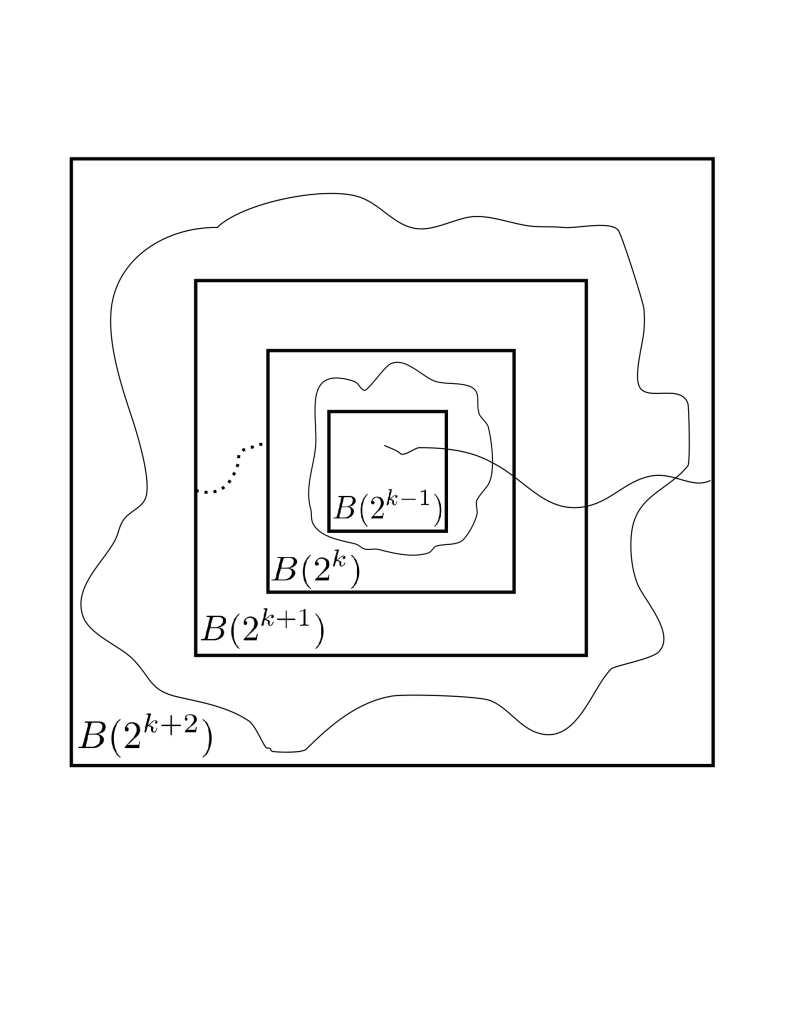
where is a constant. We start by defining the event to be the intersection of the following events (see Figure 5.1):
-
(1)
There exists a -open circuit around in .
-
(2)
There exists a -open circuit around in .
-
(3)
There exists a -open left-right crossing of .
-
(4)
There exists a dual -closed left-right crossing of .
By the RSW Theorem ([grimmett1999percolation, Sect. 11.7]), each of the above events has probability bounded from below for all . The events (1), (2) and (3) are all non-increasing, and they are jointly independent from (4). Therefore applying independence and the FKG inequality, there exists a constant such that for all . Now consider a new event :
-
There exists a -open left-right crossing of .
Define the event to be the intersection of the events (1),(2), (4) and . Then , and therefore . By definition, we have for . To see (5.10), recall the definition of in (2.3). Let be the event
From (2.7), let be such that for all . When and , since every path between and must cross the -closed dual circuit defined in and then cross , we have for
where the last inequality follows from (2.5). This proves (5.10) and therefore we have , completing the proof of Lemma 5.6.
Now we complete the proof of Theorem 5.1.
5.2. Proof of Theorem 5.2
In this section, we prove the CLT for as stated in Theorem 5.2. The version of the martingale CLT we use here is from McLeish [mcleish1974dependent, Theorem 2.3], which is also used in [kesten1997central]. We state the theorem here.
Theorem 5.7 (McLeish).
Let be a martingale difference array satisfying
(i) ,
(ii) as ,
(iii) as .
Then we have .
We start by introducing some definitions. Using , define the strong mixing coefficient
where is the supremum over all events and .
In order to verify the conditions in Theorem 5.7, we first study the strong mixing coefficient .
Lemma 5.8.
For the process , there exist such that
Proof: Recall the filtration associated with . Denote for . Now fix and with and . By the expression for in Lemma 5.3(ii), we have
The next fact was observed in [kesten1997central, Lemma 1]:
Therefore we have
Thus
where the last line used Lemma 5.3(i).
The above bound is also true for since . Also it is independent of and , so this completes the proof for Lemma 5.8.
Now we are ready to prove Theorem 5.2.
By Theorem 1.5 (ii) and the assumption , we have as . By (5.11) we have , thus we can throw away the first terms and it is sufficient to prove
From now on we assume . Denote . Then we have . We verify the conditions in Theorem 5.7 with as follows. Applying Markov’s inequality and (5.12) with , for any fixed we have
| (5.13) |
By Lemma 5.6, there is such that for all , we have . Combining this with Lemma 4.1, there exists a constant such that for all ,
| (5.14) |
The above bounds imply conditions (i) and (ii) of Theorem 5.7. Next we verify (iii), which states
| (5.15) |
To prove the above convergence it is sufficient to show . The following tool, which is [davydov1968convergence, (2.2)], gives us a bound on the covariance of terms in this sum.
Lemma 5.9 (Davydov).
Let and let be functions such that is measurable relative to and is measurable relative to . Suppose that and that the moments and exist. Then
5.3. Proof of Theorems 1.5 and 1.6.
In this section, we prove results about using Theorems 5.1 and 5.2. For any , let be the integer such that . The following lemma controls the error between and .
Lemma 5.10.
Recall from (1.2). Assume .
(i) For any , there is such that for all and such that
(ii) Assume that for some . Then
Proof: We first prove (i). Observe that, for , on the event , is sandwiched between and . Furthermore, for integers and , restricted to the event , we have
| (5.16) |
Then define the events , for , and , for . Using (5.16) and the fact that cover the whole probability space , we have
| (5.17) |
where the last line uses Hölder’s inequality with fixed . Recall the constant from Lemma 3.1. Define for and for . By Lemma 5.4, there exists such that for all integers and
| (5.18) |
By Lemma 5.3(i), there exists such that for all integers and
| (5.19) |
Combining (5.17), (5.18) and (5.19) we have
where for . Write for and for . Define and . Then the above bound can be written as , where is the convolution of and . Note that and . Then (i) follows from Young’s inequality, which says .
Next we prove (ii). Replacing with in the above argument, we have . Therefore by Young’s inequality,
The assumption implies . Thus the proof of (ii) is completed.
Now we are ready to prove our main results about , beginning with the variance bound.
Proof of Theorem 1.5: For simplicity, denote . For , let be the integer such that . Denote and . Since , we may apply Lemma 5.10(i) with , there exist a constant such that for all
| (5.20) |
By Theorem 5.1, there exist such that for all ,
Combining the above two bounds and the triangle inequality, we have
This suffices to prove the upper bound. For the lower bound, the term may be negative for small , so the proof will be complete once we show that uniformly in . The proof of this is standard. Let be the collection of edges adjacent to and decompose a configuration as , where is the collection of edge-weights for edges in and similarly for . Then writing and to emphasize dependence on the edge-weights, we use Jensen’s inequality for
Since , we can find such that . Set and . We obtain the bound
On the event , the quantity is nonpositive, so we obtain a bound by restricting to the set , on which :
This bound does not depend on , so we are done.
Last, we deduce limit theorems for .
Proof of Theorem 1.6: First we prove (i). Suppose . Then , where is defined in Lemma 3.1. Also note that and , for , does not depend on or . By Theorem 5.1(ii), we have . Then by the Martingale Convergence Theorem, there exists a random variable with and such that as
| (5.21) |
Applying Lemma 5.10(ii) with and taking or , for , we have
Therefore by Borel-Cantelli and (5.21), as ,
| (5.22) |
Note that for all such that we have
Combining the above observation and (5.22) completes the proof of Theorem 1.6(i).
5.4. Limit theorems for point-to-point times
In this section we extend the limit theorems and variance estimates from the last section to point-to-point passage times.
Corollary 5.11.
(i) Assume that . There exists such that
(ii) There exists such that
Corollary 5.12.
Assume that .
(i) There exists such that
(ii) There exists such that
Corollary 5.13.
Assume that and .
(i) If , then there exists a random variable with and such that
Here has the same distribution as the sum of two independent copies of , which is defined in Theorem 1.6.
(ii) If , then
In particular, letting be the integer such that , we have
Remark 6.
In comparison to the and a.s. convergence in Theorem 1.6(ii), one would only expect convergence in distribution in Corollary 5.13 (i). This can be explained by the following fact: heavily depends on the edge-weights near the point , which tends to infinity. As changes, the edge weights near it only share the same distribution.
Now we describe the main construction that is used in the proof of the above three corollaries. This construction was introduced in [kesten1997central]. Suppose . Then the two boxes and are disjoint, and therefore the two random variables and are independent and identically distributed. Define
Then . Note that the statements in the above three corollaries, with replaced by , are all immediate consequences of Theorems 1.2, 1.5 and 1.6. Then we only need to control the error between and . To bound from above, recall the definition of from (5.2). One can construct a path between and by concantenating a geodesic from to , a -open path along , and a geodesic from to . Thus can be bounded above by . This implies
| (5.25) |
The first term in the above bound can be controlled by Lemma 5.10 and the second term can be controlled by the following lemma, which is also analogous to Lemma 5.10.
Lemma 5.14.
Recall from (1.2). Assume .
(i) For any , there is such that for all and
(ii) Assume that for some . Then
The proof of the above lemma is similar to the one of Lemma 5.10, and therefore is omitted.
Proof of Corollary 5.11: By Lemma 5.14(i), Lemma 5.10(i) and (5.25), there exists a constant such that for all . This proves (i). Combining the lower bound and Theorem 1.2(ii) proves (ii).
Proof of Corollary 5.12: When , by Lemma 5.14(i), Lemma 5.10(i) and (5.25), there exists a constant such that for all . Then the rest of the proof is similar to the proof of Theorem 1.5.
Proof of Corollary 5.13: To show (i), since and , then by Lemma 5.14(ii) we have as . Then by (5.25) we have
By Theorem 1.6(i) and the independence of and , we have
where is another independent copy of as in Theorem 1.6(i). Combining these proves (i). The proof of (ii) is similar to that of Theorem 1.6(ii).
Acknowledgements. The research of M. D. is supported by NSF grant DMS-1419230.