Bayesian Endogenous Tobit Quantile Regression

Abstract

This study proposes $p$-th Tobit quantile regression models with endogenous variables. In the first stage regression of the endogenous variable on the exogenous variables, the assumption that the $\alpha$-th quantile of the error term is zero is introduced. Then, the residual of this regression model is included in the $p$-th quantile regression model in such a way that the $p$-th conditional quantile of the new error term is zero. The error distribution of the first stage regression is modelled around the zero $\alpha$-th quantile assumption by using parametric and semiparametric approaches. Since the value of $\alpha$ is a priori unknown, it is treated as an additional parameter and is estimated from the data. The proposed models are then demonstrated by using simulated data and real data on the labour supply of married women.

Keywords: asymmetric Laplace distribution; Bayesian Tobit quantile regression; Dirichlet process mixture; endogenous variable; Markov chain Monte Carlo; skew normal distribution;

1 Introduction

Since the seminal work of Koenker and Bassett (1978), quantile regression has received substantial scholarly attention as an important alternative to conventional mean regression. Indeed, there now exists a large literature on the theory of quantile regression (see, for example, Koenker (2005), Yu et al. (2003), and Buchinsky (1998) for an overview). Notably, quantile regression can be used to analyse the relationship between the conditional quantiles of the response distribution and a set of regressors, while conventional mean regression only examines the relationship between the conditional mean of the response distribution and the regressors.

Quantile regression can thus be used to analyse data that include censored responses. Powell (1984; 1986) proposed a Tobit quantile regression (TQR) model utilising the equivariance of quantiles under monotone transformations. Hahn (1995), Buchinsky and Hahn (1998), Bilias et al. (2000), Chernozhukov and Hong (2002), and Tang et al. (2012) considered alternative approaches to estimate TQR. More recent works in the area of censored quantile regression include Wang and Wang (2009) for random censoring using locally weighted censored quantile regression, Wang and Fygenson (2009) for longitudinal data, Chen (2010) and Lin et al. (2012) for doubly censored data using the maximum score estimator and weighted quantile regression, respectively, and Xie et al. (2015) for varying coefficient models.

In the Bayesian framework, Yu and Stander (2007) considered TQR by extending the Bayesian quantile regression model of Yu and Moyeed (2001) and proposed an estimation method based on Markov chain Monte Carlo (MCMC). A more efficient Gibbs sampler for the TQR model was then proposed by Kozumi and Kobayashi (2011). Further extensions of Bayesian TQR have also been considered. Kottas and Krnjajić (2009) and Taddy and Kottas (2012) examined semiparametric and nonparametric models using Dirichlet process mixture models. Reich and Smith (2013) considered a semiparametric censored quantile regression model where the quantile process is represented by a linear combination of basis functions. To accommodate nonlinearity in data, Zhao and Lian (2015) proposed a single-index model for Bayesian TQR. Furthermore, Kobayashi and Kozumi (2012) proposed a model for censored dynamic panel data. For variable selection in Bayesian TQR, Ji et al. (2012) applied the stochastic search, Alhamzawi and Yu (2014) considered a $g$-prior distribution with a ridge parameter that depends on the quantile level, and Alhamzawi (2014) employed the elastic net.

As in the case of ordinary least squares, standard quantile regression estimators are biased when one or more regressors are correlated with the error term. Many authors have analysed quantile regression for uncensored response variables with endogenous regressors, such as Amemiya (1982), Powell (1983), Abadie et al. (2002), Kim and Muller (2004), Ma and Koenker (2006), Chernozhukov and Hansen (2005; 2006; 2008), and Lee (2007).

Extending the quantile regression model to simultaneously account for censored response variables and endogenous variables is a challenging issue. In the case of the conventional Tobit model with endogenous regressors, a number of studies were published in the 1970s and 1980s, such as Nelson and Olsen (1978), Amemiya (1979), Heckman (1978), and Smith and Blundell (1986), with more efficient estimators proposed by Newey (1987) and Blundell and Smith (1989). On the contrary, few studies have estimated censored quantile regression with endogenous regressors. While Blundell and Powell (2007) introduced control variables as in Lee (2007) to deal with the endogeneity in censored quantile regression, their estimation method involved a high dimensional nonparametric estimation and can be computationally cumbersome. Chernozhukov et al. (2014) also introduced control variables to account for endogeneity. They proposed using quantile regression and distribution regression (Chernozhukov et al., 2013) to construct the control variables and extended the estimation method of Chernozhukov and Hong (2002).

In the Bayesian framework, mean regression models with endogenous variables have garnered a great deal of research attention from both the theoretical and the computational points of view (e.g. Rossi et al., 2005; Hoogerheide et al., 2007a, 2007b; Conely et al., 2008; Lopes and Polson, 2014). However, despite the growing interest in and demand for Bayesian quantile regression, the literature on Bayesian quantile regression with endogenous variables remains sparse. Lancaster and Jun (2010) utilised the exponentially tilted empirical likelihood and employed the moment conditions used in Chernozhukov and Hansen (2006). In the spirit of Lee (2007), Ogasawara and Kobayashi (2015) employed a simple parametric model using two asymmetric Laplace distributions for panel quantile regression. However, these methods are only applicable to uncensored data. Furthermore, the model of Ogasawara and Kobayashi (2015) can be restrictive because of the shape limitation of the asymmetric Laplace distribution, which can affect the estimates. Indeed, the modelling of the first stage error in this approach remains to be discussed.

Based on the foregoing, this study proposes a flexible parametric Bayesian endogenous TQR model. The $p$-th quantile regression of interest is modelled parametrically following the usual Bayesian quantile regression approach. Following Lee (2007), we introduce a control variable such that the conditional quantile of the error term is corrected to be zero and the parameters are correctly estimated. As in the approach of Lee (2007), the $\alpha$-th quantile of the error term in the regression of the endogenous variable on the exogenous variables, which is often called the first stage regression, is also assumed to be zero.

We discuss the modelling approach for the first stage regression and consider a number of parametric and semiparametric models based on the extensions of Ogasawara and Kobayashi (2015). Specifically, following Wichitaksorn et al. (2014) and Naranjo et al. (2015), we employ the first stage regression models based on the asymmetric Laplace distribution, skew normal distribution, and asymmetric exponential power distribution, for which the $\alpha$-th quantile is always zero and is modelled by the regression function. To introduce more flexibility into the tail behaviour of the models based on the asymmetric Laplace and skew normal distributions, we also consider a semiparametric extension using the Dirichlet process mixture of scale parameters as in Kottas and Krnjajić (2011). The value of $\alpha$ is a priori unknown, while the choice of $\alpha$ can affect the estimates. In this study, hence, $\alpha$ is treated as a parameter to incorporate uncertainty and is estimated from the data. The performance of the proposed models is demonstrated in a simulation study under various settings, which is a novel contribution of the present study. We also illustrate the influence of the prior distributions on the posterior in the cases where valid and weak instruments are used.

The rest of this paper is organised as follows. Section 2 introduces the standard Bayesian TQR model with a motivating example. Then, Section 3 proposes Bayesian TQR models to deal with the endogenous variables. The MCMC methods adopted to make inferences about the models are also described. The simulation study under various settings is presented in Section 4. The models are also illustrated by using the real data on the working hours of married women in Section 5. Finally, we conclude in Section 6.

2 Bayesian TQR

Suppose that the response variables are observed according to

$$y_{i}=c(y_{i}^{*})=\max\left\{0,y_{i}^{*}\right\},\quad i=1,\dots,n.$$

Then, consider the $p$-th quantile regression model for $y_{i}^{*}$ given by

$$y_{i}^{*}=\mathbf{x}_{i}^{\prime}\text{\boldmath{$\beta$}}_{p}+\epsilon_{i},\quad i=1,\dots,n,$$

where $\mathbf{x}_{i}$ is the vector of regressors, $\text{\boldmath{$\beta$}}_{p}$ is the coefficient parameter, and $\epsilon_{i}$ is the error term whose $p$-th quantile is zero. The $p$-th conditional quantile of $y^{*}$ is modelled as $Q_{y^{*}|\mathbf{x}}(p)=\mathbf{x}^{\prime}\text{\boldmath{$\beta$}}_{p}$. The equivariance under the monotone transformation $c(\cdot)$ of quantiles implies that the $p$-th conditional quantile of $y$ is given by

$$Q_{y|\mathbf{x}}(p)=c(Q_{y^{*}|\mathbf{x}}(p)).$$

The TQR model can be estimated by minimising the sum of asymmetrically weighted absolute errors

$$\min_{\text{\boldmath{$\beta$}}_{p}}\sum_{i=1}^{n}\rho_{p}(y_{i}-c(\mathbf{x}_{i}^{\prime}\text{\boldmath{$\beta$}}_{p})),$$ (1)

where $\rho_{p}(u)=u(p-I(u<0))$ and $I(\cdot)$ denotes the indicator function (Powell, 1986).

The Bayesian approach assumes that $\epsilon$ follows the asymmetric Laplace distribution, since minimising (1) is equivalent to maximising the likelihood function of the asymmetric Laplace distribution (Koenker and Machado, 1999; Chernozhukov and Hong, 2003). The probability density function of the asymmetric Laplace distribution, denoted by $\mathcal{AL}(\sigma,p)$, is given by

$$f_{AL}(\epsilon|\sigma,p)=\frac{p(1-p)}{\sigma}\exp\left\{-\frac{\rho_{p}(\epsilon)}{\sigma}\right\},\quad-\infty<x<\infty,$$ (2)

where $\sigma>0$ is the scale parameter and $p\in(0,1)$ is the shape parameter (Yu and Zhang, 2005). The mean and variance are given by $E[\epsilon]=\sigma\frac{1-2p}{p(1-p)}$ and $\text{Var}(\epsilon)=\sigma^{2}\frac{1-2p+2p^{2}}{p^{2}(1-p)^{2}}$. The $p$-th quantile of this distribution is zero, $\int_{-\infty}^{0}f(\epsilon)=p$. Assuming the prior distributions for the parameters, the parameters are estimated by using the MCMC method (e.g. Yu and Stander, 2007; Kozumi and Kobayashi, 2011). Posterior consistency of Bayesian quantile regression based on the asymmetric Laplace distribution was shown by Sriram et al. (2013).

Estimates under the standard Bayesian TQR model are biased when endogenous variables are included as regressors. Consider a simple motivating example where the dataset was generated from

$$\begin{split}y_{i}^{*}&=\beta_{0}+\beta_{1}x_{i}+\delta d_{i}+u_{i},\\ d_{i}&=\gamma_{0}+\gamma_{1}x_{i}+\gamma_{2}w_{i}+v_{i},\\ \end{split}$$ (3)

for $i=1,\dots,300$, where $(\beta_{0},\beta_{1},\delta)=(1,1,1)$, $(\gamma_{0},\gamma_{1},\gamma_{2})=(1,1,1)$, $x_{i},w_{i}\sim\mathcal{N}(0,1)$ and

$$\left(\begin{array}[]{c}u_{i}\\ v_{i}\end{array}\right)\sim\mathcal{N}(\mathbf{0},\mathbf{\Sigma}),\quad\mathbf{\Sigma}=\left[\begin{array}[]{cc}1&\rho\\ \rho&1\end{array}\right].$$

See also Chernozhukov et al. (2014). Note that $\rho$ expresses the level of endogeneity. While $d$ is an exogenous variable when $\rho=0$, $d$ is endogenous when $\rho\neq 0$. Since $u|v\sim\mathcal{N}(\rho v,1-\rho^{2})$, the model can be rewritten as

$$y_{i}^{*}=\beta_{0}+\beta_{1}x_{i}+\delta d_{i}+\rho v+\sqrt{1-\rho^{2}}u_{i}.$$ (4)

Therefore, the standard model that models the conditional quantile of $y^{*}$ as $\beta_{0}+\beta_{1}x+\delta d$ produces biased estimates.

Figure 1 shows the posterior distributions of $\beta_{0}$, $\beta_{1}$, and $\delta$ for the standard model for $p=0.5$ obtained by using the method of Kozumi and Kobayashi (2011). The vertical lines in the figure indicate the true values. In the case of $\rho=0$, the posterior distributions are concentrated around the true values. However, in the case of $\rho=0.6$, the posterior distributions are concentrated away from the true values.

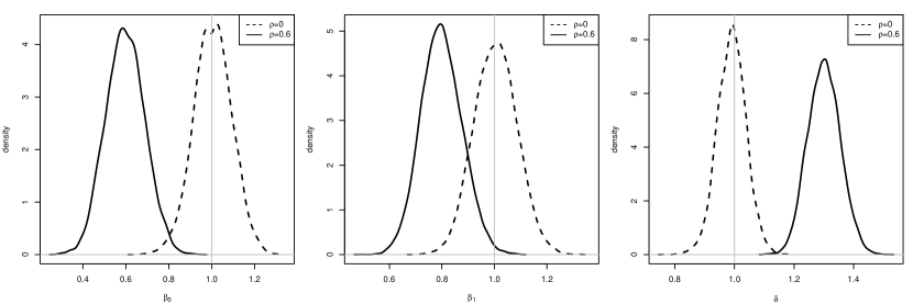
Figure 1: Posterior distributions of $\beta_{0}$, $\beta_{1}$, and $\delta$ using the standard Bayesian Tobit median regression

3 Bayesian Endogenous TQR Model

3.1 Model

We propose the following model to deal with the endogenous variables:

$$y_{i}^{*} = \mathbf{x}_{i}^{\prime}\text{\boldmath{$\beta$}}_{p}+\delta_{p}d_{i}+\eta_{p}(d_{i}-\mathbf{z}_{i}^{\prime}\text{\boldmath{$\gamma$}})+e_{i},$$ (5)

$$d_{i} = \mathbf{z}_{i}^{\prime}\text{\boldmath{$\gamma$}}+v_{i},$$ (6)

for $i=1,\dots,n$, where $\mathbf{x}_{i}$ is the vector of the exogenous variables whose the first element is $1$, $d_{i}$ is the endogenous variable, $\mathbf{z}_{i}=(\mathbf{x}_{i}^{\prime},w_{i})^{\prime}$, and $w_{i}$ is the exogenous variable not included in $\mathbf{x}_{i}$, which is also called the instrumental variable. The term $d_{i}-\mathbf{z}_{i}^{\prime}\text{\boldmath{$\gamma$}}=v_{i}$ in (5) is called the control variable and is introduced to account for endogeneity. Note that $\eta_{p}\neq 0$ indicates $d_{i}$ is endogenous. We refer to (6) as the first stage regression and to (5) as the second stage regression. A similar form is found in Lopes and Polson (2014) in the context of the instrumental variable regression for means by using the Cholesky-based prior.

Following Lee (2007), the error term $\epsilon_{i}$ of the standard Bayesian TQR is decomposed into the terms $\eta_{p}(d_{i}-\mathbf{z}_{i}^{\prime}\text{\boldmath{$\gamma$}})$ and $e_{i}$. It is assumed that relationship (6) is specified correctly and the quantile independence of $e_{i}$ on $\mathbf{z}_{i}$ conditional on $v_{i}$:

$$Q_{\epsilon|d,\mathbf{z}}(p)=Q_{\epsilon|v,\mathbf{z}}(p)=Q_{\epsilon|v}(p)=\eta_{p}(d-\mathbf{z}^{\prime}\text{\boldmath{$\gamma$}}).$$ (7)

As in Lee (2007), we also assume

$$Q_{v|\mathbf{z}}(\alpha)=0,$$ (8)

where the $\alpha$-th conditional quantile of $v_{i}$ is zero for some $\alpha\in(0,1)$.

3.2 First Stage Regression

We are mainly concerned with modelling the first stage error that satisfies (8). A simple and convenient approach is to assume $v_{i}\sim\mathcal{AL}(\phi,\alpha),\ i=1,\dots,n,$ as in Ogasawara and Kobayashi (2015), since (8) is always satisfied for the asymmetric Laplace distribution. However, the asymmetric Laplace distribution has limitations, such as peaky density, restrictive tail behaviour, and skewness. When a model lacks fit to the data, the estimate of the conditional quantile would be away from the value such that (8) truly holds. Then, assuming $v_{i}$ is homoskedastic, the estimate of the intercept, $\gamma_{0}$, may be biased as well. Consequently, the estimate of $\text{\boldmath{$\beta$}}_{p0}$ would be affected through the introduced term $\eta_{p}(d_{i}-\mathbf{z}_{i}^{\prime}\text{\boldmath{$\gamma$}})$. When $v_{i}$ is heteroskedastic, the entire coefficient vector would be affected. Therefore, we consider some alternative models for the first stage error distribution.

Recently, Wichitaksorn et al. (2014) considered a class of parametric distributions with a quantile constraint of the form (8), including the asymmetric Laplace distribution, and applied them in the context of quantile modelling. Furthermore, Zhu and Zinde-Walsh (2009), Zhu and Galbraith (2011), and Naranjo et al. (2015) considered a flexible parametric distribution with the quantile constraint. Based on these studies, we also consider the following two distributions to model the first stage error.

First, we consider the skew normal distribution denoted by $\mathcal{SN}(\phi,\alpha)$, where $\phi>0$ is the scale parameter and $\alpha\in(0,1)$ is the shape parameter. The probability density function is given by

$$f_{SN}(v|\phi,\alpha)=\frac{4\alpha(1-\alpha)}{\sqrt{2\pi\phi}}\exp\left\{-\frac{v^{2}}{2\phi}4(\alpha-I(v\leq 0))^{2}\right\}.$$ (9)

When $\alpha=0.5$, the distribution reduces to $\mathcal{N}(0,\phi)$. The mean and variance are given by $E[v]=\sqrt{\frac{\phi}{2\pi}}\frac{1-2\alpha}{\alpha(1-\alpha)}$ and $\text{Var}(v)=\phi\frac{\pi(1-3\alpha+3\alpha^{2})-2(1-2\alpha)^{2}}{4\pi\alpha^{2}(1-\alpha)^{2}}$ (see Wichitaksorn et al., 2014). When the actual error distribution is close to the normal distribution, this distribution would lead to better performance than the asymmetric Laplace distribution. However, just as the asymmetric Laplace distribution, the skewness and the quantile level of the mode are controlled by the single parameter $\alpha$.

Second, we consider the asymmetric exponential power distribution treated by Zhu and Zinde-Walsh (2009), Zhu and Galbraith (2011), and Naranjo et al. (2015). The probability density function of the asymmetric exponential power distribution, denoted by $\mathcal{AEP}(\phi,\alpha,\zeta_{1},\zeta_{2})$, is given by

$$f_{AEP}(v|\phi,\alpha,\zeta_{1},\zeta_{2})=\left\{\begin{array}[]{ll}\frac{1}{\phi}\exp\left\{-\left|\frac{v}{\alpha\phi/\Gamma(1+1/\zeta_{1})}\right|^{\zeta_{1}}\right\},&\text{if}\quad v\leq 0,\\ \frac{1}{\phi}\exp\left\{-\left|\frac{v}{(1-\alpha)\phi/\Gamma(1+1/\zeta_{2})}\right|^{\zeta_{2}}\right\},&\text{if}\quad v>0,\\ \end{array}\right.$$ (10)

where $\phi>0$ is the scale parameter, $\alpha\in(0,1)$ is the skewness parameter, $\zeta_{1}>0$ is the shape parameter for the left tail, and $\zeta_{2}>0$ is the shape parameter for the right tail. After some reparameterisation, the distribution reduces to the asymmetric Laplace distribution when $\zeta_{1}=\zeta_{2}=1$ and to the skew normal distribution when $\zeta_{1}=\zeta_{2}=2$. The tails of the asymmetric exponential power distribution are controlled separately by $\zeta_{1}$ and $\zeta_{2}$, respectively, and the overall skewness is controlled by $\alpha$. Although the distribution is more flexible than the above two distributions, the posterior computation using MCMC would be inefficient, because it includes two additional shape parameters and it has no convenient mixture representation, apart from the mixture of uniforms that is inefficient, to facilitate an efficient MCMC algorithm. The computational efficiency is also compared in Section 4.

In addition to the three parametric models, we also consider the semiparametric extension of the models based on the asymmetric Laplace and skew normal distributions to achieve both flexibility and computational efficiency. More specifically, the following two models using the Dirichlet process mixtures of scales are considered:

$$f_{ALDP}(v|G)=\int f_{AL}(v|\phi,\alpha)dG(\phi),\quad G\sim\mathcal{DP}(a,G_{0}),$$ (11)

$$f_{SNDP}(v|G)=\int f_{SN}(v|\phi,\alpha)dG(\phi),\quad G\sim\mathcal{DP}(a,G_{0}),$$ (12)

where $\mathcal{DP}(a,G_{0})$ denotes the Dirichlet process with the precision parameter $a>0$ and the base measure $G_{0}$. For both models, we set $G_{0}=\mathcal{IG}(c_{0},d_{0})$ as it is computationally convenient. While those mixture models have the same limitation as the parametric versions in terms of skewness, they extend the tail behaviour of the error distribution preserving (8) (Kottas and Krnjajić, 2009). Hereafter, the models with the asymmetric Laplace, skew normal, and asymmetric exponential power first stage errors are respectively denoted by AL, SN, and AEP, and those with the Dirichlet process mixtures are denoted by ALDP and SNDP.

We must take care when selecting the $\alpha$ value in (8), as it is a part of the model specification and can thus affect the estimates (Lee, 2007). We treat $\alpha$ as a parameter and estimate its value along with the other parameters. Since $\alpha$ determines the quantile level of the mode for all models considered here, our approach to modelling the first stage regression can also be regarded as a kind of mode regression (see Wichitaksorn et al., 2014).

To gain further flexibility, we might extend the model through a fully nonparametric mixture. Several semiparametric models in the context of Bayesian quantile regression with exogenous variables have been proposed by Kottas and Gelfand (2001), Kottas and Krnjajić (2009), and Reich et al. (2010). For example, Kottas and Krnjajić (2009) considered the nonparametric mixture of uniform distributions for any unimodal density on the real line with the quantile restriction at the mode using the Dirichlet process mixture (see also Kottas and Gelfand, 2001). In the more flexible model proposed by Reich et al. (2010), the mode of the error distribution does not have to coincide with zero. This is achieved by using a nonparametric mixture of the quantile-restricted two-component mixtures of normal distributions. However, their approaches are not directly applicable in the present context where the value of $\alpha$ is estimated. If we were to estimate the quantile level for which the quantile restriction holds, the computation under the former model is expected to be extremely inefficient and unstable as the model involves many indicator functions, and $\alpha$ and the intercept would be highly correlated. The intercept would not be identifiable in the latter model.

We could further extend the model to account for heteroskedasticity such that

$$d_{i}=\mathbf{z}_{i}^{\prime}\text{\boldmath{$\gamma$}}+\mathbf{z}_{i}^{\prime}\text{\boldmath{$\kappa$}}v_{i},$$ (13)

for $i=1,\dots,n$, where $\mathbf{z}_{i}^{\prime}\text{\boldmath{$\kappa$}}>0$ for all $i$ and the first element of $\kappa$ is fixed to one (e.g. Reich, 2010). In this case, the $\alpha$-th quantile of $d$ is given by $Q_{d|\mathbf{z}}(\alpha)=\mathbf{z}_{i}^{\prime}\text{\boldmath{$\gamma$}}+\mathbf{z}_{i}^{\prime}\text{\boldmath{$\kappa$}}Q_{v|\mathbf{z}}(\alpha)=\mathbf{z}_{i}^{\prime}(\text{\boldmath{$\gamma$}}+\text{\boldmath{$\kappa$}}Q_{v|\mathbf{z}}(\alpha))$ as in the usual quantile regression. However, since the first stage regression model is built based on (8), models (6) and (13) would produce identical estimates.

3.3 Second Stage Regression

We next turn to the model of the new second stage error, $e_{i}$, in (5). Since the $p$-th conditional quantile of $e_{i}$ is now zero, we assume that $e_{i}\sim\mathcal{AL}(\sigma,p),\ i=1,\dots,n,$ as in the standard Bayesian quantile regression approach. We utilise the location scale mixture of normals representation for the asymmetric Laplace distribution to facilitate an efficient MCMC method following Kozumi and Kobayashi (2011) (see also Kotz et al., 2001). The model is expressed in the hierarchical form given by

$$y_{i} = \max\left\{y_{i}^{*},0\right\},$$

$$y_{i}^{*} \sim \mathcal{N}(\tilde{\mathbf{x}}_{i}^{\prime}\tilde{\text{\boldmath{$\beta$}}}_{p}+\theta_{p}g_{i},\tau_{p}^{2}\sigma g_{i}),$$

$$g_{i} \sim \mathcal{E}(\sigma),$$

for $i=1,\dots,n$, where $\tilde{\mathbf{x}}_{i}=(\mathbf{x}_{i}^{\prime},d_{i},d_{i}-\mathbf{z}_{i}^{\prime}\text{\boldmath{$\gamma$}})^{\prime}$, $\tilde{\text{\boldmath{$\beta$}}}_{p}=(\text{\boldmath{$\beta$}}_{p}^{\prime},\delta_{p},\eta_{p})^{\prime}$, $\mathcal{E}(\sigma)$ denotes the exponential distribution with mean $\sigma$, and

$$\theta_{u}=\frac{1-2p}{p(1-p)},\quad\tau^{2}_{p}=\frac{2}{p(1-p)}.$$ (14)

3.4 Prior Distributions

The coefficient parameter $\gamma$ is common to all first stage regression specifications. First, we assume the normal prior for $\gamma$, since it is computationally convenient for the AL, SN, ALDP, and SNDP models. Since we do not have information on the coefficient values, the variances are set such that the prior distributions are relatively diffuse. Our default choice is $\text{\boldmath{$\gamma$}}\sim\mathcal{N}(\mathbf{0},100\mathbf{I})$. For the scale parameters, $\phi$ for the AL, SN, and AEP distributions, a relatively diffuse inverse gamma distribution is assumed and the default choice is set to $\mathcal{IG}(0.1,0.1)$. For AEP, we assume $\zeta_{j}\sim\mathcal{TN}_{(0,\infty)}(1,1)$, where $\mathcal{TN}_{(a,b)}(\mu,\sigma^{2})$ denotes the normal distribution with the mean $\mu$ and variance $\sigma^{2}$ truncated on the interval $(a,b)$. A similar prior specification is found in Naranjo et al. (2015). For all models, $\alpha\sim\mathcal{U}(0,1)$ is assumed.

For the semiparametric models, we need to specify the parameters of the inverse gamma base measure. Assuming that the data have been rescaled, $c_{0}$ and $d_{0}$ are chosen such that the variance of $v_{i}$ takes values between $0$ and $3$ with high probability (e.g. Ishwaran and James, 2002). Our default choice is $c_{0}=2$ and $d_{0}=0.5$ for ALDP and $c_{0}=d_{0}=1.5$ for SNDP. Under this choice, when $\alpha=0.5$ for ALDP, $\Pr(\phi_{l}\leq\sqrt{3.0/8})=0.802$ as $\text{Var}(v_{i})=8\phi^{2}$. Similarly, when $\alpha=0.4$, $\Pr(\phi_{l}\leq\sqrt{3.0/0.332})=0.784$. For SNDP, $\Pr(\phi_{l}\leq 3)=0.801$ when $\alpha=0.5$ and $\Pr(\phi_{l}\leq 3/1.104)=0.775$ when $\alpha=0.4$. For the precision parameter of the Dirichlet process, $a$, we assume $a\sim\mathcal{G}(2,2)$ such that both small and large values for $a$, hence the number of clusters, are allowed.

For the coefficient parameters in the second stage, $\text{\boldmath{$\beta$}}_{p}$ and $\delta_{p}$, we also assume relatively diffuse normal distributions. Our default choice of prior is $(\text{\boldmath{$\beta$}}_{p}^{\prime},\eta_{p})^{\prime}\sim\mathcal{N}(\mathbf{0},100\mathbf{I})$. Similar to $\phi$ in the parametric first stage, we assume an inverse gamma prior for the scale of the AL pseudo likelihood. Our default choice is $\mathcal{IG}(0.1,0.1)$.

The parameter $\eta_{p}$ accounts for the endogeneity and we need to take care in prior elicitation. When the data follow the bivariate normal distribution, as in the motivating example (3), $\eta_{p}$ is equal to $\rho\sigma_{1}/\sigma_{2}$, where $\rho$ is the correlation coefficient and $\sigma_{1}$ and $\sigma_{2}$ are the standard deviations of the first and second stage errors, respectively. In this case, we may follow Lopes and Polson (2014) to determine the variance of the normal prior implied from an inverse Wishart prior for the covariance matrix. However, we do not limit ourselves to normal data as the quantile regression approach is suitable for heteroskedastic and non-normal data, and the non-normal models are used in the first stage. In the literature on Bayesian non-normal selection models, the prior distribution of $\eta_{p}$ is normal typically with a very small variance, such as $1/2$ (e.g. Munkin and Trivedi, 2003, 2008; Deb et al., 2006). On the other hand, we use a more diffused prior to reflect our ignorance about $\eta_{p}$ and set our default choice of prior to be $\eta_{p}\sim\mathcal{N}(0,5)$. When the instrument is weak, it is expected that our quantile regression models face the problem of prior sensitivity and that the posterior distributions exhibit sharp behaviour, as in the case of the Bayesian instrumental variable regression model. Section 4 considers the alternative choices of the hyperparameters to study the prior sensitivity.

3.5 MCMC Method

The proposed models are estimated by using the MCMC method based on the Gibbs sampler. We describe the Gibbs sampler for the semiparametric models with ALDP and SNDP, which is an extension of the Gibbs sampler described in Kozumi and Kobayashi (2011) and Ogasawara and Kobayashi (2015). The algorithms for the AL and SN models can be obtained straightforwardly. We also mention the algorithm for the AEP model.

The variables involved in the Dirichlet process are sampled by using the retrospective sampler (Papaspiliopoulos and Roberts, 2008) and the slice sampler (Walker, 2007). First, we introduce $u_{i}\sim\mathcal{U}(0,1)$ and $k_{i},\ i=1,\dots,n$, such that $\pi_{l}=\Pr(k_{i}=l),l=1,\dots,\infty$. Then, as in Walker (2007), the Gibbs sampler is constructed by working on the following joint densities

$$f_{ALDP}(v_{i},u_{i})=\sum_{l=1}^{\infty}I(u_{i}<\omega_{l})f_{AL}(v_{i}|\phi_{l},\alpha),$$

$$f_{SNDP}(v_{i},u_{i})=\sum_{l=1}^{\infty}I(u_{i}<\omega_{l})f_{SN}(v_{i}|\phi_{l},\alpha),$$

where $\phi_{l}\sim G_{0}$, $\pi_{l}=\omega_{l}\prod_{l<r}(1-\omega_{r})$, $\omega_{l}\sim\mathcal{B}(1,a)$, and $\mathcal{B}(a,b)$ denotes the beta distribution with the parameters $a$ and $b$ (Sethuraman, 1994). We also let $k^{*}$ denote the minimum integer such that $\sum_{l=1}^{k^{*}}\pi_{l}>1-\min\left\{u_{1},\dots,u_{n}\right\}$.

Algorithm for ALDP

For the ALDP model, we utilise the mixture representation for the asymmetric Laplace distribution to sample $\gamma$ efficiently such that $v_{i}|h_{i}\sim\mathcal{N}(\theta_{\alpha}h_{i},\tau^{2}_{a}\phi_{i}h_{i})$, $h_{i}\sim\mathcal{E}(\phi_{i})$, $i=1,\dots,n$, where $\theta_{a}$ and $\tau^{2}_{a}$ are defined as in (14). Let us denote $\tilde{\text{\boldmath{$\beta$}}}_{p}=(\text{\boldmath{$\beta$}}_{p}^{\prime},\delta_{p},\eta_{p})^{\prime}$ and $\tilde{\mathbf{x}}_{i}=(\mathbf{x}_{i}^{\prime},d_{i},v_{i}-\mathbf{z}_{i}^{\prime}\text{\boldmath{$\gamma$}})^{\prime}$. Our Gibbs sampler proceeds by alternately sampling $\left\{u_{i}\right\}_{i=1}^{n}$, $\left\{\omega_{l}\right\}_{l=1}^{k^{*}}$, $\left\{k_{i}\right\}_{i=1}^{n}$, $\left\{\phi_{l}\right\}_{l=1}^{k^{*}}$, $a$, $\gamma$, $\left\{h_{i}\right\}_{i=1}^{n}$, $\alpha$, $\left\{y_{i}^{*}\right\}_{i=1}^{n}$, $\tilde{\text{\boldmath{$\beta$}}}_{p}$, $\sigma$, and $\left\{g_{i}\right\}_{i=1}^{n}$.

• Sampling $\left\{u_{i}\right\}_{i=1}^{n}$: Generate $u_{i}$ from $\mathcal{U}(0,\pi_{k_{i}})$ for $i=1,\dots,n$.

• Sampling $\left\{\omega_{l}\right\}_{l=1}^{k^{*}}$: Generate $\omega_{l}$ from $\mathcal{B}(1+n_{l},n-\sum_{r\leq l}n_{r}+a)$ where $n_{l}=\sum_{i=1}^{n}I(k_{i}=l)$ for $l=1,\dots,k^{*}$.

• Sampling $\left\{k_{i}\right\}_{i=1}^{n}$: Generate $k_{i}$ from the multinomial distribution with probabilities

  $$\Pr(k_{i}=l)\propto f_{AL}(d_{i}-\mathbf{z}_{i}^{\prime}\text{\boldmath{$\gamma$}}|\phi_{l},\alpha)I(u_{i}<\pi_{l}),\ l=1,\dots,k^{*}.$$

  for $i=1,\dots,n$.

• Sampling $\left\{\phi_{l}\right\}_{l=1}^{k^{*}}$: Generate $\phi_{l}$ from $\mathcal{IG}(c_{l},d_{l})$ where

  $$c_{l}=1.5n_{l}+c_{0},\quad d_{l}=\sum_{i:k_{i}=l}\left[h_{i}+\frac{(d_{i}-\mathbf{z}_{i}^{\prime}\text{\boldmath{$\gamma$}}-\theta_{\alpha}h_{i})^{2}}{2\tau_{\alpha}^{2}h_{i}}\right]+d_{0}.$$

• Sampling $a$: Assuming the gamma prior, $\mathcal{G}(a_{0},b_{0})$, we use the method described by Escobar and West (1995) to sample $a$. By introducing $c\sim\mathcal{B}(a+1,n)$, the full conditional distribution of $a$ is the mixture of two gamma distributions given by

  $$\varphi\mathcal{G}(a_{0}+n^{*},b_{0}-\log c)+(1-\varphi)\mathcal{G}(a_{0}+n^{*}-1,b_{0}-\log c),$$

  where $n^{*}$ is the number of distinct clusters and $\varphi/(1-\varphi)=(a_{0}+n^{*}-1)/(n(b_{0}-\log c))$.

• Sampling $\gamma$: Assuming $\text{\boldmath{$\gamma$}}\sim\mathcal{N}(\mathbf{g}_{0},\mathbf{G}_{0})$, $\gamma$ is sampled from $\mathcal{N}(\mathbf{g}_{1},\mathbf{G}_{1})$ where

  $$\mathbf{G}_{1} = \left[\sum_{i=1}^{n}\mathbf{z}_{i}\left(\frac{\eta_{p}^{2}}{\tau_{p}^{2}\sigma g_{i}}+\frac{1}{\tau^{2}_{\alpha}\phi_{k_{i}}h_{i}}\right)\mathbf{z}_{i}^{\prime}+\mathbf{G}_{0}^{-1}\right]^{-1},$$

  $$\mathbf{g}_{1} = \mathbf{G}_{1}\left[\sum_{i=1}^{n}\mathbf{z}_{i}\left(-\frac{\eta_{p}(y_{i}^{*}-\mathbf{x}_{i}^{\prime}\text{\boldmath{$\beta$}}_{p}-\eta_{p}d_{i}-\theta_{p}g_{i})}{\tau_{p}^{2}\sigma g_{i}}+\frac{d_{i}-\theta_{\alpha}h_{i}}{\tau_{\alpha}^{2}\phi_{k_{i}}h_{i}}\right)+\mathbf{G}_{0}^{-1}\mathbf{g}_{0}\right],$$

  as the density of the full conditional distribution denoted by $\pi(\text{\boldmath{$\gamma$}}|-)$ is given by

  $$\pi(\text{\boldmath{$\gamma$}}|-) \propto \exp\left\{-\sum_{i=1}^{n}\frac{(y_{i}^{*}-\mathbf{x}_{i}^{\prime}\text{\boldmath{$\beta$}}_{p}-\delta_{p}d_{i}-\eta_{p}(d_{i}-\mathbf{z}_{i}^{\prime}\text{\boldmath{$\gamma$}})-\theta_{p}g_{i})^{2}}{2\tau_{p}^{2}\sigma g_{i}}\right\}$$

  $$\times\exp\left\{-\sum_{i=1}^{n}\frac{(d_{i}-\mathbf{z}_{i}^{\prime}\text{\boldmath{$\gamma$}})^{2}}{2\tau_{\alpha}^{2}\phi_{k_{i}}h_{i}}\right\}\exp\left\{-\frac{1}{2}(\text{\boldmath{$\gamma$}}-\mathbf{g}_{0})^{\prime}\mathbf{G}_{0}^{-1}(\text{\boldmath{$\gamma$}}-\mathbf{g}_{0})\right\}$$

  $$\propto \exp\left\{-\frac{1}{2}(\text{\boldmath{$\gamma$}}-\mathbf{g}_{1})^{\prime}\mathbf{G}_{1}^{-1}(\text{\boldmath{$\gamma$}}-\mathbf{g}_{1})\right\}.$$

• Sampling $\left\{h_{i}\right\}_{i=1}^{n}$: The full conditional distribution of $h_{i}$ is the generalised inverse Gaussian distribution, denoted by $\mathcal{GIG}(\nu,\xi,\chi)$. The probability density function of $\mathcal{GIG}(\nu,\xi,\chi)$ is given by

  $$f(x|\nu,\xi,\chi)=\frac{(\chi/\xi)^{\nu}}{2K_{\nu}(\xi\chi)}x^{\nu-1}\exp\left\{-\frac{1}{2}(\xi^{2}x^{-1}+\chi^{2}x)\right\},\quad x>0,\quad-\infty<\nu<\infty,\quad\xi,\chi\geq 0,$$

  where $K_{\nu}(\cdot)$ is the modified Bessel function of the third kind (Barndorff-Nielsen and Shephard, 2001). For $i=1,\dots,n$, we sample $h_{i}$ from $\mathcal{GIG}(1/2,\xi_{i},\chi_{i})$ where

  $$\xi_{i}^{2}=\frac{(d_{i}-\mathbf{z}_{i}^{\prime}\text{\boldmath{$\gamma$}})^{2}}{\tau_{\alpha}^{2}\phi_{k_{i}}},\quad\chi^{2}_{i}=\frac{\theta_{a}^{2}}{\tau_{\alpha}^{2}\phi_{k_{i}}}+\frac{2}{\phi_{k_{i}}}.$$

• Sampling $\alpha$: The density of the full conditional distribution of $\alpha$ is given by

  $$\pi(\alpha|-)\propto\pi(\alpha)\prod_{i=1}^{n}f_{AL}(d_{i}-\mathbf{z}_{i}^{\prime}\text{\boldmath{$\gamma$}}|\phi_{k_{i}},\alpha),$$

  where $\pi(\alpha|-)$ and$\pi(\alpha)$ denote the full conditional and prior density of $\alpha$, respectively. We use the random walk Metropolis–Hastings (MH) algorithm to sample from this distribution.

• Sampling $\left\{y_{i}^{*}\right\}_{i=1}^{n}$: The full conditional distribution of $y_{i}^{*}$ is given by

  $$y_{i}I(y_{i}>0)+\mathcal{TN}_{(-\infty,0)}(\tilde{\mathbf{x}}_{i}^{\prime}\tilde{\text{\boldmath{$\beta$}}}_{p}+\theta_{p}g_{i},\tau_{p}^{2}\sigma g_{i})I(y_{i}=0),\quad i=1,\dots,n.$$

• Sampling $\tilde{\text{\boldmath{$\beta$}}}_{p}$: We sample $\tilde{\text{\boldmath{$\beta$}}}_{p}=(\text{\boldmath{$\beta$}}_{p}^{\prime},\delta_{p},\eta_{p})^{\prime}$ in one block. Assuming $\tilde{\text{\boldmath{$\beta$}}}_{p}\sim\mathcal{N}(\tilde{\mathbf{b}}_{0},\tilde{\mathbf{B}}_{0})$, the full conditional distribution is given by $\mathcal{N}(\tilde{\mathbf{b}}_{1},\tilde{\mathbf{B}}_{1})$ where

  $$\tilde{\mathbf{B}}_{1}=\left[\sum_{i=1}^{n}\frac{\tilde{\mathbf{x}}_{i}\tilde{\mathbf{x}}_{i}^{\prime}}{\tau_{p}^{2}\sigma g_{i}}+\tilde{\mathbf{B}}_{0}^{-1}\right]^{-1},\quad\tilde{\mathbf{b}}_{1}=\tilde{\mathbf{B}}_{1}\left[\sum_{i=1}^{n}\frac{\tilde{\mathbf{x}}_{i}(y_{i}^{*}-\theta_{p}g_{i})}{\tau_{p}^{2}\sigma g_{i}}+\tilde{\mathbf{B}}_{0}^{-1}\tilde{\mathbf{b}}_{0}\right].$$

• Sampling $\sigma$: Assuming $\sigma\sim\mathcal{IG}(m_{0},s_{0})$, we sample $\sigma$ from $\mathcal{IG}(m_{1},s_{1})$ where $m_{1}=1.5n+m_{0}$ and $s_{1}=\sum_{i=1}^{n}g_{i}+\sum_{i=1}^{n}(y_{i}-\tilde{\mathbf{x}}_{i}^{\prime}\tilde{\text{\boldmath{$\beta$}}}_{p}-\theta_{p}g_{i})^{2}/2\tau_{p}^{2}g_{i}+s_{0}$.

• Sampling $\left\{g_{i}\right\}_{i=1}^{n}$: Similar to $h_{i}$, $g_{i}$ is sampled from $\mathcal{GIG}(1/2,\lambda_{i},\psi)$ where

  $$\lambda_{i}^{2}=\frac{(y_{i}^{*}-\tilde{\mathbf{x}}_{i}^{\prime}\tilde{\text{\boldmath{$\beta$}}}_{p})^{2}}{\tau_{p}^{2}\sigma},\quad\psi^{2}=\frac{\theta_{p}^{2}}{\tau_{p}^{2}\sigma}+\frac{2}{\sigma},\quad i=1,\dots,n.$$

Algorithm for SNDP

The Gibbs sampler for SNDP consists of sampling $\left\{u_{i}\right\}_{i=1}^{n}$, $\left\{\omega_{l}\right\}_{l=1}^{k^{*}}$, $\left\{k_{i}\right\}_{i=1}^{n}$, $\left\{\phi_{l}\right\}_{l=1}^{k^{*}}$, $a$, $\gamma$, $\alpha$, $\left\{y_{i}^{*}\right\}_{i=1}^{n}$, $\tilde{\text{\boldmath{$\beta$}}}_{p}$, $\sigma$, and $\left\{g_{i}\right\}_{i=1}^{n}$. The sampling algorithms for $\left\{u_{i}\right\}_{i=1}^{n}$, $\left\{\omega_{l}\right\}_{l=1}^{k^{*}}$, $a$, $\left\{y_{i}^{*}\right\}_{i=1}^{n}$, $\tilde{\text{\boldmath{$\beta$}}}_{p}$, $\sigma$, and $\left\{g_{i}\right\}_{i=1}^{n}$ remain the same as in the case of ALDP. The sampling scheme of $\left\{k_{i}\right\}_{i=1}^{n}$ and $\alpha$ can be obtained by replacing $f_{AL}(d_{i}-\mathbf{z}_{i}^{\prime}\text{\boldmath{$\gamma$}}|\phi_{k_{i}},\alpha)$ with $f_{SN}(d_{i}-\mathbf{z}_{i}^{\prime}\text{\boldmath{$\gamma$}}|\phi_{k_{i}},\alpha)$.

Similar to the case of ALDP, the density of the full conditional distribution is given by

$$\pi(\text{\boldmath{$\gamma$}}|-)\propto\exp\left\{-\frac{1}{2}(\text{\boldmath{$\gamma$}}-\mathbf{g}_{1}(\text{\boldmath{$\gamma$}}))^{\prime}\mathbf{G}_{1}(\text{\boldmath{$\gamma$}})^{-1}(\text{\boldmath{$\gamma$}}-\mathbf{g}_{1}(\text{\boldmath{$\gamma$}}))\right\},$$

where

$$\mathbf{G}_{1}(\text{\boldmath{$\gamma$}}) = \left[\sum_{i=1}^{n}\mathbf{z}_{i}\left(\frac{\eta_{p}^{2}}{\tau_{p}^{2}\sigma g_{i}}+\frac{4(\alpha-I(d_{i}\leq\mathbf{z}_{i}^{\prime}\text{\boldmath{$\gamma$}}))^{2}}{\phi_{k_{i}}}\right)\mathbf{z}_{i}^{\prime}+\mathbf{G}_{0}^{-1}\right]^{-1},$$

$$\mathbf{g}_{1}(\text{\boldmath{$\gamma$}}) = \mathbf{G}_{1}(\text{\boldmath{$\gamma$}})\left[\sum_{i=1}^{n}\mathbf{z}_{i}\left(-\frac{\eta_{p}(y_{i}^{*}-\mathbf{x}_{i}^{\prime}\text{\boldmath{$\beta$}}_{p}-\eta_{p}d_{i}-\theta_{p}g_{i})}{\tau_{p}^{2}\sigma g_{i}}+\frac{4d_{i}(\alpha-I(d_{i}\leq\mathbf{z}_{i}^{\prime}\text{\boldmath{$\gamma$}}))^{2}}{\phi_{k_{i}}}\right)+\mathbf{G}_{0}^{-1}\mathbf{g}_{0}\right],$$

which is similar to the density of the normal distribution. Therefore, we sample $\gamma$ by using the MH algorithm with the proposal distribution given by $\mathcal{N}(\mathbf{g}_{1}(\text{\boldmath{$\gamma$}}),\mathbf{G}_{1}(\text{\boldmath{$\gamma$}}))$.

Algorithm for AEP

Since no convenient representation for the AEP distribution is available, the full conditional distributions of the parameters in the first stage regression, $\gamma$, $\phi$, $\alpha$, $\zeta_{1}$, and $\zeta_{2}$, are not in the standard forms. Therefore, we employ the adaptive random walk MH algorithm. Although Naranjo et al. (2015) proposed the scale mixture of uniform representation for the AEP distribution, the algorithm based on this representation would be inefficient, because it consists of sampling from a series of distributions that are truncated on some intervals such that the mixture representation holds and such intervals move quite slowly as sampling proceeds (see also Kobayashi, 2015). Since the additional shape parameters in AEP free up the role of $\alpha$, $\alpha$ controls the overall skewness by allocating the weights on the left and right sides of the mode. Hence, the MCMC sample would exhibit relatively high correlation between $\alpha$ and $\gamma_{0}$.

4 Simulation Study

The models considered in the previous section are demonstrated using simulated data. The aims of this section are (1) to compare the performance of the proposed models (Section 4.2), (2) to study the sensitivity to the prior settings, and (3) to illustrate the behaviour of the posterior distribution when the instrument is weak (Section 4.3).

4.1 Settings

The data are generated from the model given by

$$\begin{split}y_{i}^{*}&=\beta_{0}+\beta_{1}x_{i}+\delta d_{i}+\eta v_{i}+e_{i},\\ d_{i}&=\gamma_{0}+\gamma_{1}x_{i}+\gamma_{2}w_{i}+v_{i},\end{split}$$ (15)

for $i=1,\dots,300$, where $(\gamma_{0},\gamma_{1},\gamma_{2})=(0,1,1.5)$ assuming that a valid instrument is available, $(\beta_{0},\beta_{1},\delta,\eta)=(0,1,1,0.6)$, $x_{i}\sim\mathcal{N}(0,1)$, and $w_{i}\sim\mathcal{TN}_{(0,\infty)}(1,1)$. The performance of the models is compared by considering the various settings for $v_{i}$, while the distributions of $e_{i}$ are kept relatively simple in order that the true values of the quantile regression coefficients are tractable. The following five settings are considered:
Setting 1 $v_{i}\sim\mathcal{N}(0,1)$, $e_{i}\sim\mathcal{N}(0,1-\eta^{2})$,
Setting 2 $v_{i}\sim t_{4}$, $e_{i}\sim t_{6}$,
Setting 3 $v_{i}\sim\mathcal{ST}(-0.430,1,0.980,4)$, $e_{i}\sim t_{6}$,
Setting 4 $v_{i}\sim\mathcal{N}(0,(1+0.5w_{i})^{2})$, $e_{i}\sim\mathcal{N}(0,1-\eta^{2})$,
Setting 5 $v_{i}\sim\mathcal{ST}(-0.430,(1+0.5w_{i})^{2},0.980,4)$, $e_{i}\sim t_{6}$,
where $\mathcal{ST}(\mu,\sigma^{2},\alpha,\nu)$ denotes the skew $t$ distribution with the location parameter $\mu$, scale parameter $\sigma^{2}$, skewness parameter $\alpha=\delta/\sqrt{1-\delta^{2}}$, $\delta\in(-1,1)$, and degree of freedom $\nu$ (see Azzalini and Capitanio, 2003; Fr$\ddot{\text{u}}$hwirth-Schnatter and Pyne, 2010), and we set $\delta=0.7$. In Setting 1, the error terms follow the bivariate normal distribution as in the motivating example in Section 2. Setting 2 considers the fat tailed first stage regression. Setting 3 considers a more difficult situation where the first stage error is fat tailed and skewed. Setting 4 replaces the first stage error of Setting 1 with the heteroskedastic error with respect to the instrument. Setting 5 is also a challenging situation where the first stage error is fat tailed, skewed, and heteroskedastic. In Settings 3 and 5, the location parameters of the first stage error distributions are set such that the mode of $v_{i}$ is zero and the quantile level of the mode is $0.435$. The average censoring rates for the settings are around $0.25$. For each setting, the data are replicated $100$ times.

4.2 Results under the Default Priors

We first estimated the proposed models under the default prior specifications (see Section 3.4) for $p=0.1$ and $0.5$ by running the MCMC for $20000$ iterations and discarding the first $5000$ draws as the burn-in period. The standard Bayesian TQR model was also estimated. The bias and root mean squared error (RMSE) of the parameters were computed over the $100$ replications. To assess the efficiency of the MCMC algorithm, we also recorded the inefficiency factor, which was defined as a ratio of the numerical variance of the sample mean of the Markov chain to the variance of the independence draws (Chib, 2001).

Table 1 presents the biases, RMSEs, and median inefficiency factors for the parameters over the $100$ replications. First, we examined the inefficiency factors. Overall, our sampling algorithms appear to be efficient, especially for AL, SN, ALDP, and SNDP. The table shows that the inefficiency factors for AL, SN, ALDP, and SNDP are reasonably small for $\beta_{p1}$, $\delta_{p}$, $\eta_{p}$, $\gamma_{1}$, and $\gamma_{2}$. Since $\alpha$ and $\gamma_{0}$ determine the quantile level of the mode and location of the mode, respectively, the MCMC sample exhibits correlation between $\alpha$ and $\gamma_{0}$ and this results in higher inefficiency factors for them. Hence, the inefficiency factors for $\beta_{p0}$ tend to be higher than those for the other parameters. This pattern is more profound in the case of AEP where the inefficiency factors for $\alpha$, $\gamma_{0}$, and $\beta_{p0}$ are quite high. Since the additional shape parameters in AEP free up the role of $\alpha$, the MCMC sample exhibits higher correlation between $\alpha$ and $\gamma_{0}$. Furthermore, the inefficiency factors for the other parameters for AEP are also higher than those for the other endogenous models.

Next, we turn to the performance of the models. As expected, TQR produces biased estimates in all cases. The RMSEs for the proposed endogenous models are generally larger for $p=0.1$, which is below the censoring point, than for $p=0.5$. The AL and ALDP models result in similar performance. The AEP model shows the largest RMSEs for $\gamma_{0}$ and $\beta_{p0}$ among the proposed models for all cases. Combined with the high inefficiency factors for those parameters, the convergence of the MCMC algorithm for AEP may be difficult to ensure in the given simulation setting. This finding suggests a considerable practical limitation and, thus, AEP will not be considered henceforth. The same limitation applies to the potentially more flexible nonparametric models discussed in Section 3.2.

Table 1 also shows that the estimation of the first stage regression can influence the second stage parameters. For example, in Setting 1, the RMSEs for $\gamma_{0}$ for SN and SNDP are smaller than those for AL and ALDP, as the true model is the normal and thus SN and SNDP produce smaller RMSEs for $\beta_{p0}$. Similarly, in Setting 4, the RMSEs for $\beta_{p0}$ for SN and SNDP are smaller than those for AL and ALDP. In addition, the heteroskedasticity in the first stage influences the performance of the slope parameters, resulting in slightly smaller RMSEs for $\beta_{p1}$ for SN and SNDP than for AL and ALDP. However, the performance of the SN model becomes worse when the first stage error is fat tailed, since the skew normal distribution cannot accommodate a fat tailed distribution. While the results in Setting 2 are somewhat comparable across the models, the table shows that SN results in larger biases and RMSEs in Setting 3 and, especially, Setting 5. In Setting 3, SN results in larger RMSEs for $\beta_{p0}$ than for AL, ALDP, and SNDP. In Setting 5, given the heteroskedasticity of the first stage, the biases and RMSEs for the intercept and slope parameters for SN are larger than those for AL, ALDP, and SNDP. On the other hand, compared with SN, the semiparametric SNDP model is able to cope with fat tailed errors and this produces results comparable with those for AL and ALDP.

While the models result in reasonable overall performance, the results for Settings 3 and 5 also illustrate the limitation of our modelling approach to some extent. In Setting 3, the models exhibit some bias in $\beta_{p0}$ because of the lack of fit in the first stage. This lack of fit, which is represented by the bias for $\gamma_{0}$, is reflected in the bias for $\beta_{p0}$. The entire coefficient vector may be influenced by this lack of fit in the first stage in the presence of heteroskedasticity as in Setting 5. The lack of fit in the first stage is also indicated by the biases in $\alpha$. This finding implies that an inflexible first stage model can fail to estimate the true quantile such that (8) holds and that choosing the value of $\alpha$ a priori could lead to biased estimates (see the discussion in Section 3.2).

Table 1: Biases, RMSEs, and inefficiency factors under the default priors

			TQR			AL			SN			AEP			ALDP			SNDP
Setting	$p$	Parameter	Bias	RMSE	IF	Bias	RMSE	IF	Bias	RMSE	IF	Bias	RMSE	IF	Bias	RMSE	IF	Bias	RMSE	IF
1	0.1	$\beta_{p0}$	-0.474	0.511	37.1	0.048	0.239	55.5	0.047	0.211	59.7	0.066	0.252	245.0	0.047	0.237	57.1	0.047	0.209	61.8
		$\beta_{p1}$	-0.248	0.272	17.0	-0.022	0.139	22.3	-0.020	0.134	18.9	-0.020	0.136	43.1	-0.022	0.140	24.7	-0.020	0.135	20.1
		$\delta_{p}$	0.200	0.212	27.4	-0.009	0.092	24.9	-0.007	0.085	20.0	-0.007	0.085	46.3	-0.008	0.092	24.6	-0.007	0.085	21.1
		$\eta_{p}$				0.001	0.122	18.5	-0.001	0.120	14.5	-0.001	0.120	29.8	0.000	0.122	17.5	-0.001	0.120	16.1
		$\gamma_{0}$				0.001	0.204	54.7	0.000	0.165	59.2	0.036	0.264	340.8	0.000	0.206	53.2	0.003	0.160	60.7
		$\gamma_{1}$				-0.012	0.066	16.7	-0.006	0.058	9.2	-0.007	0.060	96.3	-0.012	0.067	17.7	-0.007	0.059	9.6
		$\gamma_{2}$				-0.004	0.086	17.3	-0.002	0.074	9.2	-0.002	0.075	93.7	-0.004	0.086	16.9	-0.003	0.074	8.9
		$\alpha$				-0.002	0.052	66.1	-0.001	0.043	72.2	0.011	0.089	357.1	-0.002	0.054	65.0	-0.000	0.042	76.4
	0.5	$\beta_{p0}$	-0.426	0.443	11.7	0.017	0.180	25.5	0.018	0.167	34.6	0.030	0.196	243.7	0.017	0.182	25.3	0.017	0.165	34.1
		$\beta_{p1}$	-0.235	0.251	7.9	-0.001	0.089	12.8	0.001	0.087	9.9	0.001	0.088	27.3	-0.001	0.089	12.1	0.001	0.086	9.3
		$\delta_{p}$	0.233	0.238	9.7	-0.004	0.063	11.6	-0.003	0.061	10.1	-0.003	0.062	28.7	-0.004	0.063	11.6	-0.003	0.061	9.2
		$\eta_{p}$				0.004	0.086	8.7	0.003	0.084	8.2	0.003	0.085	18.3	0.004	0.086	8.2	0.003	0.083	7.6
		$\gamma_{0}$				0.003	0.206	37.6	0.003	0.163	44.2	0.028	0.254	313.0	0.003	0.209	41.0	0.003	0.161	47.4
		$\gamma_{1}$				-0.012	0.066	13.1	-0.006	0.058	5.7	-0.008	0.060	74.6	-0.012	0.066	12.2	-0.007	0.059	5.8
		$\gamma_{2}$				-0.005	0.085	12.0	-0.003	0.074	5.2	-0.003	0.075	60.5	-0.005	0.086	13.5	-0.003	0.074	5.9
		$\alpha$				-0.001	0.053	53.7	-0.000	0.043	57.1	0.008	0.086	328.5	-0.001	0.055	50.4	-0.000	0.042	62.3
2	0.1	$\beta_{p0}$	-0.594	0.657	53.6	0.088	0.302	40.5	0.082	0.309	50.2	0.099	0.354	120.4	0.090	0.304	40.6	0.096	0.305	47.6
		$\beta_{p1}$	-0.297	0.341	18.7	-0.009	0.161	22.3	-0.009	0.164	21.6	-0.008	0.159	38.0	-0.008	0.160	20.0	-0.010	0.160	21.1
		$\delta_{p}$	0.268	0.282	38.7	-0.025	0.115	23.4	-0.023	0.115	25.9	-0.024	0.115	35.9	-0.024	0.115	24.6	-0.023	0.115	24.1
		$\eta_{p}$				0.005	0.139	19.0	0.003	0.138	18.9	0.005	0.138	27.2	0.005	0.138	19.7	0.004	0.137	19.8
		$\gamma_{0}$				-0.025	0.189	27.8	-0.038	0.244	25.8	-0.001	0.339	203.2	-0.022	0.191	25.7	-0.015	0.176	32.6
		$\gamma_{1}$				0.001	0.073	11.6	0.003	0.082	7.8	0.000	0.070	70.1	0.001	0.073	12.4	-0.001	0.070	8.4
		$\gamma_{2}$				-0.002	0.092	12.1	0.004	0.094	8.2	-0.001	0.089	61.2	-0.002	0.092	14.6	0.002	0.087	8.1
		$\alpha$				-0.004	0.041	32.3	-0.005	0.059	32.3	0.004	0.107	212.1	-0.003	0.041	34.2	-0.000	0.036	46.2
	0.5	$\beta_{p0}$	-0.579	0.604	13.7	-0.001	0.198	16.6	-0.013	0.207	17.1	0.013	0.288	98.1	-0.000	0.200	17.4	0.004	0.193	18.9
		$\beta_{p1}$	-0.302	0.323	6.9	0.003	0.127	9.4	0.002	0.130	9.2	0.001	0.123	22.2	0.002	0.126	9.8	-0.001	0.123	8.1
		$\delta_{p}$	0.312	0.319	11.3	-0.004	0.082	9.0	-0.001	0.083	8.6	-0.002	0.080	20.3	-0.003	0.082	9.7	-0.001	0.080	8.4
		$\eta_{p}$				0.009	0.099	8.1	0.007	0.099	7.5	0.008	0.097	14.6	0.009	0.099	8.2	0.007	0.097	7.3
		$\gamma_{0}$				-0.025	0.188	20.8	-0.041	0.245	17.8	-0.003	0.341	165.9	-0.023	0.191	25.3	-0.015	0.176	24.0
		$\gamma_{1}$				0.001	0.073	9.2	0.003	0.082	5.0	0.000	0.070	58.6	0.001	0.073	10.7	-0.001	0.070	5.8
		$\gamma_{2}$				-0.002	0.091	9.3	0.005	0.094	4.7	0.001	0.089	50.2	-0.002	0.092	10.4	0.002	0.087	5.3
		$\alpha$				-0.004	0.041	29.7	-0.005	0.059	26.4	0.004	0.108	193.7	-0.003	0.041	35.8	-0.000	0.036	40.7
3	0.1	$\beta_{p0}$	-0.464	0.539	36.0	0.028	0.287	33.0	-0.006	0.301	36.4	0.113	0.334	108.2	0.027	0.288	35.4	0.026	0.282	37.7
		$\beta_{p1}$	-0.264	0.314	18.9	-0.007	0.180	18.1	-0.007	0.182	18.7	-0.010	0.181	31.5	-0.008	0.180	19.2	-0.009	0.182	17.8
		$\delta_{p}$	0.235	0.253	26.8	-0.022	0.120	17.4	-0.022	0.118	18.0	-0.021	0.118	27.9	-0.021	0.120	20.1	-0.021	0.118	18.7
		$\eta_{p}$				-0.011	0.149	14.5	-0.010	0.147	15.0	-0.012	0.148	21.7	-0.012	0.149	16.4	-0.011	0.147	12.8
		$\gamma_{0}$				-0.096	0.201	23.6	-0.147	0.285	23.9	0.041	0.309	199.4	-0.099	0.207	25.5	-0.098	0.186	27.7
		$\gamma_{1}$				0.001	0.058	10.9	1.001	1.003	6.4	-0.001	0.055	66.7	0.000	0.058	10.9	-0.001	0.057	5.4
		$\gamma_{2}$				-0.002	0.084	9.8	1.496	1.499	5.2	-0.001	0.079	60.1	-0.002	0.086	11.0	-0.002	0.077	6.1
		$\alpha$				-0.041	0.060	33.4	-0.055	0.089	35.1	0.020	0.116	214.8	-0.042	0.061	35.5	-0.039	0.055	48.0
	0.5	$\beta_{p0}$	-0.491	0.520	10.0	-0.053	0.191	13.6	-0.084	0.223	13.9	0.027	0.255	85.8	-0.054	0.192	14.5	-0.054	0.183	17.3
		$\beta_{p1}$	-0.268	0.288	6.7	0.014	0.117	8.6	0.015	0.123	7.3	0.011	0.117	18.7	0.013	0.117	9.3	0.012	0.120	6.6
		$\delta_{p}$	0.292	0.298	7.7	-0.006	0.072	9.2	-0.007	0.071	7.2	-0.006	0.073	16.4	-0.006	0.072	8.6	-0.007	0.072	7.5
		$\eta_{p}$				0.009	0.101	7.3	0.010	0.100	6.2	0.009	0.101	11.9	0.009	0.101	6.9	0.009	0.101	5.9
		$\gamma_{0}$				-0.096	0.202	19.1	-0.144	0.284	15.7	0.033	0.315	174.7	-0.098	0.206	24.6	-0.098	0.185	24.8
		$\gamma_{1}$				0.001	0.058	8.2	1.001	1.003	3.6	-0.002	0.055	51.5	0.001	0.058	9.9	-0.001	0.057	4.6
		$\gamma_{2}$				-0.002	0.084	8.7	1.496	1.499	3.9	-0.001	0.078	47.4	-0.002	0.086	9.1	-0.002	0.077	5.0
		$\alpha$				-0.040	0.060	27.7	-0.055	0.089	26.7	0.017	0.118	180.6	-0.041	0.060	34.9	-0.039	0.055	44.5
4	0.1	$\beta_{p0}$	-0.888	0.908	50.5	0.054	0.246	61.1	0.064	0.232	91.1	0.058	0.325	440.6	0.054	0.246	64.5	0.062	0.239	88.6
		$\beta_{p1}$	-0.401	0.416	20.1	0.001	0.148	49.7	0.006	0.143	53.1	0.007	0.144	114.2	0.002	0.153	42.7	0.005	0.144	52.9
		$\delta_{p}$	0.369	0.374	35.8	-0.018	0.101	49.0	-0.019	0.101	49.0	-0.019	0.099	128.8	-0.018	0.102	44.8	-0.017	0.098	56.2
		$\eta_{p}$				0.017	0.117	47.2	0.018	0.116	52.0	0.018	0.114	113.2	0.016	0.117	46.7	0.016	0.113	54.3
		$\gamma_{0}$				-0.005	0.249	59.0	0.010	0.217	97.9	-0.008	0.412	528.2	-0.005	0.248	58.2	0.009	0.227	92.4
		$\gamma_{1}$				-0.005	0.105	32.5	-0.001	0.096	27.1	-0.000	0.096	146.3	-0.005	0.106	31.5	-0.001	0.093	26.3
		$\gamma_{2}$				0.016	0.188	52.3	0.009	0.167	55.1	0.012	0.170	181.4	0.017	0.191	51.5	0.014	0.169	56.7
		$\alpha$				0.001	0.060	104.4	0.003	0.048	166.2	-0.001	0.090	549.6	0.002	0.061	113.3	0.004	0.053	148.9
	0.5	$\beta_{p0}$	-0.676	0.685	15.1	0.005	0.201	31.2	0.018	0.190	48.6	0.016	0.296	355.5	0.005	0.203	33.9	0.014	0.189	44.8
		$\beta_{p1}$	-0.388	0.397	7.7	-0.003	0.141	25.7	-0.001	0.129	24.2	-0.002	0.130	70.0	-0.002	0.144	23.7	-0.003	0.129	26.4
		$\delta_{p}$	0.380	0.382	11.7	-0.009	0.096	29.7	-0.010	0.088	28.4	-0.008	0.084	75.9	-0.010	0.098	28.6	-0.008	0.085	33.0
		$\eta_{p}$				0.023	0.106	26.5	0.024	0.098	27.0	0.022	0.095	65.9	0.024	0.108	25.8	0.022	0.095	29.8
		$\gamma_{0}$				-0.005	0.248	34.3	0.015	0.220	58.4	0.008	0.429	406.3	-0.004	0.251	37.7	0.011	0.220	57.0
		$\gamma_{1}$				-0.005	0.105	20.0	-0.001	0.095	14.1	-0.001	0.095	96.3	-0.004	0.105	23.2	-0.001	0.093	15.8
		$\gamma_{2}$				0.017	0.188	36.3	0.011	0.164	32.6	0.015	0.166	114.9	0.017	0.192	32.7	0.015	0.167	39.3
		$\alpha$				0.001	0.059	76.6	0.004	0.048	99.8	0.003	0.094	444.4	0.002	0.062	76.5	0.004	0.051	103.7
5	0.1	$\beta_{p0}$	-0.853	0.900	41.8	0.016	0.299	38.2	-0.032	0.339	47.6	0.155	0.408	158.2	0.014	0.298	39.0	-0.004	0.295	39.1
		$\beta_{p1}$	-0.405	0.438	20.9	0.028	0.198	27.1	0.045	0.222	33.3	0.029	0.202	58.1	0.030	0.198	25.1	0.030	0.205	25.9
		$\delta_{p}$	0.393	0.401	30.3	-0.048	0.146	26.6	-0.066	0.161	28.5	-0.049	0.145	61.1	-0.050	0.146	27.7	-0.051	0.148	26.4
		$\eta_{p}$				0.028	0.158	26.7	0.046	0.170	27.3	0.029	0.157	55.4	0.029	0.158	25.8	0.031	0.159	25.1
		$\gamma_{0}$				-0.093	0.240	26.8	-0.159	0.360	34.5	0.124	0.412	257.2	-0.097	0.247	25.5	-0.120	0.243	31.1
		$\gamma_{1}$				0.001	0.088	17.1	-0.000	0.127	16.7	0.001	0.087	74.4	0.001	0.088	16.8	-0.001	0.090	11.9
		$\gamma_{2}$				-0.056	0.160	24.9	-0.081	0.202	22.4	-0.055	0.156	104.9	-0.058	0.164	25.5	-0.064	0.161	20.6
		$\alpha$				-0.041	0.061	51.3	-0.057	0.094	57.3	0.020	0.101	288.7	-0.043	0.063	49.8	-0.048	0.066	65.7
	0.5	$\beta_{p0}$	-0.754	0.768	9.8	-0.042	0.201	16.0	-0.088	0.257	21.8	0.093	0.333	123.5	-0.043	0.206	17.3	-0.061	0.200	21.5
		$\beta_{p1}$	-0.394	0.406	7.0	0.052	0.148	15.2	0.068	0.181	13.9	0.049	0.147	35.1	0.052	0.148	14.4	0.052	0.154	12.1
		$\delta_{p}$	0.430	0.432	7.6	-0.042	0.102	15.1	-0.059	0.124	15.0	-0.040	0.100	41.7	-0.042	0.101	16.2	-0.045	0.105	14.0
		$\eta_{p}$				0.042	0.115	13.5	0.059	0.134	15.2	0.040	0.112	33.1	0.042	0.115	15.3	0.045	0.117	13.2
		$\gamma_{0}$				-0.093	0.239	18.7	-0.158	0.361	19.9	0.113	0.420	177.0	-0.095	0.247	21.4	-0.122	0.243	26.9
		$\gamma_{1}$				0.002	0.088	12.6	-0.000	0.127	9.5	0.000	0.086	59.9	0.001	0.088	14.4	-0.002	0.090	8.8
		$\gamma_{2}$				-0.058	0.162	19.3	-0.081	0.203	14.7	-0.052	0.155	75.0	-0.058	0.163	21.9	-0.064	0.161	16.3
		$\alpha$				-0.042	0.062	38.0	-0.057	0.094	42.0	0.018	0.104	209.2	-0.043	0.063	44.4	-0.049	0.067	54.2

4.3 Alternative Base Measures and Prior Specifications

For comparison purposes, we consider two alternative specifications for the inverse gamma base measure for the semiparametric models. The following slightly less diffuse settings than the default are considered. For ALDP, we consider $\mathcal{IG}(2.5,0.6)$ such that $\Pr(\phi_{l}\leq\sqrt{3/8})=0.854$ and $\mathcal{IG}(3.0,0.7)$ such that $\Pr(\phi_{l}\leq\sqrt{3/8})=0.891$ when $\alpha=0.5$. For SNDP, we consider $\mathcal{IG}(2,2)$ such that $\Pr(\phi\leq 3)=0.852$ and $\mathcal{IG}(2.5,2.5)$ such that $\Pr(\phi_{l}\leq 3)=0.893$. For the other parameters, we use the default prior specifications. Table 2 presents the biases and RMSEs for ALDP and SNDP under the alternative base measures for $p=0.1$ and $p=0.5$. The results in Table 2 are essentially identical to those in Table 1, suggesting that the default choice of the base measures provides reasonable performance.

Table 2: Biases and RMSEs for ALDP and SNDP under the alternative base measures

			ALDP				SNDP
			Alternative 1		Alternative 2		Alternative 1		Alternative 2
Setting	$p$	Parameter	Bias	RMSE	Bias	RMSE	Bias	RMSE	Bias	RMSE
1	0.1	$\beta_{p0}$	0.050	0.239	0.048	0.239	0.050	0.211	0.047	0.209
		$\beta_{p1}$	-0.022	0.140	-0.022	0.139	-0.020	0.136	-0.020	0.135
		$\delta_{p}$	-0.008	0.092	-0.009	0.092	-0.008	0.085	-0.007	0.086
	0.5	$\beta_{p0}$	0.018	0.182	0.017	0.183	0.017	0.164	0.019	0.164
		$\beta_{p1}$	-0.002	0.089	-0.001	0.089	0.001	0.087	0.001	0.087
		$\delta_{p}$	-0.004	0.063	-0.004	0.063	-0.003	0.061	-0.003	0.061
2	0.1	$\beta_{p0}$	0.092	0.304	0.088	0.304	0.091	0.302	0.094	0.302
		$\beta_{p1}$	-0.008	0.160	-0.007	0.160	-0.011	0.159	-0.012	0.158
		$\delta_{p}$	-0.025	0.115	-0.025	0.116	-0.022	0.114	-0.023	0.114
	0.5	$\beta_{p0}$	-0.001	0.199	-0.001	0.200	0.003	0.194	0.002	0.194
		$\beta_{p1}$	0.003	0.127	0.003	0.126	0.000	0.124	-0.001	0.123
		$\delta_{p}$	-0.003	0.082	-0.004	0.082	-0.002	0.081	-0.001	0.081
3	0.1	$\beta_{p0}$	0.025	0.286	0.025	0.287	0.024	0.280	0.022	0.282
		$\beta_{p1}$	-0.008	0.179	-0.009	0.180	-0.010	0.182	-0.010	0.182
		$\delta_{p}$	-0.020	0.119	-0.021	0.120	-0.021	0.118	-0.021	0.118
	0.5	$\beta_{p0}$	-0.056	0.193	-0.056	0.192	-0.056	0.183	-0.056	0.184
		$\beta_{p1}$	0.013	0.117	0.012	0.117	0.012	0.120	0.011	0.119
		$\delta_{p}$	-0.006	0.072	-0.006	0.072	-0.006	0.072	-0.006	0.072
4	0.1	$\beta_{p0}$	0.053	0.246	0.054	0.246	0.063	0.237	0.063	0.236
		$\beta_{p1}$	0.002	0.152	0.002	0.150	0.004	0.143	0.003	0.145
		$\delta_{p}$	-0.018	0.102	-0.017	0.101	-0.017	0.097	-0.016	0.098
	0.5	$\beta_{p0}$	0.003	0.202	0.003	0.203	0.015	0.193	0.013	0.191
		$\beta_{p1}$	-0.003	0.140	-0.002	0.143	-0.003	0.130	-0.002	0.129
		$\delta_{p}$	-0.009	0.096	-0.010	0.098	-0.007	0.086	-0.007	0.086
5	0.1	$\beta_{p0}$	0.011	0.300	0.010	0.301	-0.010	0.296	-0.014	0.295
		$\beta_{p1}$	0.030	0.200	0.031	0.199	0.032	0.207	0.031	0.206
		$\delta_{p}$	-0.050	0.148	-0.050	0.147	-0.054	0.150	-0.054	0.150
	0.5	$\beta_{p0}$	-0.046	0.206	-0.046	0.206	-0.065	0.202	-0.073	0.206
		$\beta_{p1}$	0.052	0.148	0.053	0.148	0.053	0.154	0.055	0.156
		$\delta_{p}$	-0.042	0.101	-0.043	0.102	-0.046	0.106	-0.046	0.107

Next, the two alternative prior specifications for $\eta_{p}$, $\sigma$, and $\phi$ are considered to study the prior sensitivity. The first alternative specification considers the more diffuse priors given by $\eta_{p}\sim\mathcal{N}(0,25)$, $\sigma\sim\mathcal{IG}(0.1,0.1)$, and $\phi\sim\mathcal{IG}(0.01,0.01)$. The second alternative specification is the even more diffuse setting given by $\eta_{p}\sim\mathcal{N}(0,100)$, $\sigma\sim\mathcal{IG}(0.001,0.001)$, and $\phi\sim\mathcal{IG}(0.001,0.001)$. For ALDP and SNDP, the default base measures are used. For $\text{\boldmath{$\beta$}}_{p}$, $\delta_{p}$, and $\gamma$, we use the default specification. Table 3 presents the biases and RMSEs for AL, SN, ALDP, and SNDP under the five simulation settings for $p=0.1$ and $0.5$, showing that the result is robust with respect to the choice of hyperparameters. We also considered some different prior choices for $(\text{\boldmath{$\beta$}}_{p}^{\prime},\delta_{p})^{\prime}$ and $\gamma$, and obtained robust results.

Table 3: Biases and RMSEs under the alternative priors for $\sigma$, $\tau$, and $\eta_{p}$

			AL				SN				ALDP				SNDP
			Alternative 1		Alternative 2		Alternative 1		Alternative 2		Alternative 1		Alternative 2		Alternative 1		Alternative 2
Setting	$p$	Parameter	Bias	RMSE	Bias	RMSE	Bias	RMSE	Bias	RMSE	Bias	RMSE	Bias	RMSE	Bias	RMSE	Bias	RMSE
1	0.1	$\beta_{p0}$	0.049	0.239	0.050	0.240	0.050	0.212	0.050	0.211	0.050	0.237	0.049	0.239	0.051	0.211	0.051	0.211
		$\beta_{p1}$	-0.022	0.140	-0.021	0.140	-0.019	0.135	-0.019	0.135	-0.022	0.139	-0.022	0.139	-0.021	0.135	-0.020	0.135
		$\delta_{p}$	-0.009	0.092	-0.009	0.092	-0.008	0.085	-0.008	0.085	-0.009	0.092	-0.009	0.093	-0.008	0.085	-0.008	0.085
	0.5	$\beta_{p0}$	0.018	0.180	0.017	0.181	0.018	0.166	0.019	0.168	0.018	0.183	0.016	0.180	0.019	0.165	0.018	0.165
		$\beta_{p1}$	-0.001	0.089	-0.001	0.089	0.001	0.087	0.002	0.087	-0.001	0.089	-0.001	0.089	0.001	0.087	0.001	0.087
		$\delta_{p}$	-0.004	0.063	-0.004	0.063	-0.003	0.061	-0.003	0.061	-0.004	0.063	-0.004	0.063	-0.003	0.061	-0.003	0.061
2	0.1	$\beta_{p0}$	0.091	0.304	0.088	0.304	0.084	0.312	0.081	0.311	0.092	0.305	0.090	0.307	0.094	0.300	0.097	0.305
		$\beta_{p1}$	-0.008	0.160	-0.008	0.160	-0.008	0.164	-0.008	0.164	-0.007	0.159	-0.007	0.160	-0.010	0.159	-0.010	0.159
		$\delta_{p}$	-0.025	0.116	-0.025	0.115	-0.024	0.116	-0.023	0.115	-0.025	0.115	-0.025	0.116	-0.023	0.113	-0.024	0.114
	0.5	$\beta_{p0}$	-0.001	0.198	-0.001	0.199	-0.011	0.207	-0.011	0.209	0.002	0.199	0.001	0.200	0.005	0.196	0.005	0.195
		$\beta_{p1}$	0.003	0.126	0.003	0.126	0.003	0.130	0.002	0.129	0.003	0.126	0.003	0.127	-0.000	0.123	0.000	0.123
		$\delta_{p}$	-0.004	0.082	-0.004	0.082	-0.002	0.084	-0.002	0.083	-0.004	0.082	-0.004	0.082	-0.002	0.081	-0.002	0.081
3	0.1	$\beta_{p0}$	0.027	0.284	0.028	0.287	-0.004	0.301	-0.006	0.301	0.028	0.286	0.027	0.287	0.024	0.282	0.026	0.282
		$\beta_{p1}$	-0.008	0.180	-0.007	0.180	-0.007	0.182	-0.007	0.182	-0.008	0.180	-0.008	0.180	-0.009	0.181	-0.009	0.182
		$\delta_{p}$	-0.022	0.120	-0.022	0.120	-0.022	0.118	-0.022	0.118	-0.021	0.120	-0.022	0.120	-0.021	0.119	-0.021	0.118
	0.5	$\beta_{p0}$	-0.054	0.191	-0.053	0.191	-0.083	0.223	-0.084	0.223	-0.054	0.193	-0.056	0.192	-0.055	0.182	-0.054	0.183
		$\beta_{p1}$	0.013	0.117	0.014	0.117	0.014	0.122	0.015	0.123	0.013	0.117	0.013	0.117	0.012	0.119	0.012	0.120
		$\delta_{p}$	-0.006	0.072	-0.006	0.072	-0.008	0.071	-0.007	0.071	-0.007	0.072	-0.006	0.072	-0.006	0.072	-0.007	0.072
4	0.1	$\beta_{p0}$	0.056	0.245	0.055	0.246	0.066	0.232	0.066	0.231	0.054	0.245	0.054	0.247	0.063	0.235	0.063	0.233
		$\beta_{p1}$	0.004	0.152	0.002	0.151	0.005	0.142	0.006	0.143	0.003	0.151	0.003	0.150	0.004	0.143	0.005	0.145
		$\delta_{p}$	-0.019	0.103	-0.018	0.102	-0.019	0.100	-0.020	0.101	-0.018	0.102	-0.018	0.101	-0.017	0.098	-0.018	0.099
	0.5	$\beta_{p0}$	0.006	0.198	0.007	0.200	0.017	0.186	0.020	0.189	0.006	0.202	0.005	0.202	0.017	0.191	0.016	0.191
		$\beta_{p1}$	-0.003	0.141	-0.003	0.142	0.001	0.129	0.001	0.129	-0.002	0.143	-0.002	0.143	-0.001	0.131	-0.002	0.129
		$\delta_{p}$	-0.011	0.097	-0.010	0.097	-0.011	0.089	-0.011	0.089	-0.011	0.099	-0.010	0.097	-0.009	0.087	-0.008	0.085
5	0.1	$\beta_{p0}$	0.017	0.299	0.017	0.301	-0.029	0.342	-0.028	0.340	0.018	0.302	0.014	0.300	-0.003	0.296	-0.003	0.294
		$\beta_{p1}$	0.030	0.199	0.030	0.201	0.045	0.223	0.045	0.224	0.031	0.200	0.030	0.198	0.032	0.207	0.032	0.207
		$\delta_{p}$	-0.050	0.147	-0.050	0.148	-0.067	0.161	-0.068	0.164	-0.051	0.149	-0.050	0.148	-0.053	0.149	-0.052	0.148
	0.5	$\beta_{p0}$	-0.041	0.199	-0.041	0.201	-0.085	0.256	-0.087	0.256	-0.043	0.206	-0.042	0.206	-0.059	0.199	-0.061	0.201
		$\beta_{p1}$	0.053	0.148	0.053	0.149	0.069	0.181	0.070	0.182	0.053	0.148	0.053	0.148	0.054	0.155	0.054	0.155
		$\delta_{p}$	-0.042	0.102	-0.042	0.102	-0.059	0.123	-0.059	0.124	-0.042	0.102	-0.043	0.103	-0.045	0.106	-0.046	0.107

These findings thus confirm the robustness of the results with respect to the choice of base measures and prior distributions provided that a valid instrument is available. In the context of mean regression models, however, when the instrument is weak, the posterior distribution is known to exhibit sharp behaviour in the vicinity of non-identifiability (Hoogerheide et al., 2007b) and the posterior distribution is greatly affected by the prior specification (e.g. Lopes and Polson, 2014).

Here, we illustrate the behaviour of the posterior distribution by using a weak instrument. The data are generated from (4) without the regressor:

$$\begin{split}y_{i}^{*}&=\delta d_{i}+\eta v_{i}+e_{i},\\ d_{i}&=\gamma w_{i}+v_{i},\end{split}$$ (16)

for $i=1,\dots,300$, where $\gamma=0.1$, $(\delta,\eta)=(1,0.6)$, $w_{i}\sim\mathcal{N}(0,1)$, $v_{i}\sim\mathcal{N}(0,1)$, and $e_{i}\sim\mathcal{N}(0,1-\eta^{2})$. The AL and SN models are estimated for $p=0.1$ by running the MCMC for 20000 iterations and discarding the first 5000 draws as the burn-in period under the three prior specifications previously considered.

Figure 2 presents the joint posterior distribution of $(\delta,\gamma)$ and $(\delta,\eta)$ for AL and SN under the three prior specifications and shows that the posterior distribution is greatly affected by the prior specification. The posterior distribution of $\delta$ becomes more diffuse as $\gamma$ approaches zero. This trend becomes more profound as we use more diffuse prior distributions, producing star shapes. The figure also suggests that the prior distribution can act as an informative prior about the linear relationship between $\delta$ and $\eta$. Similar results were also obtained under different prior specifications for $\text{\boldmath{$\beta$}}_{p}$, $\delta_{p}$, and $\gamma$ as well as for ALDP and SNDP.

Figure 2: Joint posterior of $(\delta,\gamma)$ and $(\delta,\eta)$ for AL (top row) and SN (bottom row)

5 Application: Labour Force Participation of Married Women

The proposed endogenous models are applied to the dataset on the labour supply of married women of Mroz (1987). The dataset includes observations on $753$ individuals. The response variable is the total number of hours in every $100$ hours the wife worked for a wage outside the home during 1975. In the data, 325 of the 753 women worked zero hours and the corresponding responses are treated as left censored at zero. Hence, the censoring rate is approximately $0.43$. The regressors of our model include years of education (educ), years of experience (exper) and its square (expersq), age of the wife (age), number of children under 6 years old (kidslt6), number of children equal to or greater than 6 years old (kidsge6), and non-wife household income (nwifeinc). We treat nwifeinc as an endogenous variable because it may be correlated with the unobserved household preference for the labour force participation of the wife. As an instrument, we include the years of education of the husband (huseduc), since this can influence both his income and the non-wife household income, but it should not influence the decision of the wife to participate in the labour force. Smith and Blundell (1986) considered a similar setting where non-wife income was considered to be endogenous and the education of the husband was employed as the instrumental variable. They applied the endogenous Tobit model to data derived from the 1981 Family Expenditure Survey in the United Kingdom.

Using the default prior specifications, the ALDP and SNDP models are estimated for $p=0.05,0.1,\dots,0.95$ by running the MCMC for $30000$ iterations and discarding the first $10000$ draws as the burn-in period. Convergence is monitored by using the trace plots and Gelman-Rubin statistic for two chains with widespread starting values (Gelman et al., 2014). The upper bounds of the Gelman-Rubin confidence intervals for the selected parameters, $\beta_{p,\textit{educ}}$, $\delta_{p}$, $\eta_{p}$, $\gamma_{\textit{huseduc}}$, $\gamma_{\textit{age}}$, and $\alpha$, for SNDP in the case of $p=0.1$ are $1.01$, $1.01$, $1.01$, $1.00$, $1.00$, and $1.06$ , respectively. Figure 3 presents the post burn-in trace plots for these parameters and shows the evidence of convergence of the chains.

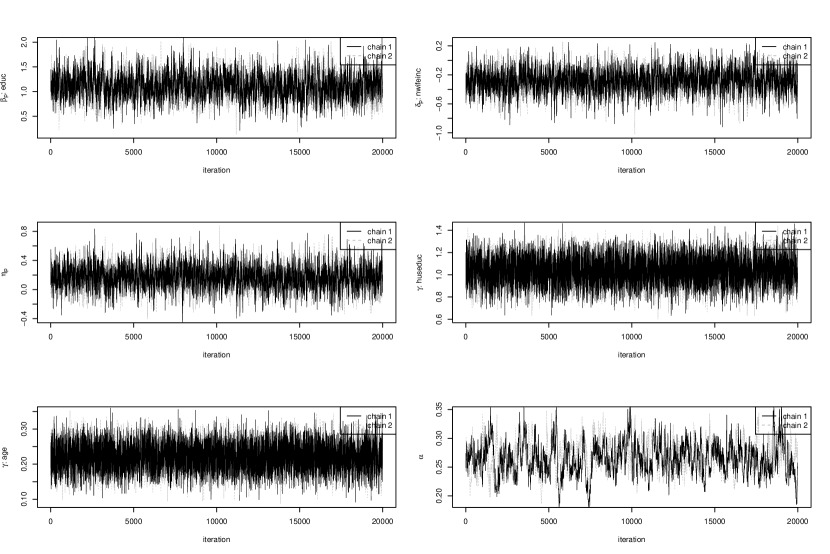
Figure 3: Post burn-in trace plots for SNDP for $p=0.1$

First, we present the results for the representative quantiles, $p=0.1$, $0.5$, and $0.9$. Table 4 shows the posterior means, 95% credible intervals, and inefficiency factors for ALDP and SNDP for these quantiles. The table shows that the sampling algorithm worked efficiently as the inefficiency factors are reasonably small. The posterior means for the instrument, huseduc, are positive and the 95% credible intervals do not include zero for all cases for both models, implying that huseduc is a valid instrument. For $p=0.5$, the posterior means for $\eta_{p}$ are $0.450$ and $0.446$ for ALDP and SNDP, respectively, and the 95% credible intervals do not include zero. Therefore, it is suggested that non-wife income be treated as an endogenous variable for the median regression.

Table 4: Posterior Summary for Female Labour Data

			ALDP				SNDP
$p$	Parameter		Mean	95% CI		IF	Mean	95% CI		IF
0.1	$\text{\boldmath{$\beta$}}_{p}$	constant	-4.205 [	-10.758,	2.430]	13.0	-4.340 [	-11.121,	2.288]	18.2
		educ	1.126 [	0.656,	1.599]	12.7	1.117 [	0.659,	1.614]	47.7
		age	-0.436 [	-0.565,	-0.311]	25.1	-0.424 [	-0.554,	-0.293]	37.0
		exper	1.070 [	0.731,	1.437]	41.3	1.051 [	0.723,	1.387]	92.3
		expersq	-0.019 [	-0.030,	-0.009]	24.7	-0.019 [	-0.029,	-0.009]	52.4
		kidslt6	-8.346 [	-11.145,	-5.949]	80.4	-8.296 [	-10.948,	-5.861]	65.6
		kigsge6	0.068 [	-0.487,	0.534]	31.7	0.045 [	-0.528,	0.512]	14.4
	$\delta_{p}$	nwifeinc	-0.284 [	-0.584,	0.010]	14.1	-0.279 [	-0.577,	0.007]	33.4
	$\eta_{p}$		0.176 [	-0.117,	0.473]	11.5	0.171 [	-0.125,	0.472]	27.8
	$\gamma$	constant	-10.117 [	-14.486,	-5.490]	9.4	-10.609 [	-15.023,	-6.112]	11.3
		huseduc	1.013 [	0.771,	1.239]	9.7	1.037 [	0.812,	1.257]	4.9
		educ	0.272 [	0.018,	0.551]	6.6	0.286 [	0.018,	0.562]	5.7
		age	0.210 [	0.140,	0.280]	6.7	0.221 [	0.152,	0.290]	7.6
		exper	-0.090 [	-0.269,	0.084]	12.2	-0.122 [	-0.301,	0.052]	8.5
		expersq	-0.003 [	-0.009,	0.003]	12.2	-0.002 [	-0.008,	0.003]	4.7
		kidslt6	-0.554 [	-1.424,	0.351]	6.4	-0.472 [	-1.430,	0.469]	5.5
		kigsge6	0.481 [	0.125,	0.838]	6.9	0.464 [	0.080,	0.839]	7.7
	$\alpha$		0.250 [	0.211,	0.298]	33.9	0.265 [	0.212,	0.322]	78.7
0.5	$\text{\boldmath{$\beta$}}_{p}$	constant	8.571 [	-0.899,	17.634]	7.1	8.265 [	-1.288,	17.473]	9.1
		educ	1.287 [	0.734,	1.889]	11.0	1.291 [	0.727,	1.895]	8.2
		age	-0.510 [	-0.680,	-0.333]	10.9	-0.502 [	-0.670,	-0.321]	12.9
		exper	1.398 [	1.029,	1.787]	12.0	1.391 [	1.021,	1.777]	12.1
		expersq	-0.021 [	-0.034,	-0.009]	13.4	-0.021 [	-0.034,	-0.009]	13.3
		kidslt6	-9.546 [	-11.975,	-7.305]	14.5	-9.441 [	-11.849,	-7.123]	5.2
		kigsge6	-0.255 [	-1.116,	0.620]	10.9	-0.268 [	-1.104,	0.592]	10.4
	$\delta_{p}$	nwifeinc	-0.525 [	-0.944,	-0.159]	15.5	-0.522 [	-0.917,	-0.165]	8.5
	$\eta_{p}$		0.450 [	0.079,	0.885]	14.0	0.446 [	0.087,	0.852]	7.9
	$\gamma$	constant	-10.318 [	-14.784,	-5.689]	12.3	-11.021 [	-15.556,	-6.377]	11.2
		huseduc	1.013 [	0.768,	1.242]	9.7	1.032 [	0.809,	1.251]	7.7
		educ	0.277 [	0.025,	0.557]	5.8	0.301 [	0.028,	0.583]	5.5
		age	0.212 [	0.142,	0.283]	8.2	0.226 [	0.156,	0.296]	11.5
		exper	-0.090 [	-0.274,	0.084]	4.3	-0.120 [	-0.298,	0.054]	9.4
		expersq	-0.003 [	-0.009,	0.003]	4.4	-0.002 [	-0.008,	0.003]	8.4
		kidslt6	-0.536 [	-1.408,	0.362]	2.9	-0.447 [	-1.413,	0.515]	3.1
		kigsge6	0.491 [	0.136,	0.850]	2.7	0.468 [	0.082,	0.863]	4.9
	$\alpha$		0.250 [	0.212,	0.297]	18.6	0.263 [	0.215,	0.315]	77.0
0.9	$\text{\boldmath{$\beta$}}_{p}$	constant	17.077 [	9.225,	25.430]	7.5	16.957 [	8.985,	25.429]	3.2
		educ	0.405 [	-0.107,	0.905]	7.9	0.420 [	-0.102,	0.921]	2.1
		age	-0.266 [	-0.424,	-0.112]	6.7	-0.265 [	-0.419,	-0.113]	2.7
		exper	1.075 [	0.749,	1.387]	13.1	1.072 [	0.747,	1.389]	12.0
		expersq	-0.018 [	-0.026,	-0.010]	10.8	-0.018 [	-0.026,	-0.010]	8.8
		kidslt6	-6.014 [	-8.373,	-3.553]	7.9	-6.085 [	-8.476,	-3.584]	8.3
		kigsge6	0.254 [	-0.490,	0.978]	5.7	0.254 [	-0.492,	1.009]	9.9
	$\delta_{p}$	nwifeinc	-0.043 [	-0.384,	0.288]	4.5	-0.050 [	-0.380,	0.275]	6.7
	$\eta_{p}$		-0.002 [	-0.340,	0.339]	5.0	0.004 [	-0.328,	0.337]	6.8
	$\gamma$	constant	-10.174 [	-14.698,	-5.486]	6.1	-10.741 [	-15.390,	-5.946]	16.1
		huseduc	1.013 [	0.773,	1.240]	9.2	1.036 [	0.812,	1.253]	6.3
		educ	0.274 [	0.021,	0.551]	9.5	0.292 [	0.017,	0.582]	9.5
		age	0.211 [	0.138,	0.283]	4.2	0.223 [	0.151,	0.294]	14.0
		exper	-0.092 [	-0.272,	0.085]	5.8	-0.126 [	-0.300,	0.048]	6.9
		expersq	-0.003 [	-0.009,	0.003]	7.0	-0.002 [	-0.008,	0.003]	6.0
		kidslt6	-0.550 [	-1.435,	0.349]	7.2	-0.483 [	-1.450,	0.500]	9.5
		kigsge6	0.483 [	0.128,	0.837]	4.3	0.464 [	0.076,	0.857]	4.2
	$\alpha$		0.251 [	0.213,	0.291]	34.5	0.265 [	0.213,	0.321]	66.1

To study the endogeneity in non-wife household income across quantiles, the posterior distributions of $\eta_{p}$ are presented. The results across the quantiles can be best understood by plotting the posterior distributions as a function of $p$. Figure 4 shows the posterior means and 95% credible intervals of $\eta_{p}$ for ALDP and SNDP for $p=0.05,0.1,\dots,0.95$. The figure shows that the two models produced similar results and that the posterior distributions of $\eta_{p}$ are concentrated away from zero for the mid quantiles. Specifically, for $0.2<p<0.65$, the 95% credible intervals do not include zero for either model. There are notable peaks around $p=0.35$, where the posterior means of $\eta_{p}$ under the default prior specifications are $0.664$ and $0.662$ with the 95% credible intervals $(0.201,1.137)$ and $(0.230,1.124)$ for ALDP and SNDP, respectively. This is an interesting result considering that the censoring rate is $0.43$. The result implies that the effect of the endogeneity of non-wife income is the most profound when the wife is about to decide whether to enter the labour force. When the opportunity cost of labour supply is very high (lower quantile) or the wife works on a more regular basis (higher quantile), such endogeneity diminishes. Smith and Blundell (1986) also reported that non-wife income is endogenous by using the endogenous Tobit regression model. The mean of our dataset is $7.399$, which approximately corresponds to the $0.6$-th quantile. For $p=0.6$, the posterior mean of $\eta_{p}$ for ALDP is $0.428$ with the 95% credible interval $(0.036,0.832)$ and that for SNDP is $0.421$ with the 95% credible interval $(0.037,0.832)$. The figure also shows the posterior means and 95% credible intervals under the two alternative prior specifications considered in Section 4.3, confirming that our results are robust with respect to the prior specifications.

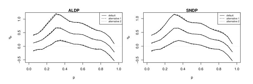
Figure 4: Posterior means and 95% credible intervals of $\eta_{p}$ under the default and alternative priors for $p=0.05,0.1,\dots,0.95$

Figure 5 compares the posterior means and 95% credible intervals of $(\text{\boldmath{$\beta$}}_{p}^{\prime},\delta_{p})^{\prime}$ for SNDP, ALDP, and TQR for $p=0.05,0.1,\dots,0.95$. The results for SNDP and ALDP are quite similar. The figure clearly shows that the posterior distributions for the key variable, nwifeinc, for the proposed models and TQR exhibit some differences for $0.2<p<0.65$, where nwifeinc is indicated to be endogenous. The difference becomes the most profound around $p=0.35$ for which the posterior mean for nwifeinc is $-0.761$ for ALDP, $-0.756$ for SNDP, and $-0.147$ for TQR, implying a stronger effect of non-wife income when endogeneity is taken into account. The posterior distributions for nwifeinc for ALDP and SNDP are more dispersed than that for TQR for all $p$. While the 95% credible intervals include zero for all models for the upper quantiles, for the lower quantiles, such as $p=0.1$, those for ALDP and SNDP include zero and those for TQR do not.

Differences in the results are also observed for other variables. For $p=0.35$, the posterior means for educ and age are respectively $1.689$ and $-0.513$ for ALDP, $1.705$ and $-0.504$ for SNDP, and $1.064$ and $-0.606$ for TQR. For the upper quantiles, $p>0.85$, the 95% credible intervals for educ include zero for the proposed models, while those for TQR do not, implying that an additional year of education does not increase the working hours for those quantiles when the endogeneity from non-wife income is taken into account. For expersq, the endogenous models result in slightly more dispersed posterior distributions for $0.2<p<0.7$. The posterior means for $p=0.35$ are $-0.021$, $-0.020$, and $-0.016$ for ALDP, SNDP, and TQR, respectively. For kidsge6, the posterior means for $p=0.35$ are $-0.274$, $-0.262$, and $-0.475$ for ALDP, SNDP, and TQR, respectively. However, the 95% credible intervals include zero for all $p$ for all models. On the other hand, the figure also shows that the models produced similar results for exper and kidslt6 for all $p$.

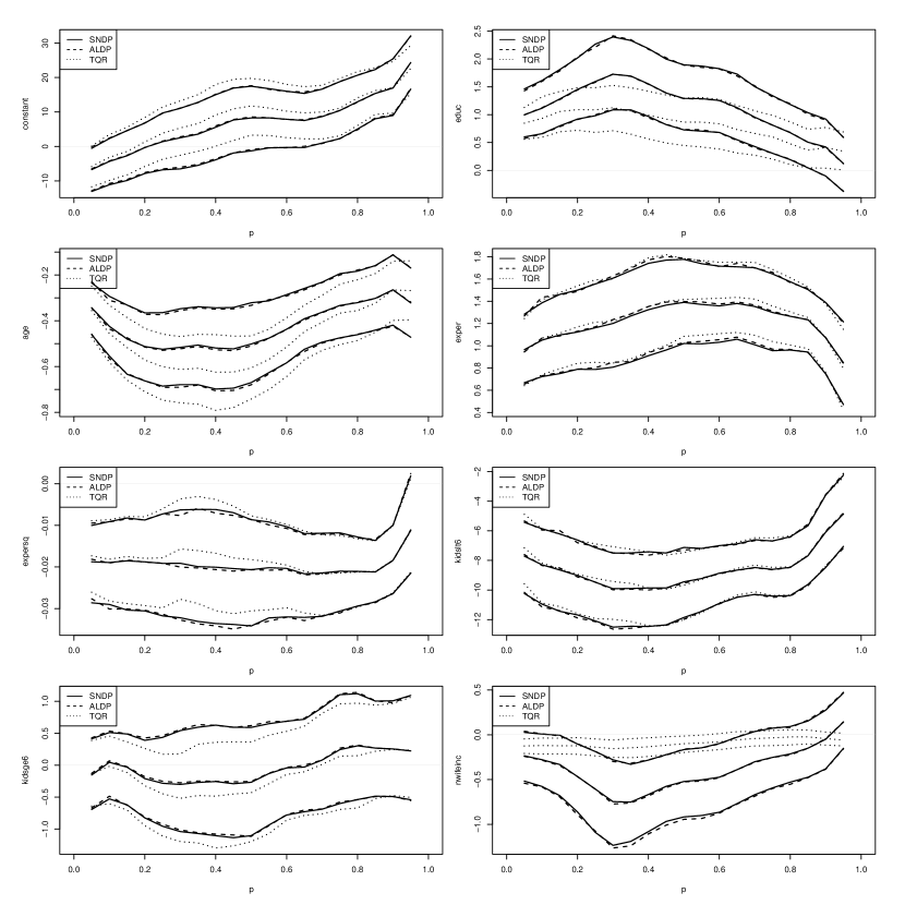
Figure 5: Posterior means and 95% credible intervals of $(\text{\boldmath{$\beta$}}_{p}^{\prime},\delta_{p})^{\prime}$ for ALDP, SNDP, and TQR for $p=0.05,0.1,\dots,0.95$

6 Conclusion

We proposed Bayesian endogenous TQR models using parametric and semiparametric first stage regression models built around the zero $\alpha$-th quantile assumption. The value of $\alpha$ determines the quantile level of the mode of the error distribution and is estimated from the data. From the simulation study, the AL, ALDP, and SNDP models worked relatively well for the various situations, while they faced the same limitation pointed out by Kottas and Krnjajić (2011). On the other hand, the SN model could not accommodate the fat tailed first stage errors. Although AEP could be a promising model in terms of flexibility, the inefficiency of the MCMC algorithm largely limits its applicability in practice. The development of a more convenient mixture representation for the AEP distribution is thus required. From application to data on the labour supply of married women, the effect of the endogeneity in non-wife income was found to be the most profound for the quantile level close to the censoring rate. For this quantile, some differences in the parameter estimates between the endogenous and standard models were found, such as the stronger effect of non-wife income on working hours.

This study only considered the case of continuous endogenous variables. We are also interested in incorporating endogenous binary variables into a Bayesian quantile regression model. An important extension might therefore be addressing multiple endogenous dummy variables to represent selection among multiple alternatives, such as the choice of a hospital and insurance plan, as considered in Geweke et al. (2003) and Deb et al. (2006). However, such an extension would be challenging with respect to the assumptions that must be imposed on the multivariate error terms. We leave these issues to future research.

Acknowledgements

The author would like to thank the seminar participants at the second BAYSM and ESOBE 2014 and the anonymous referees for the valuable comments to improve the manuscript. The computational results were obtained by using Ox version 6.21 (Doornik, 2007). This study was supported by JSPS KAKENHI Grant Numbers 25245035, 26245028, 26380266, and 15K17036.

References

- [1] Alhamzawi, R. (2014). “Bayesian elastic net Tobit quantile regression,” Communications in Statistics - Simulation and Computation, DOI:10.1080/03610918.2014.904341.
- [2] Alhamzawi, R. and Yu, K. (2014). “Bayesian Tobit quantile regression using g-prior distribution,” Journal of Statistical Computation and Simulation, DOI:10.1080/00949655.2014.945449.
- [3] Amemiya, T. (1979). “The estimation of a simultaneous equation Tobit model,” International Economic Review, 20, 169–181.
- [4] Amemiya, T. (1982). “Two stage least absolute deviations estimators,” Econometrica, 50, 689–771.
- [5] Abadie, A., Angrist, J. D., and Imbens, G. W. (2002). “Instrumental variable estimates of the effect of subsidized training on the quantiles of trainee earnings,” Econometrica, 70, 91–117.
- [6] Azzalini, A. and Capitanio, A. (2003). “Distributions generated by perturbation of symmetry with emphasis on a multivariate skew -distribution,” Journal of Royal Statistical Society Series B, 65, 367–389.
- [7] Barndorff-Nielsen, O. E. and Shephard, N. (2001). “Non-Gaussian Ornstein-Uhlenbeck-based models and some of their uses in financial econometrics,” Journal of Royal Statistical Society Series B, 63, 167–241.
- [8] Bilias, Y., Chen, S., and Ying, Z. (2000). “Simple resampling methods for censored regression quantiles,” Journal of Econometrics, 68, 303–338.
- [9] Blundell, R. W. and Smith, R. J. (1989). “Estimation in a class of simultaneous equation limited dependent variable models,” Review of Economic Studies, 56, 37–57.
- [10] Blundell, R. W. and Powell, J. L. (2007). “Censored regression quantiles with endogenous regressors,” Journal of Econometrics, 141, 65-83.
- [11] Buchinsky, M. (1998). “Recent advances in quantile regression models: a practical guide for empirical research,” Journal of Human Resources, 33, 88–126.
- [12] Buchinsky, M. and Hahn, H. (1998). “An alternative estimator for censored quantile regression,” Econometrica, 66, 653–671.
- [13] Chen, S. (2010). “An integrated maximum score estimator for a generalized censored quantile regression model,” Journal of Econometrics, 155, 90–98.
- [14] Chernozhukov, V. and Hong, H. (2002). “Three-step censored quantile regression and extramarital affairs,” Journal of the American Statistical Association, 97, 872–882.
- [15] Chernozhukov, V. and Hong, H. (2003). “An MCMC approach to classical estimation,” Journal of Econometrics, 115, 293–346.
- [16] Chernozhukov, V. and Hansen, C. (2005). “An IV model of quantile treatment effects,” Econometrica, 73, 245–261.
- [17] Chernozhukov, V. and Hansen, C. (2006). “Instrumental quantile regression inference for structural and treatment effect models”, Journal of Econometrics, 132, 491–525.
- [18] Chernozhukov, V. and Hansen, C. (2008). “Instrumental variable quantile regression: a robust inference approach,” Journal of Econometrics, 142, 379–398.
- [19] Chernozhukov, V., Fernández-Val, I., and Melly, B. (2013). “Inference on counterfactual distributions,” Econometrica, 81, 2205–2268.
- [20] Chernozhukov, V., Fernández-Val, I., and Kowalski, A. E. (2014). “Quantile regression with censoring and endogeneity,” Journal of Econometrics, doi:10.1016/j.econom.2014.06.017.
- [21] Chib, S. (2001). “Markov chain Monte Carlo methods: Computation and inference,” in J.J. Heckman and E. Leamer (eds.), Handbook of Econometrics 5, 3569–3649, North Holland: Amsterdam.
- [22] Conely, T. G., Hansen, C. B., McCulloch, R. E., and Rossi, P. E. (2008). “A semi-parametric Bayesian approach to the instrumental variable problem,” Journal of Econometrics, 144, 276–305.
- [23] Deb, P., Munkin, K. M., and Trivedi, K. P. (2006). “Bayesian analysis of the two-part model with endogeneity: application to health care expenditure,” Journal of Applied Econometrics, 21, 1081–1099.
- [24] Doornik, J. (2007). Ox: Object Oriented Matrix Programming, Timberlake Consultants Press: London.
- [25] Frhwirth-Schnatter, S. and Pyne, D. (2010). “Bayesian inference for finite mixtures of univariate and multivariate skew-normal and skew- distributions,” Biostatistics, 11, 317–336.
- [26] Gelman, A., Carlin, J. B., Stern., H. S., Dunson, D. B., Vehtari, A., and Rubin, D. B. (2014). Bayesian Data Analysis Third Edition, CRC Press: Boca Raton.
- [27] Geweke, J., Gowrisankaran, G., and Town, R. J. (2003). “Bayesian inference for hospital quality in a selection model,” Econometrica, 71, 1215–1238.
- [28] Hahn, J. (1995). “Bootstrapping quantile regression estimators,” Econometric Theory, 11, 105–121.
- [29] Heckman, J. J. (1978). “Dummy endogenous variables in a simultaneous equation system,” Econometrica, 46, 931–959.
- [30] Hoogerheide, L. F., Kleibergen, F., van Dijk, H. K. (2007a). “Natural conjugate priors for the instrumental variables regression model applied to the Angrist-Krueger data,” Journal of Econometrics138, 63–103.
- [31] Hoogerheide, L., Kaashoek, J. F., and van Dijk, H. K. (2007b). “On the shape of posterior densities and credible sets in instrumental variable regression models with reduced rank: An application of flexible sampling methods using neural networks,” Journal of Econometrics, 139, 154–180.
- [32] Ishwaran, H. and James, L. F. (2002). “Approximate Dirichlet process computing in finite normal mixtures: smoothing and prior information,” Journal of Computational and Graphical Statistics, 11, 508–532.
- [33] Ji, Y., Lin, N., and Zhang, B. (2012). “Model selection in binary and Tobit quantile regression using the Gibbs sampler,” Computational Statistics & Data Analysis, 56, 827–839.
- [34] Kim, T. H., and Muller C. (2004). “Two-stage quantile regression when the first stage is based on quantile regression,” Econometrics Journal, 7, 218–231.
- [35] Kobayashi, G. and Kozumi, H. (2012). “Bayesian analysis of quantile regression for censored dynamic panel data,” Computational Statistics, 27, 359–380.
- [36] Kobayashi, G. (2015). “Skew exponential power stochastic volatility model for analysis of skewness, non-normal tails, quantiles and expectiles,” Computational Statistics, DOI:10.1007/s00180-015-0596-4.
- [37] Koenker, R. and Bassett, G. (1978). “Regression quantiles,” Econometrica, 46, 33–50.
- [38] Koenker, R. and Machado, J. A. F. (1999). “Goodness of fit and related inference processes for quantile regression,” Journal of the American Statistical Association, 94, 1296–1310.
- [39] Koenker, R. (2005). Quantile Regression, Cambridge University Press, New York.
- [40] Kottas, A. and Gelfand, A. E. (2001). “Bayesian semiparametric median regression modeling,” Journal of the American Statistical Association, 96, 1458–1467.
- [41] Kottas, A., Krnjajić, M. (2009). “Bayesian semiparametric modelling in quantile regression,” Scandinavian Journal of Statistics, 36, 297–319.
- [42] Kotz,S., Kozubowski, T. J., and Podgòrski, K. (2001). The Laplace Distribution and Generalizations: A Revisit with Applications to Communications, Economics, Engineering, and Finance, Birkhuser, Boston.
- [43] Kozumi, H. and Kobayashi, G. (2011). “Gibbs sampling methods for Bayesian quantile regression,” Journal of Statistical Computation and Simulation, 81, 1565–1578.
- [44] Lancaster, T. and Jun, S. J. (2010). “Bayesian quantile regression methods,” Journal of Applied Econometrics, 25, 287–307.
- [45] Lee, S. (2007). “Endogeneity in quantile regression models: a control function approach,” Journal of Econometrics, 141, 1131-1158.
- [46] Lin, G., He, X., Pornoty, S. (2012). “Quantile regression with doubly censored data,” Computational Statistics & Data Analysis, 2012, 797–812.
- [47] Lopes, H. F. and Polson, N. G. (2014). “Bayesian instrumental variables: Priors and likelihoods,” Econometric Reviews, 33, 100–121.
- [48] Ma, L. and Koenker, R. (2006). “Quantile regression methods for recursive structural equation models,” Journal of Econometrics, 134, 471–506.
- [49] Mroz, T. (1987). “The sensitivity of an empirical model of married women’s hours of work to economic and statistical assumptions,” Econometrica, 55, 765–799.
- [50] Munkin, M. K. and Trivedi, P. K. (2003). “Bayesian analysis of a self-selection model with multiple outcomes using simulation-based estimation: an application to the demand for healthcare,” Journal of Econometrics, 114, 197–220.
- [51] Munkin, M. K. and Trivedi, P. K. (2008). “Bayesian analysis of the ordered probit model with endogenous selection,” Journal of Econometrics, 143, 334–348.
- [52] Naranjo, L., Pérez, C. J., and Martín, J. (2015). “Bayesian analysis of some models that use the asymmetric exponential power distribution,” Statistics and Computing, 25, 497–514.
- [53] Nelson, F. and Olsen, L. (1978). “Specification and estimation of a simultaneous equation model with limited dependent variables,” International Economic Review, 19, 659–705.
- [54] Newey, W. K. (1987). “Efficient estimation of limited dependent variable models with endogenous explanatory variables,” Journal of Econometrics, 36, 231–250.
- [55] Ogasawara, K. and Kobayashi, G. (2015). “The impact of social workers on infant mortality in inter-war Tokyo: Bayesian dynamic panel quantile regression with endogenous variables,” Cliometrica, 9, 97–130.
- [56] Papaspiliopoulos, O. and Roberts, G. O. (2008). “Retrospective MCMC for Dirichlet process hierarchical models,” Biometrika, 95, 169–186.
- [57] Powell, J. L. (1983). “The asymptotic normality of two-stage least absolute deviations estimators,” Econometrica, 51, 1569–1576.
- [58] Powell, J. L. (1984). “Least absolute deviations estimation for the censored regression model,” Journal of Econometrics, 20, 303-325.
- [59] Powell, J. L. (1986). “Censored regression quantiles,” Journal of Econometrics, 32, 143-155.
- [60] Rossi, P. E., Allenby, G. M., and McCulloch, R. (2005). Bayesian Statistics and Marketing, Wiley: New York.
- [61] Reich, B. J., Bondell, H. D., and Wang, H. J. (2010). “Flexible Bayesian quantile regression for independent and clustered data,” Biostatistics, 11, 337–352.
- [62] Reich, B. J. and Smith, L. B. (2013). “Bayesian quantile regression for censored data,” Biometrics, 68, 651–660.
- [63] Sethuraman, J. (1994). “A constructive definition of Dirichlet priors,” Statistica Sinica, 4, 639–650.
- [64] Smith, R. J. and Blundell, R. W. (1986). “An exogeneity test for a simultaneous equation Tobit model with an application to labor supply,” Econometrica, 56, 679–685.
- [65] Sriram, K., Ramamoorthi, R. V., and Ghosh, P. (2013). “Posterior consistency of Bayesian quantile regression based on the misspecified asymmetric Laplace density,” Bayesian Analysis, 8, 479–504.
- [66] Taddy, A. M. and Kottas, A. (2010). “A Bayesian nonparametric approach to inference for quantile regression,” Journal of the American Statistical Association, 28, 357–369.
- [67] Tang, Y., Wang, H. J., He, X., and Zhu, Z. (2012). “An informative subset-based estimator for censored quantile regression,” Test, 21, 635–655.
- [68] Walker, S. (2007). “Sampling the Dirichlet mixture model with slices,” Communications in Statistics - Simulation and Computation, 36, 45–54.
- [69] Wang, H. J. and Fygenson, M. (2009). “Inference for censored quantile regression models in longitudinal studies,” The Annals of Statistics, 37, 756–781.
- [70] Wang, H. J. and Wang, L. (2009). “Locally weighted censored quantile regression,” Journal of the American Statistical Association, 104, 1117–1128.
- [71] Wichitaksorn, N., Choy, S. T. B., and Gerlach, R. (2014). “A generalized class of skew distributions and associated robust quantile regression models,” The Canadian Journal of Statistics, 42, 5779–596.
- [72] Xie, S., Wan, A. T. K., and Zhou, Y. (2015). “Quantile regression methods with varying-coefficient models for censored data,” Computational Statistics & Data Analysis, 88, 154–172.
- [73] Yu, K. and Moyeed, R. A. (2001). “Bayesian quantile regression,” Statistics and Probability Letters, 54, 437–447.
- [74] Yu, K., Lu, Z., and Stander, J. (2003). “Quantile regression: applications and current research areas,” Statistician, 52, 331–350.
- [75] Yu, K. and Zhang, J. (2005). “A three-parameter asymmetric Laplace distribution and its extension,” Communications in Statistics - Theory and Methods, 34, 1867–1879.
- [76] Yu, K. and Stander, J. (2007). “Bayesian analysis of a Tobit quantile regression model,” Journal of Econometrics, 137, 260-276.
- [77] Zhao, K. and Lian, H. (2015). “Bayesian Tobit quatile regression with single-index models,” Journal of Statistical Computation and Simulation, 85, 1247–1263.
- [78] Zhu, D. and Zinde-Walsh, V. (2009). “Properties and estimation of asymmetric exponential power distribution,” Journal of Econometrics, 148, 86–99.
- [79] Zhu, D. and Galbraith, J. W. (2011). “Modeling and forecasting expected shortfall with the generalized asymmetric Student- and asymmetric exponential power distributions,” Journal of Empirical Finance, 18, 765–778.