Are the total mass density and the low-mass end slope of the IMF anti-correlated?

Abstract

We conduct a detailed lensing, dynamics and stellar population analysis of nine massive lens early-type galaxies (ETGs) from the X-Shooter Lens Survey (XLENS). Combining gravitational lensing constraints from HST imaging with spatially-resolved kinematics and line-indices constraints from VLT X-Shooter (XSH) spectra, we infer the low-mass slope and the low cut-off mass of the stellar Initial Mass Function (IMF): $x_{250}=2.37^{+0.12}_{-0.12}$ and $M_{\mathrm{low},250}=0.131^{+0.023}_{-0.026}\,M_{\odot}$, respectively, for a reference point with $\sigma_{\star}\equiv 250\,\mathrm{km\,s^{-1}}$ and $R_{\rm eff}$$\equiv 10$ kpc. All the XLENS systems are consistent with an IMF slope steeper than Milky Way-like. We find no significant correlations between IMF slope and any other quantity, except for an anti-correlation between total dynamical mass density and low-mass IMF slope at the 87% CL [$dx/d\log(\rho)$ = $-0.19^{+0.15}_{-0.15}$]. This anti-correlation is consistent with the low redshift lenses found by Smith et al. (2015) that have high velocity dispersions and high stellar mass densities but surprisingly shallow IMF slopes.

1 Introduction

Low mass stars ($M\leq 0.3\,M_{\odot}$) contribute at most 5–10 per cent to the total optical light of the integrated spectrum of early-type galaxies (ETGs) but dominate the total stellar mass budget (Worthey 1994). Variations in the number of M-dwarfs can therefore dramatically change the stellar mass-to-light ratio ($\Upsilon_{\star}$) without significantly affecting the characteristics of the observed light (e.g., Bell & de Jong 2001; Conroy & van Dokkum 2012a; Conroy 2013). Hence the initial mass function (IMF), and especially its low-mass slope, plays a fundamental role in determining an ETG’s $\Upsilon_{\star}$ and is crucial to understand the internal structure, the formation times and the evolution of these massive galaxies (e.g. Blumenthal et al. 1984), providing important insight into galaxy evolution mechanisms (e.g. Padmanabhan et al. 2004; Tortora et al. 2009; Auger et al. 2010; Graves & Faber 2010; Barnabè et al. 2011).
Recent observations, based on gravitational lensing, dynamics and/or simple stellar population (SSP) modeling of galaxy spectra, indicate that the number of low-mass stars in the central region of ETGs increases rapidly with stellar velocity dispersion (Treu et al. 2010; van Dokkum & Conroy 2010; Spiniello et al. 2011, 2012; Cappellari et al. 2012; La Barbera et al. 2013; Tortora, Romanowsky & Napolitano 2013; Spiniello et al. 2014; Martín-Navarro et al. 2015). Recently, however, Smith, Lucey & Conroy (2015, hereafter S15) presented results on three very massive lens ETGs with high velocity dispersions ($\sigma>300$ $\mathrm{km\,s^{-1}}$) and $\alpha$-enhanced abundances whose $\Upsilon_{\star}$ are compatible with a Milky Way-like IMF slope (although a Salpeter IMF cannot be excluded). The potential tension between different studies could indicate that stellar mass (or velocity dispersion) is not the main driver behind IMF variations, but only a proxy for other, more physically motivated causes.
[ caption = Properties of the nine XLENS systems used in the analysis., star, label = xlensintro_obsSLACS ]llllllll [ ]1) Based on WFPC2 F606W observations. 2) Luminosity-weighted stellar kinematics of the lens extracted from a rectangular aperture of $2\arcsec\times 1\aas@@fstack{\prime\prime}5$ centered on the galaxy’s center. See Paper II. 3) Best-fit IMF slope from spectroscopic, line-index based SSP analysis. For three systems, the spectra do not have S/N high enough to securely constrain the IMF. XLENS System z_lens z_source $R_{\rm eff}$(kpc) $R_{\rm Ein}$ (kpc) $L_{\rm V}$ ($10^{11}L_{\odot})^{1}$ $\sigma_{\rm XSH}$ (km/s)² IMF slope³
SDSSJ0037$-$0942 0.1955 0.6322 7.03 4.95 $1.09\pm 0.06$ $277\pm 6$ $2.5\pm 0.25$
SDSSJ0044$+$0113 0.1196 0.1965 5.56 1.72 $0.61\pm 0.05$ $260\pm 8$ $-$
SDSSJ0216$-$0813 0.3317 0.5235 12.6 5.53 $1.82\pm 0.05$ $327\pm 19$ $2.9\pm 0.35$
SDSSJ0912$+$0029 0.1642 0.3239 10.8 4.58 $1.47\pm 0.05$ $325\pm 10$ $2.6\pm 0.30$
SDSSJ0935$-$0003 0.3475 0.4670 20.7 4.26 $2.07\pm 0.07$ $380\pm 22$ $-$
SDSSJ0936$+$0913 0.1897 0.5880 6.61 3.45 $0.83\pm 0.05$ $256\pm 18$ $-$
SDSSJ0946$+$1006 0.2219 0.6085 8.33 4.95 $0.66\pm 0.06$ $300\pm 22$ $2.1\pm 0.15$
SDSSJ1143$-$0144 0.1060 0.4019 9.21 3.27 $0.95\pm 0.05$ $287\pm 18$ $2.4\pm 0.18$
SDSSJ1627$-$0053 0.2076 0.5241 6.66 4.18 $0.79\pm 0.05$ $303\pm 23$ $2.3\pm 0.26$
Strong gravitational lensing combined with stellar dynamics (GL+D) allows one to measure stellar masses of galaxies independently from assumptions about their stellar IMF or knowledge of their stellar population. Therefore, when combined with a measurement of the galaxy luminosity, one obtains a measure of the value of $\Upsilon_{\star}$ which is a function of the IMF, allowing the latter to be constrained (e.g. Treu et al. 2010; Spiniello et al. 2011; Barnabè et al. 2012, 2013). Applications of GL+D have shown that the total $\Upsilon_{\star}$ of massive ETGs increases monotonically with the velocity dispersion of the galaxy (e.g. Grillo et al. 2009; Auger et al. 2010; Treu et al. 2010; Barnabè et al. 2011; Dutton, Mendel & Simard 2012). A steepening of the low-mass end of the stellar IMF with galaxy mass could therefore be largely responsible for this change in $\Upsilon_{\star}$, although a change in the dark matter (DM) fraction could also play a role (Auger et al. 2009).
With the X-Shooter Lens Survey (XLENS: Spiniello et al. 2011; Barnabè et al. 2013, hereafter B13) we aim to probe variations of the low-mass end of the IMF and disentangle stellar and DM in the internal region of lens ETGs, via a joint lensing+dynamics+stellar population analysis.
Except for B13, all studies to date have assumed that the lower mass limit of the IMF is constant, since varying this parameter does not strongly impact the spectra nor change the line-index measurements for any assumed IMF slope. Stars with masses below $\sim 0.15\,M_{\odot}$ are however critical to determine $\Upsilon_{\star}$. The only possible way to break this degeneracy is by obtaining a measurement of the total stellar mass from an independent method, which, as in B13, is provided by a combined lensing and dynamics analysis.
In this Letter we study the low-mass end properties of the stellar IMF, inferring its slope and its low-mass cut-off ($M_{\mathrm{low}}$) in nine massive lens ETGs, quadrupling the sample presented in B13, which we subsequently augment by three recently discovered low-redshift lenses (S15). These two sets allow us, for the first time, to study trends of the IMF parameters (slope and low-mass limit) with stellar velocity dispersion, effective radius and galaxy mass density.

2 Data Set and Analysis

The XLENS sample consists of eleven massive lens ETGs with $\sigma_{\star}=250-400$ $\mathrm{km\,s^{-1}}$, all with multi-band HST and VLT XSH data. Here we use nine out of eleven systems with the necessary total luminosity and high signal-to-noise (S/N) spectra. Characteristics of the systems used in this work are presented in Table 1.
For the GL+D analysis we make use of the high-resolution F814W images of the lens systems, originally selected from the Sloan Lens ACS Survey (SLACS, Bolton et al. 2008). For the SSP modeling, UVB–VIS high signal-to-noise spectra ($\mathrm{S/N}>50$) have been obtained during two runs between 2011 and 2013 in slit mode (UVB: $\mathrm{R}=3300$ with $1\aas@@fstack{\prime\prime}6\times 11\aas@@fstack{\prime\prime}$ slit; VIS: $\mathrm{R}=5400$, with $1\aas@@fstack{\prime\prime}5\times 11\aas@@fstack{\prime\prime}$ slit).
We refer to Paper II (Spiniello et al. 2015, submitted) for a more detailed presentation of the full survey sample and the spatially resolved kinematics analysis of the systems, to B13 for a detailed description of the precise methodology and to Paper III (Barnabè et al., in prep.) for a more extensive discussion and results of the GL+D analysis of the full sample as well as detailed constraints on the DM halo fraction and density profiles.

Figure 1: Marginalized posteriors for the model fitting of IMF slope ($x$) and cut-off mass ($M_{\mathrm{low}}$) as function of $\sigma$ and $R_{\mathrm{eff}}$ (in unit of $250$ $\mathrm{km\,s^{-1}}$ and 10 kpc, respectively), including the XLENS systems only (left, red contours) or the XLENS$+$S15 systems (right, blue contours).

To infer the IMF slope and cut-off mass, we apply the same methodology introduced in B13, summarized below.

i) From a GL+D analysis, we determine the posterior probability density function (PDF) of the stellar mass of each of the nine lens galaxies. This measurement is independent from any SSP or photometric analysis and does not make any assumption about the IMF. As in B13, we use the fully Bayesian CAULDRON code (detailed in Barnabè & Koopmans 2007 and Barnabè et al. 2012) which is designed to conduct a self-consistent combined modelling of both the lensing and kinematic constraints. In particular we use a flexible two-component axially-symmetric mass model for each lens. We use a generalized Navarro-Frenk-White (gNFW) for the DM halo profile, consistent with cosmological simulation findings, as well as observations, and we infer the density profile of the luminous mass component by deprojecting the multi-Gaussian expansion (MGE, Emsellem, Monnet & Bacon 1994; Cappellari 2002) fit to the observed surface brightness distribution of the galaxy. The total stellar mass then sets the normalization of the stellar mass distribution and is used to simultaneously model both the lensing data set and the stellar kinematic observables.
ii) We infer a value of the low-mass IMF slope from XSH spectra, using an extended version of the SSP models of Conroy & van Dokkum (2012a), as described in Spiniello et al. (2014) and Spiniello, Trager & Koopmans (2015). This inference (see Table 1) is used as Gaussian prior in our subsequent analysis. Only six out of nine ETGs have spectra that provide a solid measurement. For the three remaining systems, we assume a flat prior on the IMF slope between $x=1.8$ and $3.5$.
iii) We use a grid of $\Upsilon_{\star}$ values from the Dartmouth Stellar Evolution Program (Chaboyer et al. 2001) as functions of the IMF slope ($x=1.8-3.5$) and low-mass limit ($M_{\mathrm{low}}$$=0.01-0.22$). We use a Gaussian probability distribution function for total V-band luminosities ($L_{V}$) of the lens galaxies, as determined from HST data by Auger et al. (2009), to convert mass-to-light ratios ($\Upsilon_{\star}$) into stellar masses as function of the IMF slope and low-mass cut-off.
iv) We subsequently use a Markov Chain Monte Carlo (MCMC) analysis of the model parameters to derive the GL+D+SSP posterior PDFs of the IMF slope and low-mass cut-off for each lens galaxy. In the model, $x$, $M_{\rm low}$ and $L_{V}$ all vary. The GL+D PDFs for the stellar mass produce the likelihood, which we then multiply with the priors on luminosity and IMF slope from the HST and XSH data, respectively. Finally, the luminosity of the galaxy is marginalized out.
In this way, we obtain a posterior probability density for each system:

$$P(x,M_{\rm low}|{\rm data})=\int_{{\rm L}}{\cal{L}}({\rm data}_{{\rm GL+D}}|M_{*}=\Upsilon_{V}(x,M_{\rm low})\\ \times{\rm L}_{\rm V})\cdot P_{\rm HST}({\rm L}_{\rm V})\cdot P_{\rm SSP}(x)\cdot P(M_{\rm low})d{\rm L}_{\rm V}$$ (1)

With these nine $P(x,M_{\rm low}|{\rm data}_{i})$ in hand, which are kept fixed in the subsequent analysis, we proceed with inferring whether there are any trends of the IMF parameters with stellar velocity dispersion ($\sigma$) and effective radius ($R_{\rm eff}$) or the total (dynamical) density $\rho\equiv\sigma^{2}/R_{\rm eff}^{2}$. We first construct a multivariate model:

$$x=x_{250}+x^{\prime}_{1}\log_{10}(\sigma_{250})+x^{\prime}_{2}\log_{10}(R_{10})$$ (2)

$$M_{\mathrm{low}}=M_{\mathrm{low},250}+M_{\mathrm{low},1}^{{}^{\prime}}\log_{10}(\sigma_{250})+M_{\mathrm{low},2}^{{}^{\prime}}\log_{10}(R_{10})$$ (3)

where $x_{250}$ and $M_{\mathrm{low},250}$ represent the slope and the cut-off mass of the IMF respectively, and $\sigma_{250}$ and $R_{10}$ are the velocity dispersion in unit of $250$ $\mathrm{km\,s^{-1}}$ and the effective radius in units of 10 kpc.
We then sample, using a MCMC Metropolis algorithm, all six free parameters (the two biases and four trends with velocity dispersion and effective radius) and create their respective univariate and bivariate marginalised posteriors, assuming flat priors. The likelihood value is the product of the nine LHs values $\prod_{i=1,...9}P(x,M_{\mathrm{low}}|{\rm data}_{i})$ times the priors on the model parameters for the trend function inferred above (all assumed to be flat). The small measurements errors on the effective radius, velocity dispersion and redshift are negligible in this process. Each posterior is built from $10^{5}$ samples.
Besides the nine XLENS galaxies, we augmented the MCMC analysis with three high-velocity dispersion, low-redshift lenses presented in S15. Using their constraints on the $\Upsilon_{\star}$ and the ‘mass excess factor’ $\alpha$ (see Table 3 in S15), we infer the corresponding value of the IMF slope (unimodal, single power-law) for each galaxy. This produces a tightening of most of the marginalised posteriors, but there is no major shift in the results, indicating that the model is consistent with both data-sets and their combination.

Figure 2: 2-D marginalized PDFs for the model fitting of IMF slope ($x$) and low-mass cut-off ($M_{\mathrm{low}}$) as function of total density ($\rho=\sigma^{2}/R_{\mathrm{eff}}^{2}$) for the XLENS galaxies only (left, red contours) and for the XLENS+S15 sample (right, blue contours). The data suggest an anti-correlation between IMF slope and density.

3 MCMC Results

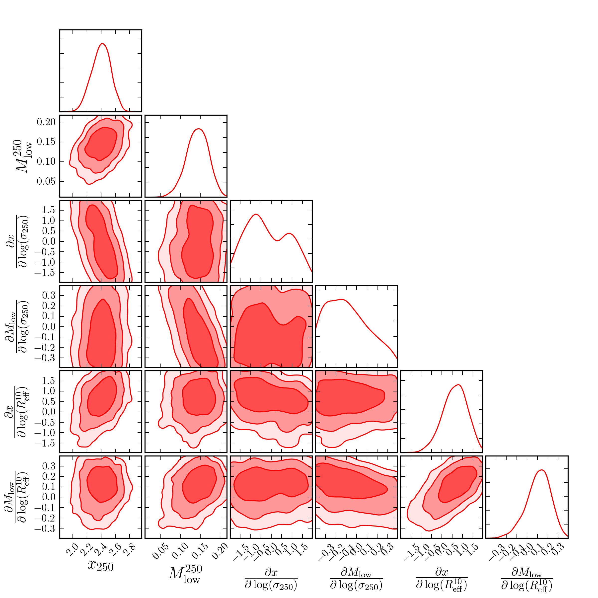
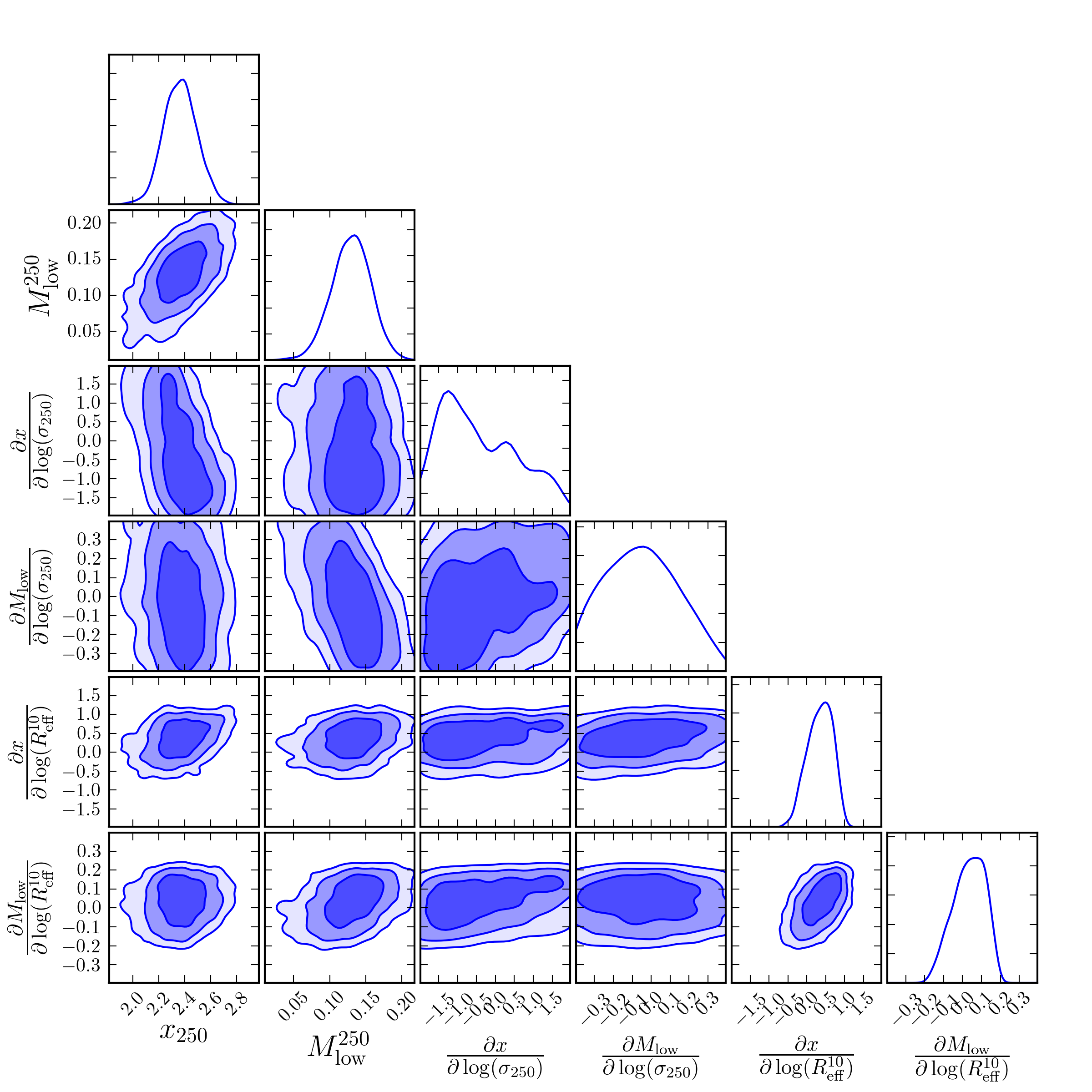
Figure 1 shows the univariate and bivariate marginalized posteriors resulting from the MCMC model fitting of the nine XLENS (left, red plots) and of the XLENS+S15 systems (right, blue plots). The upper panels of the first two columns show the bias values of the slope and the low-mass cut-off defined for a reference system with $\sigma\equiv 250$ $\mathrm{km\,s^{-1}}$ and $R_{\mathrm{eff}}\equiv 10$ kpc. We find $x_{250}$ = $2.41^{+0.11}_{-0.15}$ and $M_{\mathrm{low},250}$ = $0.144^{+0.024}_{-0.027}M_{\odot}$ for XLENS and $x_{250}$ = $2.37^{+0.12}_{-0.12}$ and $M_{\mathrm{low},250}$ = $0.131^{+0.023}_{-0.026}M_{\odot}$ for the XLENS+S15 case, respectively. The results are fully consistent. In both cases a Milky Way-like IMF ($x=1.8$) is ruled out with a high degree of confidence for our reference system, consistent with previous published results (B13, Cappellari et al. 2012; Conroy & van Dokkum 2012b; Spiniello et al. 2014). However, unlike previous results, we do not find any relation between the IMF slope and stellar velocity dispersion: $dx/d\log(\sigma)$ = $-0.36^{+1.40}_{-0.89}$ for XLENS and $dx/d\log(\sigma)$ = $-0.60^{+1.40}_{-0.89}$ for XLENS+S15. We note that the lack of a IMF-$\sigma$ relation does not necessarily contradict previous studies, since this is the first time in which both the IMF slope and IMF low-mass cut-off are treated as free parameters and the range of stellar velocity dispersions is relatively small ($280$-$380$ $\mathrm{km\,s^{-1}}$). If we force a trend of $x$ with $\sigma$, we must also have a trend of $M_{\mathrm{low}}$ with $\sigma$. This indicates a degeneracy between the IMF slope and the IMF low mass cut-off, as expected.
We find a marginally significant relation between IMF slope and effective radius: $dx/d\log(R_{\rm eff})$ = $0.66^{+0.51}_{-0.59}$ for XLENS and $dx/d\log(R_{\rm eff})$ = $0.37^{+0.32}_{-0.36}$ for XLENS+S15. We conclude, albeit with low significance, that the effective radius of ETGs might be a better indicator of IMF slope than their stellar velocity dispersion. Because in general the stellar dispersion correlates with effective radius, either can act as proxy for IMF slope, consistent with previous studies.

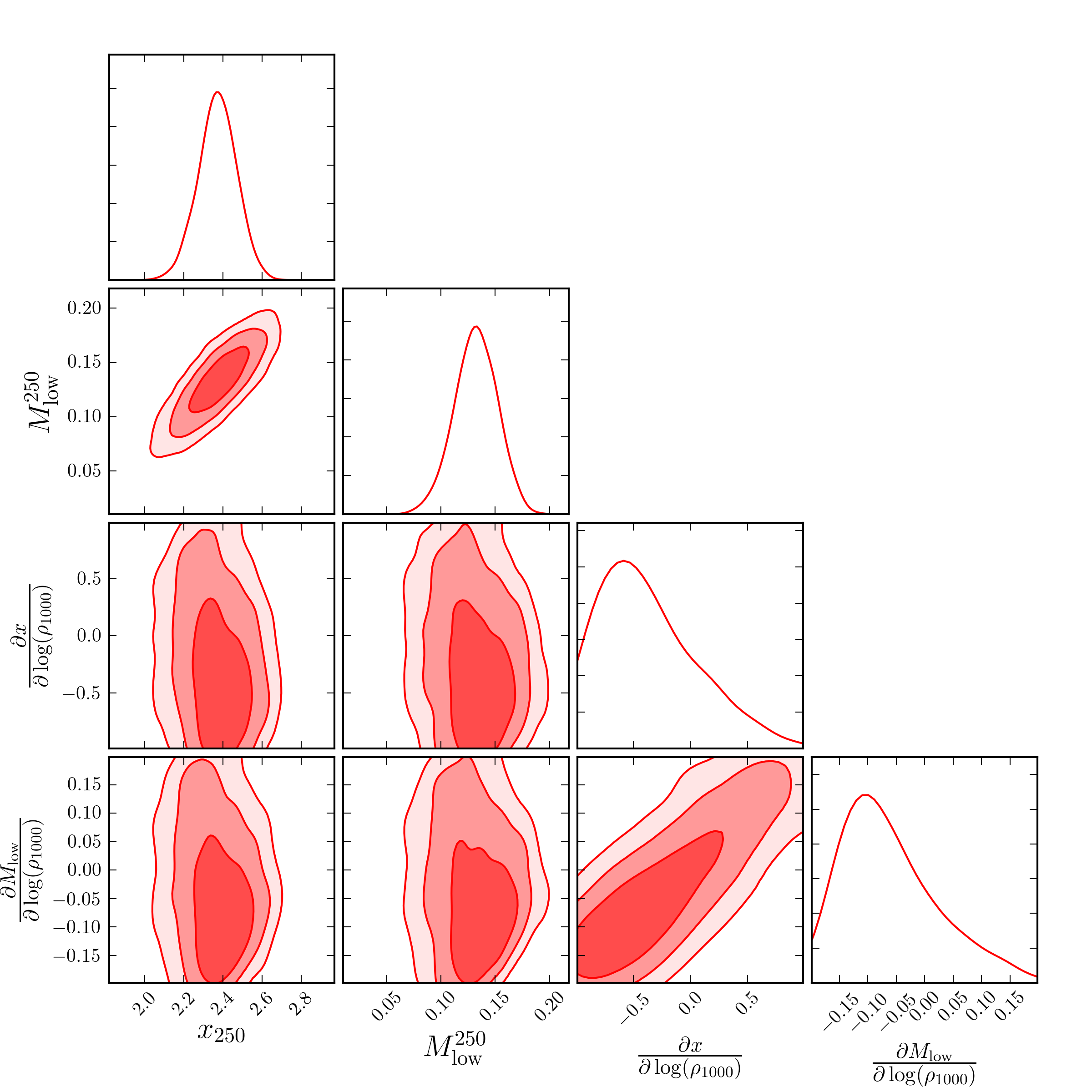
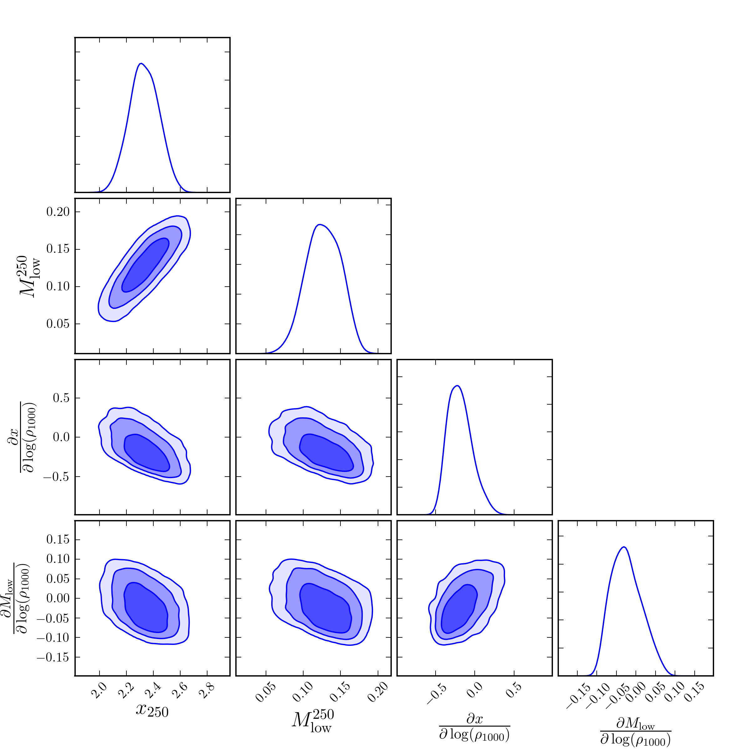
Since both velocity dispersion and effective radius are global parameters, they might only be proxies for the physical processes during star-formation. On the other hand, mass density might be a better indicator of the IMF slope and the low-mass cut-off. Figure 2 shows the marginalized posteriors resulting from a lower-dimensional MCMC power-law model fit where we define the total dynamical density as $\rho\propto\sigma^{2}/R_{\mathrm{eff}}^{2}$ in units of $1000$ $(\mathrm{km\,s^{-1}})^{2}/\textrm{kpc}^{2}$.
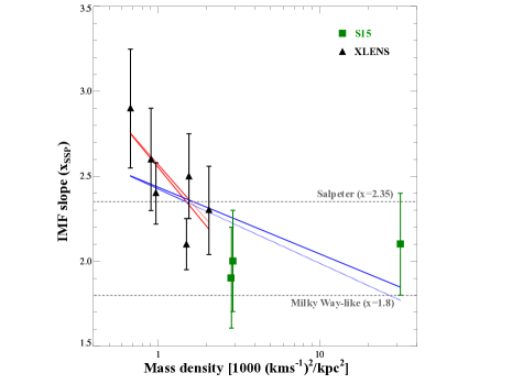
We find that total density anti-correlates with the IMF slope, i.e. steeper slopes for less dense stellar systems, and that the lower mass limit increases as well for less-dense systems: $dx/d\log(\rho)$ = $-0.47^{+0.55}_{-0.33}$ for XLENS only and $dx/d\log(\rho)$ = $-0.19^{+0.15}_{-0.15}$ for XLENS+S15 ($dx/d\log(\rho)<0$ at 87% CL). The relation is marginally significant, but when plotting the SSP-only inferred slopes of XLENS+S15 systems against total density (Fig. 3), we see that the S15 lenses are all much denser and extend the anti-correlation trend already seen from the XLENS systems. Moreover, $dx/d\log(\rho)$ obtained with a simple least-squares fit of the data (solid lines, red for XLENS only and blue for the XLENS+S15 case) agrees well with that obtained from the MCMC analysis (dotted lines, same color code), but we emphasize that these fits are only a sanity-check of the MCMC results.

4 Summary & Discussion

We combine the results of a state-of-the-art lensing and dynamics analysis of nine massive lens galaxies of the XLENS Survey with corresponding inferences from a spectroscopic SSP study of line-strength indices focusing on the properties of their IMFs. At the time of writing, this is the only method that allows the joint inference of the slope and low-mass cut-off of the IMF (see B13).
We use a multi-variate, six-dimensional Markov Chain Monte Carlo analysis to derive the GL+D+SSP posterior PDFs on trends of the IMF slope and low-mass cut-off with stellar velocity dispersion, effective radius and total mass density. The main results of our analysis are as follows:

1. For a reference galaxy with $\sigma\equiv 250$ $\mathrm{km\,s^{-1}}$ and $R_{\mathrm{eff}}\equiv 10$ kpc, we infer $x_{250}$ = $2.37^{+0.12}_{-0.12}$ and $M_{\mathrm{low},250}$ = $0.131^{+0.023}_{-0.026}$ $M_{\odot}$, consistent with the results previously published in B13 and with other published studies on massive ETGs.

2. A marginally significant correlation is found with the size of the galaxies, i.e. systems with larger $R_{\mathrm{eff}}$ prefer bottom-heavier IMFs. This correlation is similar to that with stellar velocity dispersion because more massive galaxies, statistically, also have larger effective radii.

3. We find an anti-correlation between IMF slope and total (dynamical) density, defined as $\rho=\sigma^{2}/R_{\mathrm{eff}}^{2}$. This trend could explain the seemingly contradictory result by Smith, Lucey & Conroy (2015) that suggests that some very high-velocity dispersion lenses have shallow IMFs slopes, counter to previous findings. Combining the XLENS+S15 sample, we find that the IMF slope anti-correlates (at 87% CL) with total mass density: $dx/d\log(\rho)$ = $-0.19^{+0.15}_{-0.15}$.

The fully Bayesian analysis of the IMF parameters using the XLENS systems confirms our previous results in B13 that the IMF slope is inconsistent with that of the Milky Way at a very high confidence level for reference galaxies with $\sigma\equiv 250$ $\mathrm{km\,s^{-1}}$  and $R_{\rm eff}$$\equiv 10$ kpc. We find marginal ($\sim 1$-$\sigma$) trends with effective radius and total mass-density. No trend with stellar velocity dispersion is found (although this is still consistent with our previous work). When we include the sample of S15, both trends become stronger; in particular the anti-correlation of the total mass density with IMF slope is found at the 87% CL. The S15 galaxies are much denser, with high stellar dispersion ($\sigma=[356\pm 16,356\pm 18,320\pm 18]$) but smaller effective radii ($R_{\rm eff,J}(kpc)=[6.6,2.0,6.0]$), than the XLENS galaxies. If indeed this trend with mass density is genuine, it explains the seemingly discrepant results between most studies and that by S15, but it also implies that a more physical (anti)correlation might exist between the low-mass IMF slope and the inner total mass density of ETGs. The reason for this anti-correlation remains an open question but it is likely related to the gas density during star formation, as suggested by recent theoretical papers (e.g., Krumholz 2011; Hopkins 2012; Narayanan & Davé 2013).

Figure 3: IMF slopes of XLENS (black triangles) and S15 systems (green squares) against total density. Solid lines show a least-square fit of the data, dotted lines show the relations obtained from the MCMC analysis. Red lines show the XLENS only case, blue lines show the XLENS+S15 case. The IMF slope plotted here is the one listed in Table.1, obtained via SSP analysis alone.

References

- Auger et al. (2009) Auger M. W., Treu T., Bolton A. S., Gavazzi R., Koopmans L. V. E., Marshall P. J., Bundy K., Moustakas L. A., 2009, ApJ, 705, 1099
- Auger et al. (2010) Auger M. W., Treu T., Bolton A. S., Gavazzi R., Koopmans L. V. E., Marshall P. J., Moustakas L. A., Burles S., 2010, ApJ, 724, 511
- Barnabè et al. (2011) Barnabè M., Czoske O., Koopmans L. V. E., Treu T., Bolton A. S., 2011, MNRAS, 415, 2215
- Barnabè et al. (2012) Barnabè M. et al., 2012, MNRAS, 423, 1073
- Barnabè & Koopmans (2007) Barnabè M., Koopmans L. V. E., 2007, ApJ, 666, 726
- Barnabè et al. (2013) Barnabè M., Spiniello C., Koopmans L. V. E., Trager S. C., Czoske O., Treu T., 2013, MNRAS, 436, 253
- Bell & de Jong (2001) Bell E. F., de Jong R. S., 2001, ApJ, 550, 212
- Blumenthal et al. (1984) Blumenthal G. R., Faber S. M., Primack J. R., Rees M. J., 1984, Nature, 311, 517
- Bolton et al. (2008) Bolton A. S., Burles S., Koopmans L. V. E., Treu T., Gavazzi R., Moustakas L. A., Wayth R., Schlegel D. J., 2008, ApJ, 682, 964
- Cappellari (2002) Cappellari M., 2002, MNRAS, 333, 400
- Cappellari et al. (2012) Cappellari M. et al., 2012, Nature, 484, 485
- Chaboyer et al. (2001) Chaboyer B., Fenton W. H., Nelan J. E., Patnaude D. J., Simon F. E., 2001, ApJ, 562, 521
- Conroy (2013) Conroy C., 2013, ARA&A, 51, 393
- Conroy & van Dokkum (2012a) Conroy C., van Dokkum P., 2012a, ApJ, 747, 69
- Conroy & van Dokkum (2012b) Conroy C., van Dokkum P. G., 2012b, ApJ, 760, 71
- Dutton, Mendel & Simard (2012) Dutton A. A., Mendel J. T., Simard L., 2012, MNRAS, 422, L33
- Emsellem, Monnet & Bacon (1994) Emsellem E., Monnet G., Bacon R., 1994, A&A, 285, 723
- Graves & Faber (2010) Graves G. J., Faber S. M., 2010, ApJ, 717, 803
- Grillo et al. (2009) Grillo C., Gobat R., Lombardi M., Rosati P., 2009, A&A, 501, 461
- Hopkins (2012) Hopkins P. F., 2012, MNRAS, 423, 2037
- Krumholz (2011) Krumholz M. R., 2011, ApJ, 743, 110
- La Barbera et al. (2013) La Barbera F., Ferreras I., Vazdekis A., de la Rosa I. G., de Carvalho R. R., Trevisan M., Falcón-Barroso J., Ricciardelli E., 2013, MNRAS, 433, 3017
- Martín-Navarro et al. (2015) Martín-Navarro I., Barbera F. L., Vazdekis A., Falcón-Barroso J., Ferreras I., 2015, MNRAS, 447, 1033
- Narayanan & Davé (2013) Narayanan D., Davé R., 2013, MNRAS, 436, 2892
- Padmanabhan et al. (2004) Padmanabhan N. et al., 2004, New Astron., 9, 329
- Smith, Lucey & Conroy (2015) Smith R. J., Lucey J. R., Conroy C., 2015, arXiv:1503.02661
- Spiniello et al. (2011) Spiniello C., Koopmans L. V. E., Trager S. C., Czoske O., Treu T., 2011, MNRAS, 417, 3000
- Spiniello et al. (2014) Spiniello C., Trager S., Koopmans L. V. E., Conroy C., 2014, MNRAS, 438, 1483
- Spiniello, Trager & Koopmans (2015) Spiniello C., Trager S. C., Koopmans L. V. E., 2015, ApJ
- Spiniello et al. (2012) Spiniello C., Trager S. C., Koopmans L. V. E., Chen Y. P., 2012, ApJ, 753, L32
- Tortora et al. (2009) Tortora C., Napolitano N. R., Romanowsky A. J., Capaccioli M., Covone G., 2009, MNRAS, 396, 1132
- Tortora, Romanowsky & Napolitano (2013) Tortora C., Romanowsky A. J., Napolitano N. R., 2013, ApJ, 765, 8
- Treu et al. (2010) Treu T., Auger M. W., Koopmans L. V. E., Gavazzi R., Marshall P. J., Bolton A. S., 2010, ApJ, 709, 1195
- van Dokkum & Conroy (2010) van Dokkum P. G., Conroy C., 2010, Nature, 468, 940
- Worthey (1994) Worthey G., 1994, ApJS, 95, 107