RG improved Higgs boson production to N³LO in QCD

Abstract

The recent result on the third order correction to the Higgs boson production through gluon fusion by Anastasiou et al. Anastasiou:2015ema not only provides a precise prediction with reduced scale uncertainties for studying the Higgs boson properties but also establishes the reliability of the perturbative QCD. In this letter, we propose a novel approach to further reduce the uncertainty arising from the renormalization scale by systematically resumming the renormalization group (RG) accessible logarithms to all orders in the strong coupling constant. Our numerical study based on this approach, demonstrates a significant improvement over the fixed order predictions.

The remarkable discovery of the Higgs boson with a mass of about $125$ GeV by the ATLAS and CMS collaborations AtlasCMS at the LHC has provided an important clue to understand the mechanism of spontaneous symmetry breaking within the framework of the Standard Model (SM) of particle physics. The technological advancements in experimental sectors augmented with the precise theoretical predictions, played crucial role in this distinctive discovery. But, with the new data to be available soon at the upgraded LHC, minimizing the theoretical uncertainties will be of paramount importance. The pursuit of the precision studies in the Higgs boson production has been a consistent pioneer in advancing the perturbative QCD. It is worth recognizing the fact that the fixed order nnlo as well as threshold resummed nnll predictions in perturbative QCD along with the electroweak effects ewnnlo played an important role not only in the exclusion of wide range of the Higgs boson masses but also to establish that the discovered boson is almost consistent with that of the SM. Recent computation Anastasiou:2014vaa of the complete threshold corrections at next-to-next-to-next-to leading order (N³LO) including the $\delta(1-z)$ part has marked a milestone. Owing to the universality of the soft emissions, this result was followed by various new results oursn3loSV for QCD processes at N³LO in the threshold approximation. Very recently a state-of-the-art computation Anastasiou:2015ema has been performed by Anastasiou et al. to accomplish the complete N³LO perturbative QCD correction to the inclusive Higgs boson production in the gluon fusion channel. This N³LO corrected result not only demonstrates the reliability of the perturbation theory through the moderate correction, but also reduces uncertainties significantly resulting from renormalization ($\mu_{R}$) and factorization ($\mu_{F}$) scales in the range $\mu\in[\frac{m_{\rm H}}{4},m_{\rm H}]$, where $m_{\rm H}$ is the mass of the Higgs boson. Up to next-to-next-to leading order (NNLO), it was demonstrated in Baglio:2010um that there was a significant increase in scale uncertainties if we increase the range. We also observe a similar pattern even at N³LO level for the $\mu_{R}$ variation. This is because of the presence of large logarithms of the scale at every order. Resumming such logarithms could often improve the scenario. In this letter, we use RG invariance of the Higgs boson production cross section to systematically resum these large logarithms to all orders in perturbation theory and show substantial reduction in the scale uncertainties over the fixed order predictions. In Ahrens:2008qu , for the Higgs boson production, it was shown that the large corrections of the form $(C_{A}\pi a_{s})^{2}$ resulting from analytical continuation of the form factors to time like regions can be successfully resummed to all orders using RG, giving rise to reliable predictions for $K$ factor. Using effective field theory approach, the authors of Ahrens:2008nc have shown the role of RG in improving the theoretical predictions. Our approach, while uses same RG invariance, differs from theirs in treating the expansion parameter in a systematic manner as it will be demonstrated in the following.

The inclusive hadronic cross section ($\sigma^{\rm H}(s,m_{\rm H}^{2})$) for the Higgs boson production is related to the partonic cross-section ${\Delta}^{\rm H}_{ab}\left(\frac{\tau}{x_{1}x_{2}},m_{\rm H}^{2},\mu_{R}^{2},\mu_{F}^{2}\right)$ as

$$\sigma^{\rm H}(s,m_{\rm H}^{2})= \sigma^{0}a_{s}^{2}(\mu_{R}^{2})\sum_{a,b}\int dx_{1}dx_{2}f_{a}(x_{1},\mu_{F}^{2})f_{b}(x_{2},\mu_{F}^{2})$$

$$\times {\cal C}_{\rm H}^{2}\left(a_{s}(\mu_{R}^{2})\right){\Delta}^{\rm H}_{ab}\left(\frac{\tau}{x_{1}x_{2}},m_{\rm H}^{2},\mu_{R}^{2},\mu_{F}^{2}\right)$$ (1)

where, $f_{a}(x_{1},\mu_{F}^{2})$ and $f_{b}(x_{2},\mu_{F}^{2})$ are the parton distribution functions (PDFs), renormalized at $\mu_{F}$, of the initial state partons a and b with momentum fractions $x_{1}$ and $x_{2}$, respectively and $\tau\equiv m_{\rm H}^{2}/s$ with $\sqrt{s}$ being the hadronic center of mass energy. $a_{s}=\alpha_{s}/4\pi$ with $\alpha_{s}$ being strong coupling constant, $\sigma^{0}$ is an overall factor describing the effective interaction between gluons and the Higgs boson at lowest order and ${\cal C}_{\rm H}$ is the Wilson coefficient. Expressing $\sigma^{\rm H}(s,m_{\rm H}^{2})=a_{s}^{2}(\mu_{R}^{2})~{}\overline{\sigma}(s,m_{\rm H}^{2},\mu_{R}^{2})$, and using the RG invariance of $\sigma^{\rm H}(s,m_{\rm H}^{2})$, namely $\mu_{R}^{2}\frac{d}{d\mu_{R}^{2}}\sigma^{\rm H}=0$, we find

$$\overline{\sigma}(\mu_{R}^{2})=\overline{\sigma}(\mu_{0}^{2})\exp\left[-\int_{\mu_{0}^{2}}^{\mu_{R}^{2}}\frac{d\mu^{2}}{\mu^{2}}\frac{2~{}\beta(a_{s}(\mu^{2}))}{a_{s}(\mu^{2})}\right]$$ (2)

where, $\beta(a_{s}(\mu^{2}))\equiv\mu^{2}\frac{d}{d\mu^{2}}a_{s}(\mu^{2})=-\sum_{i=0}^{\infty}\beta_{i}~{}a_{s}^{i+2}(\mu^{2})\,.$ Considering $\mu_{0}$ as the central scale and using naive evolution of $a_{s}$, Eq. 2 can be solved order by order to obtain the following perturbative expansion of $\overline{\sigma}(\mu_{R}^{2})$

$$\overline{\sigma}(\mu_{R}^{2}) =\sum_{n=0}^{\infty}\sum_{k=0}^{n}a_{s}^{n}(\mu_{R}^{2})~{}{\cal R}_{n,k}~{}L_{R}^{k}$$

$$=\sum_{n=0}^{\infty}a_{s}^{n}(\mu_{R}^{2})~{}\overline{\sigma}^{(n)}(\mu_{R}^{2})\,,$$ (3)

where $L_{R}=\ln\left(\frac{\mu_{R}^{2}}{\mu_{0}^{2}}\right)$. The coefficients of logarithms at each order in $a_{s}$, ${\cal R}_{n,k}(0<k\leq n)$ are governed by the RG evolution and can be expressed in terms of the lower order ones, ${\cal R}_{n-1,0}$, through

$${\cal R}_{n,n-m}=\frac{1}{(n-m)}\sum_{i=0}^{m}(n-i+1)\beta_{i}{\cal R}_{n-i-1,n-m-1}\,.$$ (4)

The coefficient of the highest logarithms at $n^{th}$ order in $a_{s}$ grows as $(n+1)a_{s}^{n}\beta_{0}^{n}{\cal R}_{0,0}$ which often can give rise to potentially large contributions and can make the fixed order predictions unreliable. The RG invariance can be used to resum such contributions to all orders. To achieve this task, we extend the approach of Ahmady:2002fd to the case of scattering cross sections in hadron collisions. We rewrite Eq. RG improved Higgs boson production to N³LO in QCD as

$${\overline{\sigma}}(\mu_{R}^{2}) =\sum_{m=0}^{\infty}a_{s}^{m}(\mu_{R}^{2})~{}\sum_{n=m}^{\infty}{\cal R}_{n,n-m}(a_{s}L_{R})^{n-m}$$

$$=\sum_{m=0}^{\infty}a_{s}^{m}(\mu_{R}^{2})~{}{\overline{\sigma}}_{\Sigma}^{(m)}\left(a_{s}(\mu_{R}^{2})L_{R}\right)\,,$$ (5)

so that ${\overline{\sigma}}_{\Sigma}^{(m)}$ resums $a_{s}(\mu_{R}^{2})L_{R}$ to all orders. The closed form of ${\overline{\sigma}}_{\Sigma}^{(m)}$ can be obtained using RG invariance. The recursion relations (Eq. 4) which follow from the RG invariance, can be used to show that ${\overline{\sigma}}_{\Sigma}^{(m)}$ satisfies the following first-order differential equations

$$\Big{[}\omega\frac{d}{d\omega}+(m+2)\Big{]}\overline{\sigma}_{\Sigma}^{(m)}$$

$$=\Theta_{m-1}\sum_{i=1}^{m}\eta_{i}\Big{[}(1-\omega)\frac{d}{d\omega}-(m-i+2)\Big{]}\overline{\sigma}_{\Sigma}^{(m-i)}\,,$$ (6)

where $\Theta_{m-1}$ is Heaviside Theta function, $\eta_{i}\equiv\beta_{i}/\beta_{0}$ and $\omega=1-\beta_{0}a_{s}(\mu_{R}^{2})L_{R}$. Upon solving the above equations recursively, we obtain $\overline{\sigma}_{m}$ for all $m$. In Eq. 7 we present them up to $m=4$.

$${\overline{\sigma}}_{\Sigma}^{(0)}=\frac{1}{\omega^{2}}\Big{\{}{{\cal R}_{0,0}}\Big{\}}\,,~{}~{}{\overline{\sigma}}_{\Sigma}^{(1)}=\frac{1}{\omega^{3}}\Big{\{}{{\cal R}_{1,0}}-2{\eta_{1}}{{\cal R}_{0,0}}\ln(\omega)\Big{\}}\,,$$

$${\overline{\sigma}}_{\Sigma}^{(2)}=\frac{1}{\omega^{3}}\Big{\{}2{{\cal R}_{0,0}}\left({\eta_{1}}^{2}-{\eta_{2}}\right)\Big{\}}+\frac{1}{\omega^{4}}\Big{\{}{{\cal R}_{2,0}}+2{{\cal R}_{0,0}}\left({\eta_{2}}-{\eta_{1}}^{2}\right)+\ln(\omega)\Big{(}-2{\eta_{1}}^{2}{{\cal R}_{0,0}}-3{\eta_{1}}{{\cal R}_{1,0}}\Big{)}+3{\eta_{1}}^{2}{{\cal R}_{0,0}}\ln^{2}(\omega)\Big{\}}\,,$$

$${\overline{\sigma}}_{\Sigma}^{(3)}=\frac{1}{\omega^{3}}\Big{\{}{{\cal R}_{0,0}}\left(-{\eta_{1}}^{3}+2{\eta_{1}}{\eta_{2}}-{\eta_{3}}\right)\Big{\}}+\frac{1}{\omega^{4}}\Big{\{}{{\cal R}_{0,0}}\left(2{\eta_{1}}^{3}-2{\eta_{1}}{\eta_{2}}\right)+{{\cal R}_{1,0}}\left(3{\eta_{1}}^{2}-3{\eta_{2}}\right)+{{\cal R}_{0,0}}\left(6{\eta_{1}}{\eta_{2}}-6{\eta_{1}}^{3}\right)\ln(\omega)\Big{\}}$$

$$~{}~{}~{}~{}\,+\frac{1}{\omega^{5}}\Big{\{}{{\cal R}_{3,0}}+{{\cal R}_{0,0}}\left({\eta_{3}}-{\eta_{1}}^{3}\right)+{{\cal R}_{1,0}}\left(3{\eta_{2}}-3{\eta_{1}}^{2}\right)+\ln(\omega)\Big{(}{{\cal R}_{0,0}}\left(6{\eta_{1}}^{3}-8{\eta_{1}}{\eta_{2}}\right)-3{\eta_{1}}^{2}{{\cal R}_{1,0}}-4{\eta_{1}}{{\cal R}_{2,0}}\Big{)}$$

$$~{}~{}~{}~{}\,+\ln^{2}(\omega)\Big{(}7{\eta_{1}}^{3}{{\cal R}_{0,0}}+6{\eta_{1}}^{2}{{\cal R}_{1,0}}\Big{)}-4{\eta_{1}}^{3}{{\cal R}_{0,0}}\ln^{3}(\omega)\Big{\}}\,,$$

$${\overline{\sigma}}_{\Sigma}^{(4)}=\frac{1}{\omega^{3}}\Big{\{}{\cal R}_{0,0}\Big{(}\frac{2}{3}\eta_{1}^{4}-2\eta_{1}^{2}\eta_{2}+\frac{2}{3}\eta_{2}^{2}+\frac{4}{3}\eta_{1}\eta_{3}-\frac{2}{3}\eta_{4}\Big{)}\Big{\}}+\frac{1}{\omega^{4}}\Big{\{}{\cal R}_{0,0}\Big{(}2\eta_{1}^{4}-4\eta_{1}^{2}\eta_{2}+3\eta_{2}^{2}-\eta_{1}\eta_{3}\Big{)}$$

$$~{}~{}~{}~{}\,+{\cal R}_{0,0}\ln(\omega)\Big{(}3\eta_{1}^{4}-6\eta_{1}^{2}\eta_{2}+3\eta_{1}\eta_{3}\Big{)}+{\cal R}_{1,0}\Big{(}-\frac{3}{2}\eta_{1}^{3}+3\eta_{1}\eta_{2}-\frac{3}{2}\eta_{3}\Big{)}\Big{\}}+\frac{1}{\omega^{5}}\Big{\{}{\cal R}_{0,0}\Big{(}-6\eta_{1}^{4}+14\eta_{1}^{2}\eta_{2}-8\eta_{2}^{2}\Big{)}$$

$$~{}~{}~{}~{}\,+{\cal R}_{0,0}\ln^{2}(\omega)\Big{(}12\eta_{1}^{4}-12\eta_{1}^{2}\eta_{2}\Big{)}+{\cal R}_{1,0}\Big{(}3\eta_{1}^{3}-3\eta_{1}\eta_{2}\Big{)}+\ln(\omega)\Big{[}{\cal R}_{0,0}\Big{(}-14\eta_{1}^{4}+14\eta_{1}^{2}\eta_{2}\Big{)}+{\cal R}_{1,0}\Big{(}-12\eta_{1}^{3}+12\eta_{1}\eta_{2}\Big{)}\Big{]}$$

$$~{}~{}~{}~{}\,+{\cal R}_{2,0}\Big{(}4\eta_{1}^{2}-4\eta_{2}\Big{)}\Big{\}}+\frac{1}{\omega^{6}}\Big{\{}{\cal R}_{0,0}\Big{(}\frac{10}{3}\eta_{1}^{4}-8\eta_{1}^{2}\eta_{2}+\frac{13}{3}\eta_{2}^{2}-\frac{1}{3}\eta_{1}\eta_{3}+\frac{2}{3}\eta_{4}\Big{)}+5\eta_{1}^{4}{\cal R}_{0,0}\ln^{4}(\omega)+{\cal R}_{1,0}\Big{(}-\frac{3}{2}\eta_{1}^{3}+\frac{3}{2}\eta_{3}\Big{)}$$

$$~{}~{}~{}~{}\,+\ln^{3}(\omega)\Big{(}-\frac{47}{3}\eta_{1}^{4}{\cal R}_{0,0}-10\eta_{1}^{3}{\cal R}_{1,0}\Big{)}+{\cal R}_{2,0}\Big{(}-4\eta_{1}^{2}+4\eta_{2}\Big{)}+\ln^{2}(\omega)\Big{[}{\cal R}_{0,0}\Big{(}-8\eta_{1}^{4}+20\eta_{1}^{2}\eta_{2}\Big{)}+\frac{27}{2}\eta_{1}^{3}{\cal R}_{1,0}$$

$$~{}~{}~{}~{}\,+10\eta_{1}^{2}{\cal R}_{2,0}\Big{]}+\ln(\omega)\Big{[}{\cal R}_{0,0}\Big{(}11\eta_{1}^{4}-8\eta_{1}^{2}\eta_{2}-5\eta_{1}\eta_{3}\Big{)}+{\cal R}_{1,0}\Big{(}12\eta_{1}^{3}-15\eta_{1}\eta_{2}\Big{)}-4\eta_{1}^{2}{\cal R}_{2,0}-5\eta_{1}{\cal R}_{3,0}\Big{]}+{\cal R}_{4,0}\Big{\}}\,.$$ (7)

Alternatively $$\overline{\sigma}_{\Sigma}^{(m)} a_{s}$$ can be computed from Eq. 2 using RG improved solution for , given in Eq. 8, which implicitly resums the large logarithmic contributions to all orders in the perturbation theory.

$$a_{s}(\mu_{0}^{2})=a_{s}(\mu_{R}^{2})\frac{1}{\omega}+a_{s}^{2}(\mu_{R}^{2})\Bigg{[}\frac{1}{\omega^{2}}\left(-\eta_{1}\ln\omega\right)\Bigg{]}+a_{s}^{3}(\mu_{R}^{2})\Bigg{[}\frac{1}{\omega^{2}}\left(\eta_{1}^{2}-\eta_{2}\right)+\frac{1}{\omega^{3}}\left(-\eta_{1}^{2}+\eta_{2}-\eta_{1}^{2}\ln\omega+\eta_{1}^{2}\ln^{2}\omega\right)\Bigg{]}$$

$$\hskip 28.45274pt+a_{s}^{4}(\mu_{R}^{2})\Bigg{[}\frac{1}{\omega^{2}}\Big{\{}-\frac{1}{2}\eta_{1}^{3}+\eta_{1}\eta_{2}-\frac{1}{2}\eta_{3}\Big{\}}+\frac{1}{\omega^{3}}\Big{\{}\eta_{1}^{3}-\eta_{1}\eta_{2}+\Big{(}-2\eta_{1}^{3}+2\eta_{1}\eta_{2}\Big{)}\ln(\omega)\Big{\}}+\frac{1}{\omega^{4}}\Big{\{}-\frac{1}{2}\eta_{1}^{3}+\frac{1}{2}\eta_{3}$$

$$\hskip 28.45274pt+\Big{(}2\eta_{1}^{3}-3\eta_{1}\eta_{2}\Big{)}\ln(\omega)+\frac{5}{2}\eta_{1}^{3}\ln^{2}(\omega)-\eta_{1}^{3}\ln^{3}(\omega)\Big{\}}\Bigg{]}+a_{s}^{5}(\mu_{R}^{2})\Bigg{[}\frac{1}{\omega^{2}}\Big{\{}\frac{1}{3}\eta_{1}^{4}-\eta_{1}^{2}\eta_{2}+\frac{1}{3}\eta_{2}^{2}+\frac{2}{3}\eta_{1}\eta_{3}-\frac{1}{3}\eta_{4}\Big{\}}$$

$$\hskip 28.45274pt+\frac{1}{\omega^{3}}\Big{\{}\frac{1}{2}\eta_{1}^{4}-\eta_{1}^{2}\eta_{2}+\eta_{2}^{2}-\frac{1}{2}\eta_{1}\eta_{3}+\Big{(}\eta_{1}^{4}-2\eta_{1}^{2}\eta_{2}+\eta_{1}\eta_{3}\Big{)}\ln(\omega)\Big{\}}+\frac{1}{\omega^{4}}\Big{\{}-2\eta_{1}^{4}+5\eta_{1}^{2}\eta_{2}-3\eta_{2}^{2}$$

$$\hskip 28.45274pt+\Big{(}-5\eta_{1}^{4}+5\eta_{1}^{2}\eta_{2}\Big{)}\ln(\omega)+\Big{(}3\eta_{1}^{4}-3\eta_{1}^{2}\eta_{2}\Big{)}\ln^{2}(\omega)\Big{\}}+\frac{1}{\omega^{5}}\Big{\{}\frac{7}{6}\eta_{1}^{4}-3\eta_{1}^{2}\eta_{2}+\frac{5}{3}\eta_{2}^{2}-\frac{1}{6}\eta_{1}\eta_{3}+\frac{1}{3}\eta_{4}$$

$$\hskip 28.45274pt+\Big{(}4\eta_{1}^{4}-3\eta_{1}^{2}\eta_{2}-2\eta_{1}\eta_{3}\Big{)}\ln(\omega)+\Big{(}-\frac{3}{2}\eta_{1}^{4}+6\eta_{1}^{2}\eta_{2}\Big{)}\ln^{2}(\omega)-\frac{13}{3}\eta_{1}^{4}\ln^{3}(\omega)+\eta_{1}^{4}\ln^{4}(\omega)\Big{\}}\Bigg{]}\,.$$ (8)

In the above Eq.(8), the terms up to $a_{s}^{4}$ is already known, Moch:2005ba and $a_{s}^{5}$ term is obtained for the first time. In the following, we study the numerical impact of fixed order (FO) as well as RG improved resummed (RESUM) cross sections up to N³LO in QCD for the Higgs boson production through gluon fusion at the LHC. We have used an in-house Fortran code to do this. We set $\mu_{0}=\mu_{F}=m_{\rm H}=125$ GeV throughout and use MSTW2008nnlo Martin:2009iq parton distribution functions with the corresponding strong coupling constant from LHAPDF Whalley:2005nh , $\alpha_{s}(m_{Z})=0.11707$. At LO, the exact top and bottom quark mass effects are included through $\sigma^{0}$ in Eq. RG improved Higgs boson production to N³LO in QCD. Finite quark mass effects at NLO are taken into account using iHixs at $\mu_{R}=\mu_{F}$. At NNLO and N³LO, we use effective theory predictions in the large top quark mass limit. We first obtain $L_{R}$ independent terms namely $R_{0,0},R_{1,0}$ and $R_{2,0}$ by setting $\mu_{R}=m_{\rm H}$ in our code whereas $R_{3,0}$ is extracted from the recent result for N³LO cross section given in Anastasiou:2015ema for the same choice of $\mu_{R}=\mu_{F}=m_{\rm H}$. These $R_{i,0},~{}(i=0,1,2,3)$ thus obtained at $\mu_{F}=m_{\rm H}$ with MSTW2008nnlo are the only required ingredients to study the $\mu_{R}$ dependence of both the FO (Eq. RG improved Higgs boson production to N³LO in QCD) and the RESUM (Eq. RG improved Higgs boson production to N³LO in QCD) cross sections up to N³LO in QCD. Note that the coefficients of all the $L_{R}$’s in Eq. RG improved Higgs boson production to N³LO in QCD can be obtained using the recursion relations (Eq. 4). As it was demonstrated in Anastasiou:2015ema , inclusion of N³LO corrections makes the $\mu_{R}$ sensitivity of the cross section milder compared to NNLO corrected results when the $\mu_{R}$ is taken to be closer to $m_{\rm H}$, say between $m_{\rm H}/4$ and $2m_{\rm H}$. On other hand, if we decrease $\mu_{R}$ below $m_{\rm H}/4$, the contributions from $L_{R}$ increase substantially surpassing the scale independent ones giving rise to potentially large scale uncertainties. This happens at every order in perturbation theory and the renormalization scale at which this happens, increases with the order. In Fig. 1, we quantify this up to N³LO for FO.

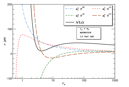
Figure 1: ${\mu_{R}}$ dependence of the LO and higher order corrections (FO) for LHC13, keeping $\mu_{F}=m_{\rm H}$ fixed.

In the FO results (Eq. RG improved Higgs boson production to N³LO in QCD), the dependence on $\mu_{R}$ enters through the evolution of $a_{s}(\mu_{R}^{2})$ as well as the perturbative corrections that are polynomials in $L_{R}$ of the order $k\leq n$ consistent with RG invariance. As $\mu_{R}$ decreases, the coupling constant as well as the magnitude of $L_{R}$ will increase, consequently, for $\mu_{R}$ much less than $m_{\rm H}$, the contributions of the kind $a_{s}^{n}\beta_{0}^{k}L_{R}^{k}$ can become large enough to make the $\mu_{R}$ dependent terms even negative. Moreover, at higher orders, the contribution of polynomial in $L_{R}$ need not be monotonic, instead it can change its sign with decreasing $\mu_{R}$ as seen in fig.1. With increase in $L_{R}$, the presence of the terms $(\beta_{0}a_{s}L_{R})^{k}$ makes the truncation of the perturbation series unreliable. The solution, proposed in this letter, resulting from RG improved resummation of those terms that spoil the perturbation series, shows an impressive improvement at every order. In fig.2, we show both the FO and the RESUM cross sections up to N³LO for LHC13 by varying $\mu_{R}$ in the range $[0.1m_{\rm H},10m_{\rm H}]$ and keeping $\mu_{F}=m_{\rm H}$ fixed. For $\mu_{R}<m_{\rm H}$, as discussed before, the large contributions from $L_{R}$ make the FO QCD corrections flip the sign and hence the cross sections take a downturn below certain $\mu_{R}$. This phenomenon can foremost be seen for cross section at higher orders, e.g., for $\mu_{F}=m_{\rm H}$ the N³LO cross section starts declining below $\mu_{R}=0.5m_{\rm H}$, followed by NNLO cross section at $\mu_{R}=0.2m_{\rm H}$ and so on. For $\mu_{F}=2m_{\rm H}$ also a similar pattern can be seen. For larger values of $\mu_{R}>m_{\rm H}$, however, $a_{s}(\mu_{R}^{2})$ falls down suppressing the logarithmic contributions and hence the cross sections will decrease monotonically. We have also plotted the RESUM cross sections at various orders in Fig. 2 as a function of $\mu_{R}$. We find that the predictions from the RESUM cross sections are more stable compared to the FO ones over a wide range of $\mu_{R}$ demonstrating the power and the reliability of resummation.

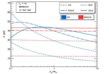
Figure 2: ${\mu_{R}}$ dependence of both the fixed order and resummed cross sections up to N³LO.

	LO	NLO	NNLO	N3LO
FO (%)	167.26	143.40	54.99	27.01
RESUM (%)	6.11	5.47	3.39	1.23

Table 1: Percentage of maximum uncertainty for $\mu_{R}$ variation in the range [$0.1m_{\rm H},10m_{\rm H}$] up to N³LO (see text).

In Table 1, we show the maximum percentage of uncertainty in the cross sections up to N³LO for $\mu_{R}$ variation in the range $[0.1m_{\rm H},10m_{\rm H}]$. Here, at N³LO, the $\mu_{R}$ uncertainty is maximum for $\mu_{R}$ between about $0.1m_{\rm H}$ and $0.5m_{\rm H}$ whereas at NNLO, the maximum uncertainty is for $\mu_{R}$ between about $0.2m_{\rm H}$ and $10m_{\rm H}$. We notice that the scale uncertainties in both FO and RESUM cross sections decrease with the order of the perturbation theory, as expected.

We also study the scale uncertainties of both the FO and RESUM cross sections up to N³LO as a function of the center of mass energy $\sqrt{s}$ of the incoming protons at the LHC and our results are given in fig.3. Here, we vary $\mu_{R}$ in the range $[0.1m_{\rm H},10m_{\rm H}]$ fixing $\mu_{F}=m_{\rm H}$. In general, the scale uncertainties in both FO and RESUM results are found to increase with $\sqrt{s}$ precisely because of the increase in gluon fluxes. Irrespective of the order of the perturbation theory, the RESUM results are found to decrease the scale uncertainties remarkably compared to the FO results. Here, at N³LO, the cross sections will increase from $\mu_{R}=0.1m_{\rm H}$ to about $\mu_{R}=0.5m_{\rm H}$ ( shown as solid lines in the Fig.3, the dashed line corresponds to the one at $\mu_{R}=10m_{\rm H}$) and then start decreasing with further $\mu_{R}$ variation. Also for $\mu_{R}>m_{\rm H}$, the N³LO cross section will decrease. Consequently for N³LO, the cross sections at the end points of the $\mu_{R}$ variation i.e. $0.1m_{\rm H}$ and $10m_{\rm H}$, will both be below the one at $\mu_{R}=m_{\rm H}$.

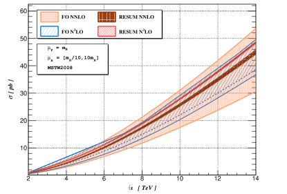
Figure 3: Dependence of scale uncertainties in both the fixed order and resummed cross sections on $\sqrt{s}$ (see text).

In conclusion, we have investigated the dependence of both the fixed order as well as the resummed predictions on the renormalization scale, using the recently available results on the Higgs boson production to N³LO in gluon fusion. For the resummed results, we systematically include all the RG accessible logarithms, $L_{R}$, to all orders in the perturbation theory. While the fixed order N³LO result shows impressive scale reduction for the canonical choice of the renormalization scale between $m_{\rm H}/2$ and 2 $m_{\rm H}$, there is still a significant dependence on the scale through these large logarithms which can spoil the behavior if the renormalization scale is varied further away from this range. On the other hand, the resummed results obtained in this letter show little dependence on the scale choice. For $\mu_{R}$ in the range $[0.1m_{\rm H},10m_{\rm H}]$, the RG improved cross sections bring the scale uncertainties from about $27$% down to about $1.5$% at N³LO level. This approach can also be used for other processes such as top pair production, multi-jet production etc.
Acknowledgments : We thank Nandadevi cluster computing facility at the Institute of Mathematical Sciences (IMSc) where the computation was carried out. GD thanks for the hospitality provided by IMSc where part of the work was done. GD also thanks P. Mathews for useful discussions and for his encouragement.

References

• (1) C. Anastasiou, C. Duhr, F. Dulat, F. Herzog and B. Mistlberger, arXiv:1503.06056 [hep-ph].
• (2) G. Aad et al. [ATLAS Collaboration], Phys. Lett. B 716, 1 (2012) ; S. Chatrchyan et al. [CMS Collaboration], Phys. Lett. B 716, 30 (2012).
• (3) H. M. Georgi, S. L. Glashow, M. E. Machacek, and D. V. Nanopoulos, Phys. Rev. Lett. 40 (1978) 692 ; A. Djouadi, M. Spira, and P. M. Zerwas, Phys. Lett. B 264 (1991) 440 ; S. Dawson, Nucl. Phys. B359 (1991) 283 ; M. Spira, A. Djouadi, D. Graudenz, and P. M. Zerwas, Nucl. Phys. B453 (1995) 17 ; S. Catani, D. de Florian and M. Grazzini, JHEP 0105 (2001) 025 ; R. V. Harlander and W. B. Kilgore, Phys. Rev. D 64 (2001) 013015 , Phys. Rev. Lett. 88 (2002) 201801 ; C. Anastasiou and K. Melnikov, Nucl. Phys. B646 (2002) 220 ; V. Ravindran, J. Smith, and W. L. van Neerven, Nucl. Phys. B665 (2003) 325.
• (4) S. Catani, D. de Florian, M. Grazzini, and P. Nason, JHEP 0307 (2003) 028.
• (5) U. Aglietti, R. Bonciani, G. Degrassi and A. Vicini, Phys. Lett. B 595 (2004) 432 ; S. Actis, G. Passarino, C. Sturm and S. Uccirati, Phys. Lett. B 670 (2008) 12 .
• (6) C. Anastasiou, C. Duhr, F. Dulat, E. Furlan, T. Gehrmann, F. Herzog and B. Mistlberger, Phys. Lett. B 737 (2014) 325 .
• (7) T. Ahmed, M. Mahakhud, N. Rana and V. Ravindran, Phys. Rev. Lett.  113 (2014) 11, 112002 ; T. Ahmed, M. K. Mandal, N. Rana and V. Ravindran, Phys. Rev. Lett.  113 (2014) 212003 ; S. Catani, L. Cieri, D. de Florian, G. Ferrera and M. Grazzini, Nucl. Phys. B 888 (2014) 75 ; T. Ahmed, N. Rana and V. Ravindran, JHEP 1410 (2014) 139 ; T. Ahmed, M. K. Mandal, N. Rana and V. Ravindran, JHEP 1502 (2015) 131 ; M. C. Kumar, M. K. Mandal and V. Ravindran, JHEP 1503 (2015) 037.
• (8) J. Baglio and A. Djouadi, JHEP 1010 (2010) 064 .
• (9) V. Ahrens, T. Becher, M. Neubert and L. L. Yang, Phys. Rev. D 79 (2009) 033013 .
• (10) V. Ahrens, T. Becher, M. Neubert and L. L. Yang, Eur. Phys. J. C 62 (2009) 333 .
• (11) M. R. Ahmady, F. A. Chishtie, V. Elias, A. H. Fariborz, N. Fattahi, D. G. C. McKeon, T. N. Sherry and T. G. Steele, Phys. Rev. D 66 (2002) 014010 .
• (12) S. Moch, J. A. M. Vermaseren and A. Vogt, Nucl. Phys. B 726 (2005) 317 .
• (13) A. D. Martin, W. J. Stirling, R. S. Thorne and G. Watt, Eur. Phys. J. C 63 (2009) 189 .
• (14) M. R. Whalley, D. Bourilkov and R. C. Group, hep-ph/0508110.