Quantum Critical Exponents for a Disordered Three-Dimensional Weyl Node

Abstract

Three-dimensional Dirac and Weyl semimetals exhibit a disorder-induced quantum phase transition between a semimetallic phase at weak disorder and a diffusive-metallic phase at strong disorder. Despite considerable effort, both numerically and analytically, the critical exponents $\nu$ and $z$ of this phase transition are not known precisely. Here we report a numerical calculation of the critical exponent $\nu=1.47\pm 0.03$ using a minimal single-Weyl node model and a finite-size scaling analysis of conductance. Our high-precision numerical value for $\nu$ is incompatible with previous numerical studies on tight-binding models and with one- and two-loop calculations in an $\epsilon$-expansion scheme. We further obtain $z=1.49\pm 0.02$ from the scaling of the conductivity with chemical potential.

Introduction.

Materials with an electronic bandstructure dispersing linearly from a Fermi point are among the driving themes in contemporary condensed matter physics Burkov2015 ; Cayssol2013 ; Wehling2014 . After the experimental verification of such a Dirac-type bandstructure in single-layer graphene Novoselov et al. (2005), the focus has now turned to three-dimensional materials. The compounds Na₃Bi and Cd₃As₂ have been confirmed as “Dirac semimetals” Liu et al. (2014); Neupane et al. (2014); Borisenko et al. (2014); Jeon et al. (2014); He et al. (2014). In materials that break either time- or space inversion symmetry, the twofold band degeneracy of Dirac semimetals is lifted and the resulting phase is termed Weyl semimetal. The non-centrosymmetric compounds TaAs and NbAs have recently proven experimentally to harbor such Weyl nodes in their bandstructures Lv et al. ; Xu et al. (2015); Xu2015b . Similar bandstructures have been achieved in a photonic crystal realization in Ref. Lu2015 .

Theoretical work accompanied and, in part, preceded the recent experiments. Beyond the single particle picture, Coulomb interactions were argued to be marginally irrelevant in the renormalization group (RG) sense due to the vanishing density of states at the Fermi point Goswami and Chakravarty (2011); Hosur2012 . Quenched disorder, however, inevitably present in realistic materials, is a much more subtle issue. Dating back to work from the 1980s Fradkin (1986, 1986), the presence of a disorder-induced quantum phase transition is by now firmly established analytically Goswami and Chakravarty (2011); Ominato and Koshino (2014); Syzranov et al. (2014, 2014) and numerically Kobayashi et al. (2014); Pixley et al. (2015); Pixley2015a ; Bera2015 ; Liu2015 ; Sbierski et al. (2014). In the weak-disorder phase, the random potential is irrelevant in an RG sense. Thus, for large system sizes and low temperatures, a weakly disordered system qualitatively behaves as a clean system with renormalized Fermi velocity. This leads to a number of experimentally important predictions for weak disorder, such as quadratically vanishing density of states Kobayashi et al. (2014); Syzranov et al. (2014) or pseudoballistic charge transport Sbierski et al. (2014) at the nodal point. In contrast, for strong disorder one finds a metallic phase with finite density of states at the Fermi energy and diffusive transport characteristics Sbierski et al. (2014); Altland and Bagrets (2015).

Signatures of the disorder-induced quantum criticality are expected in almost any experimentally relevant observable, from heat capacity to transport properties. Standard scaling theory Cardy (1996) predicts power-law dependences on disorder, chemical potential, or temperature in the vicinity of the critical point Kobayashi et al. (2014); Syzranov et al. (2014). The only input to this variety of predicted power laws is a pair of critical exponents characteristic of the universality class. Denoting the dimensionless disorder strength and chemical potential by $K$ and $\mu$, respectively, close to the critical point $K=K_{\rm c}$, $\mu=0$ the correlation length exponent $\nu$ and the dynamical critical exponent $z$ govern the relation between reduced disorder strength $k=|K-K_{\rm c}|/K_{\rm c}$ and the emerging correlation length $\zeta$ as $\zeta\propto k^{-\nu}$, and the relation between emergent energy- and length scales as $\varepsilon\propto\zeta^{-z}$. Although the critical point is located at zero chemical potential, predictions of scaling theory persist for small finite doping.

To date, the best analytical estimates for $\nu$ and $z$ for a single Weyl- or Dirac node follow from a Wilsonian momentum shell RG calculation in an $\epsilon$-expansion scheme around critical dimension two. The results of the one-loop calculation by Goswami and Chakravarty are $\nu=1$ and $z=1.5$ Goswami and Chakravarty (2011). The accuracy of the one-loop exponents was challenged by a calculation of two-loop diagrams by Roy and Das Sarma Roy and Sarma (2014), who found $\nu=1.14$ and $z=1.31$. On the other hand, there are instances where the $\epsilon$ expansion strategy is known to fail completely, the Anderson metal-insulator transition in three dimensions being a well known example Kramer and McKinnon (1993) — although the present transition is of a different type as it connects two non-insulating phases Pixley et al. (2015). Numerical results for the critical exponents obtained from tight-binding models harboring multiple Weyl- or Dirac nodes Kobayashi et al. (2014); Pixley et al. (2015); Pixley2015a ; Bera2015 ; Liu2015 are in reasonable agreement with the one-loop results above, albeit with large uncertainties in $\nu$, $z$ and $K_{\mathrm{c}}$.

Motivated by the lack of a firm theoretical prediction and in view of potential experiments, we performed a numerical calculation of the critical exponents in a single Weyl node using state of the art finite-size scaling for quantum transport properties. Our results, which we report in detail below, have significantly reduced uncertainties in comparison to the previously known estimates. Whereas our result for the dynamical critical exponent, $z=1.49\pm 0.02$, is consistent with the previous numerical calculations and with the one-loop calculation (but not with the two-loop calculation!), our value for the correlation length exponent, $\nu=1.47\pm 0.03$, deviates rather significantly.

Minimal model and numerical method.

The minimal model for the disorder induced quantum criticality is a single Weyl node with potential disorder,

$$H=\hbar v\boldsymbol{\sigma}\cdot\mathbf{k}+\mu+U(\mathbf{r}),$$ (1)

where $v$ is the Fermi velocity, $\boldsymbol{\sigma}$ denotes the vector of Pauli matrices, and $\mathbf{k}$ measures the Bloch wavevector relative to the nodal point. We connect the Weyl semimetal to two ideal leads, both modeled as Weyl nodes with $\mu$ taken to infinity and without the random potential $U$. The Weyl semimetal has dimension $0<x<L$ and $0<y,z<W$ in transport and transverse directions, respectively. To quantize transverse momenta $k_{y,z}$ we apply periodic or antiperiodic boundary conditions (PBC/APBC). An ultraviolet cutoff $\Lambda$ restricts the magnitude of transverse wavevector $|k_{y,z}|\leq\Lambda$ and $1/\Lambda$ sets the microscopic length scale. The random potential $U\left(\mathbf{r}\right)$ is assumed to have zero mean and Gaussian white noise fluctuations

$$\left\langle U(\mathbf{r})U(\mathbf{r}^{\prime})\right\rangle=\frac{K}{\Lambda}(\hbar v)^{2}\delta(\mathbf{r}-\mathbf{r}^{\prime}),$$ (2)

with $K$ the dimensionless disorder strength. The chemical potential $\mu$ has to vanish to reach the critical point, however, we will work with finite $\mu$ below to assess the dynamical critical exponent $z$.

We study the signatures of disorder-induced quantum criticality of Eq. (1) in a quantum transport framework at zero temperature, employing the numerical scattering matrix method of Ref. Sbierski et al. (2014), which is based on related studies of disordered Dirac fermions in two dimensions Bardarson et al. (2007); Adam et al. (2009). The conductance can be computed from the scattering matrix’s transmission block $t$ using the Landauer formula $G=\mathrm{tr}\,tt^{\dagger}$ and is measured in units of $e^{2}/h$ throughout.

Correlation length exponent $\nu$: Finite-size scaling of the conductance for $\mu=0$.

The standard method to assess the correlation length exponent $\nu$ is finite-size scaling Cardy (1996). To perform such an analysis, one needs to identify a dimensionless observable that assumes different values on the two sides of the (bulk) phase transition. In Ref. Sbierski et al. (2014) we showed numerically that the conductance $G$ fulfills these requirements. For large aspect ratio $r\equiv W/L\gg 1$ and in the thermodynamic limit $L\rightarrow\infty$, the conductance takes the values $G_{K=0}=r^{2}(\ln 2/2\pi)\simeq 0.11r^{2}$ in the pseudoballistic phase at disorder strength $K=0$ Baireuther2014 and $G_{K\to\infty}=\sigma r^{2}L\rightarrow\infty$ in the diffusive phase for $K>K_{\rm c}$ (with bulk conductivity $\sigma$) Sbierski et al. (2014). In the vicinity of the critical point $K=K_{\rm c}$, when the system dimensions $L$, $W$ are larger than all internal length scales other than the emerging correlation length $\zeta$, $G$ assumes a scaling form $G=G(L/\zeta,W/\zeta)$. Using $\zeta\propto k^{-\nu}$ and fixing the aspect ratio $r=W/L$, we arrive at $G=G_{r}(L^{1/\nu}k)$, with universal correlation length exponent $\nu$ and a scaling function $G_{r}$ that depends on $r$ and the boundary conditions.

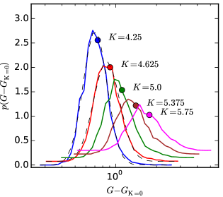
Numerically, the conductance $G$ is found to vary considerably for different disorder realizations, however with the restriction $G>G_{K=0}$ for every disorder realization. The histogram of $\delta G\equiv G-G_{K=0}$ is shown in Fig. 1 for the specific choice $L=2\pi/(\Lambda r)\times 11$, PBC. For weak disorder, $K\lesssim 5$, we find that the distribution of $\delta G$ can be well fitted by a log-normal distribution $p_{\rm LN}(\delta G)=e^{-(\ln\delta G-\mu_{\rm LN})^{2}/2\sigma_{\rm LN}^{2}}/\sigma_{LN}\delta G\sqrt{2\pi}$, with parameters $\mu_{\rm LN}$ and $\sigma_{\rm LN}$, see Fig. 1. A feature not captured by this fit is the tail of large but rare conductances, which are possibly related to rare region effects Nandkishore et al. (2014). As $G$ is not self-averaging (analogous to Anderson localization), we choose the median $m$ of the distribution as a scaling quantity, i.e., we search a scaling function $m=m_{r}(L^{1/\nu}k)$. The standard error of the median is calculated using the asymptotic variance formula $\sigma_{m}^{2}=1/4p(m)^{2}N$, where $N$ is the total number of disorder realizations and the unknown exact probability density $p$ is approximated by a smooth interpolation of the measured histogram. For further research, it would be desirable to understand the occurrence of the empirical log-normal conductance distribution.

Figure 1: (color online) Probability distribution of the difference $\delta G=G-G_{K=0}$ of the conductance with and without disorder potential. The aspect ratio $r=W/L=5$, periodic boundary conditions were applied in the transverse direction, and the sample length $L=(2\pi/\Lambda)\times 11/r$. The dimensionless disorder strength is indicated in the figure. The number of disorder realizations is 4000. Dots indicate the value of the median $m$, which is used as the scaling variable. Dashed lines show fits to a log-normal probability distribution. The data for $K>4.25$ is offset in vertical direction for clarity.

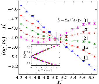
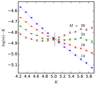
We compute $m$ for a range of disorder strengths $K$ and lengths $L$, for aspect ratios $r=5$ and $7$, and we also varied the boundary condition between periodic and anti-periodic. The data for $r=5$, PBC, is shown in Fig. 2, the other data sets can be found in the supplemental information, Ref. SI . At criticality, where $\zeta$ diverges, $m_{r}$ is independent of $L$ and the data traces in Fig. 2 cross in one point. In the supplemental information SI , we show the details of a least squares fit for $m_{r}\left(L^{1/\nu}k\right)$ for small $k$ to a polynomial of fourth order in $L^{1/\nu}k$ (solid lines). An excellent and stable fit was achieved even without including any irrelevant scaling variable that we took in leading order as $L^{y}$ with $y<0$. Taking into account the fitting results of all other parameter sets in a standard procedure (see SI ) we find $\nu=1.47\pm 0.03$. The conductance data for smaller aspect ratios $r\lesssim 3$ (data not shown) reveals a large irrelevant contribution to the scaling function that hindered a successful fit in terms of a simple low order polynomial.

In Ref. Sbierski et al. (2014) it was argued that the Fano factor $F$ (the ratio of shot-noise power and conductance) is an alternative quantity to distinguish the pseudoballistic from the diffusive phase. In the pseudoballistic phase one has $F(K<K_{\mathrm{c}})\simeq 0.574$ while in the diffusive phase $F(K>K_{\mathrm{c}})=1/3$. In the Supplemental Material we show that our result for $\nu$ is consistent with the value obtained from a finite-size scaling analysis using the Fano factor ($\nu=1.40\pm 0.05$). This method however suffers from an inferior quality of the data set, both in terms of error bars of the individual data points as well as in the range of system sizes available.

Figure 2: (color online) Scaling plot for the logarithm of the median $m$ of the distribution of $\delta G=G-G_{K=0}$ for a disordered Weyl node with $W/L=5$ and periodic transverse boundary conditions. For better visibility we plot $log(m)-K$ vs. $K$ on the vertical axis. The solid curves show the results of a least-squares fit to a scaling form $m=m_{r}(L^{1/\nu}k)$, expanded in a fourth order polynomial (for details, see SI ). The estimates for the most important fit parameters and their standard error are $K_{\rm c}=5.024\pm 0.004$, $\log(m_{\rm c})=0.12\pm 0.004$, $\nu=1.47\pm 0.02$. The quality of the fit is $\chi^{2}/N=0.93$. The sample lengths are indicated in the figure. The gray vertical line indicates the position of the estimated critical disorder strength. The inset shows a scaling collapse of the data in the main panel using the estimated values of $K_{\rm c}$ and $\nu$.

Dynamical critical exponent: Scaling of critical bulk conductivity.

We now turn to the dynamical critical exponent $z$ that connects the emergent length scale $\zeta$ and the corresponding energy scale $\varepsilon$ in the vicinity of the fixed point. In our transport geometry, a natural choice of a quantity that has a scaling involving the dynamical exponent $z$ is the bulk conductivity $\sigma$, which is also of immediate experimental relevance.

To connect the dynamical critical exponent to the conductivity, we again start with a scaling form around criticality Syzranov et al. (2014). Since the unit of $\sigma$ in three dimensions is inverse length, we find $\sigma\left(k,\mu\right)=\zeta^{-1}f(\mu/\varepsilon)$ with an unknown dimensionless scaling function $f$. We define a new scaling function $f\left(x\right)=x^{1/z}\tilde{f}\left(x^{-1}\right)$ in terms of which $\sigma\left(k,\mu\right)=\mu^{1/z}\tilde{f}\left(k^{z\nu}/\mu\right)$ . At $K=K_{\mathrm{c}}$, the ‘critical’ conductivity $\sigma_{\mathrm{c}}$ thus scales as

$$\sigma_{\mathrm{c}}\left(\mu\right)\propto\mu^{1/z}.$$ (3)

The scaling form (3) is valid with small corrections within an extended quantum critical region Syzranov et al. (2014) for finite $k$ when the argument of $\tilde{f}$ is sufficiently small, i.e. $k\ll k^{*}\left(\mu\right)\propto\mu^{1/(\nu z)}$. This allows us to numerically compute an estimate of $z$ in spite of the fact that the value of $K_{\rm c}$ is known only within error bars.

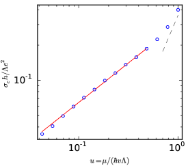
We compute $G(L)$ for fixed large $W$, PBC, a range of $\mu$ and for $K=5.0$, which is within the $K_{\rm c}$ confidence interval SI . We perform a disorder average over at least ten disorder realizations. Since transport in a Weyl node at finite $\mu$ is diffusive, we expect $G=\sigma W^{2}/L$, which is confirmed in the simulation. Finite size effects are irrelevant once $W,L$ are larger than the characteristic $\mu$-induced length scale $\propto\mu^{-1/z}$. We show $\sigma_{c}$ vs. $\mu$ for $K=K_{\rm c}$ in Fig. 3 (dots) and indeed observe a power law (solid line) for $\mu\lesssim\hbar v\Lambda$ with inverse exponent $z=1.49\pm 0.02$. For larger chemical potentials, $\mu$ comparable to the band edge $\hbar v\Lambda$, the scaling breaks down and from Drude transport theory we expect a crossover to $\sigma\propto\mu^{2}$, proportional to the density of states (dashed line).

Figure 3: Scaling of the conductivity $\sigma\left(K,\mu\right)$ for (near) critical disorder strengths $K=5.0$ (dots) with chemical potential $\mu$. The solid line is a power-law fit $\sigma\propto\mu^{1/z}$ to the data points, with $z=1.49\pm 0.02$. The dashed line indicates a $\sigma\propto\mu^{2}$ power law as expected from Drude transport theory when scaling breaks down. The sample width $W=(2\pi/\Lambda)\times 29$ and periodic boundary conditions were applied. For chemical potentials below the values shown in the figure a bulk conductivity could not be reliably obtained from the calculated conductance data.

Discussion.

We numerically studied the disorder-induced quantum phase transition in three-dimensional Dirac materials in terms of a minimal model, a single Weyl node with potential disorder. In contrast to the well-known Anderson metal-insulator transition, this disorder-induced phase transition for a single Weyl node is between two non-insulating phases. In addition to the correlation-length exponent $\nu$, it features a non-trivial dynamical critical exponent $z$, which has no counterpart in the standard metal-insulator transition.

Our high-precision results for the exponents $\nu$ and $z$ not only allow for a variety of quantitative predictions of experimentally observable power laws around criticality — such as the density-of-states exponent $\beta=\nu(3-z)$ for $K>K_{\rm c}$ Kobayashi et al. (2014) — but also improve on previously reported theoretical predictions. Our result $\nu=1.47\pm 0.03$ differs significantly from analytical results obtained from a one- or two-loop $\varepsilon$-expansion RG calculation ($\nu=1$, $1.14$, respectively Goswami and Chakravarty (2011); Roy and Sarma (2014)). The failure of the $\epsilon$-expansion calculation is reminiscent of the situation for the Anderson localization in three dimensions Kramer and McKinnon (1993), where $\nu=1.375$ in the symplectic class AsadaY2005 . Our estimate for the dynamical critical exponent is $z=1.49\pm 0.02$, in agreement with the one-loop RG calculation ($z=1.5$), but not with the two-loop prediction ($z=1.31$).

In principle, the model of Eq. (1), which has white-noise disorder and a sharp momentum cutoff, could be modified to include a more faithful representation of the microscopic disorder, albeit at an increased numerical cost. For example, Ref. Sbierski et al. (2014) employed a finite disorder correlation length that sets the microscopic length scale; the mode cutoff then can safely be taken to infinity. However, the difference between these two models is irrelevant in the RG sense and thus both models are in the same universality class. To see this, recall that a finite disorder correlation length is equivalent to a higher-order momentum dependence of the disorder-induced interaction vertex in the replicated disorder averaged action and is thus irrelevant Shankar (1994). On the other hand, the numerical value of $K_{\rm c}$ is non-universal and, thus, sensitive to the disorder model. In this context we note that a model with sharp momentum cut-off has also been used in Ref. Bardarson et al. (2007), where it was found to give the same results as a model with finite disorder correlation length. Moreover, in a realistic band structure the linear form of Eq. (1) is only an approximation. Quadratic corrections, however, are RG irrelevant and thus will not change the critical exponents Goswami and Chakravarty (2011).

Realistic Weyl and Dirac semimetals.

Realistic Weyl or Dirac semimetals have multiple Weyl nodes Nielsen and Ninomiya (1981), either separated in momentum space or distinguished by their transformation properties under point group symmetries. The same applies to numerical studies based on tight-binding models Kobayashi et al. (2014); Pixley et al. (2015); Pixley2015a ; Bera2015 ; Liu2015 , which confirmed the presence of a disorder-induced phase transition on the basis of density-of-states calculations. With multiple Weyl nodes, disorder might not only cause intra- but also inter-node scattering of quasiparticles. The latter process is not captured by our minimal model. Symmetries in more realistic models with multiple Weyl nodes may also be different from the minimal model: While our minimal model has an effective time-reversal symmetry mapping the single Weyl node onto itself, in realistic models, time-reversal or inversion symmetries can relate different nodes or be absent. Although the precise nature of disorder potentials in realistic three-dimensional Dirac materials is yet to be determined, there are plausible scenarios in which intra-node scattering dominates over inter-node scattering, a priori justifying the use of our minimal model. For example, in Weyl semimetals the ratio of scattering rates is controlled by the smoothness of the disorder potential and the separation of Weyl nodes in momentum space footnote_Dirac .

The applicability of the minimal model in the presence of sizeable inter-node scattering, i.e., the question whether or not the presence of some amount of inter-node scattering changes the universality class of the disorder-induced semimetal-metal transition, is an issue that has not been conclusively settled footnote_AL . Inter-node scattering is omitted in field-theoretical approaches Goswami and Chakravarty (2011); Syzranov et al. (2014). Empirical evidence that inter-node scattering does not affect the universality of the transition comes from Ref. Pixley2015a , which found a remarkable universality for three different disorder types in a tight-binding Dirac semimetal model, albeit with large error bars on the critical exponents.

If the assertion of a single universality class insensitive to inter- or intra-cone scattering (and the related symmetry differences) is correct, the observed critical exponents should match with those obtained in tight-binding models. However, such studies Kobayashi et al. (2014); Pixley et al. (2015); Pixley2015a ; Bera2015 ; Liu2015 yield a value for $\nu$ inconsistent with our result, for a typical example see Ref. Kobayashi et al. (2014) which finds $\nu=0.92\pm 0.13$ at $K>K_{\rm c}$ and $\nu=0.81\pm 0.21$ at $K<K_{\rm c}$. The value of the dynamical critical exponent $z=1.5\pm 0.1$ from Ref. Kobayashi et al. (2014) is in agreement with our result. Assuming that the type of scattering is indeed immaterial for critical exponents, we attribute the large difference with the tight-binding model exponent $\nu$ to difficulties in accurately estimating the critical disorder strength from density-of-states data. The uncertainty of $K_{\rm c}$ translates to a large uncertainty in the critical exponent $\nu$. In contrast, our very precise estimate of $K_{\rm c}$ was possible using the finite-size scaling method where $K_{\rm c}$ can be obtained from the unique crossing of the data in Fig. 2.

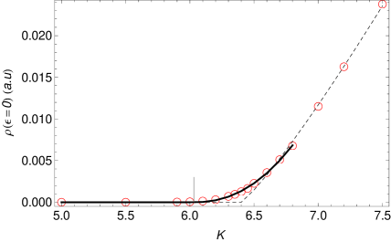
In the supplemental information SI , we exemplify this interpretation by revisiting the density of states data from Ref. Kobayashi et al. (2014) (cf. Fig. 3a) obtained at zero energy for a range of disorder values around the critical disorder strength. Using the critical exponent $\beta=2.22$ calculated with our estimates for $\nu$ and $z$ we are able to produce an excellent fit for the data points in the vicinity of the critical disorder strength, though we find a much smaller critical disorder strength than asserted in Ref. Kobayashi et al. (2014). Since the microscopic model in Ref. Kobayashi et al. (2014) and in this work are different, the values of the non-universal critical disorder strengths cannot be compared. Uncertainty in $K_{\rm c}$ does not cause comparable problems when determining the critical exponent $z$, because the large size of the critical region in the chemical potential–disorder parameter plane renders the extraction of $z$ much less sensitive to the uncertainty in $K_{\rm c}$. This is consistent with the mutual agreement between our estimate for $z$ and the value in Ref. Kobayashi et al. (2014).

Supplemental Material

Details of the finite-size scaling analysis.

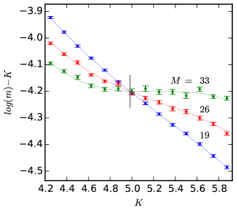
We here provide details of the finite-size scaling procedure, following Refs. Slevin and Ohtsuki (1999); Obuse et al. (2012, 2014, 2013). In addition to the data set presented in the main text — aspect ratio $r=5$ and periodic boundary conditions (PBC) —, we have obtained conductance distributions for antiperiodic boundary conditions (APBC) with $r=5$ and for aspect ratio $r=7$, PBC.

The sample width $W=L\cdot r$ is set to be $W=(2\pi/\Lambda)(M-1/2)$ for APBC and $W=(2\pi/\Lambda)M$ for PBC, with $M$ a positive integer. The transverse wavenumbers are $k_{y,z}=(2\pi/W)n_{y,z}$, with $n_{y,z}=-M,-M+1,\ldots,M$ for PBC and $n_{y,z}=-M+1/2,-M+3/2,\ldots,M-1/2$ for APBC. A summary of all data sets used in this work is given in Table 1.

For each data set, the median $m(K,M)$ of the conductance distribution is determined. We perform a least-squares fit to a polynomial of the form

$$m(K,M) = a_{0}(1+b_{01}L^{y}+\ldots+b_{0q_{0}}L^{yq_{0}})+a_{1}\cdot(L^{1/\nu}k)\cdot(1+b_{11}L^{y}+\ldots+b_{1q_{1}}L^{yq_{1}})$$

$$\mbox{}+\ldots+a_{p}\cdot(L^{1/\nu}k)^{p}\cdot(1+b_{11}L^{y}+...b_{1q_{p}}L^{yq_{p}})$$

for medians obtained at the same value of the aspect ratio $r$ and the same boundary conditions. Data points (i.e., medians of conductance distributions) and fits are shown in Fig. 2 of the main text for $r=5$ and PBC, and in Fig. 4 for $r=5$, APBC, and and $r=7$, PBC. The following algorithm for the fitting procedure is used: The order of the polynomials in Eq. (Details of the finite-size scaling analysis.) is increased by adding a new fit parameter $a_{i}$ or $b_{ij}$ if (i) the merit function $\chi^{2}/N\in[0,\infty]$ ($N$ is the number of data points) for the resulting fit is lowered by more than 2% compared to the previous fit and (ii) the error of any fitting parameter (as calculated from error propagation theory) does not exceed the parameter’s estimate in magnitude. Initial values for each fitting procedure are chosen randomly and the parameter estimates for the best fit out of a few hundred fitting trials is reported in Table 1 along with the error estimates and the value of $\chi^{2}/N$. A fit is acceptable if $\chi^{2}/N<1$, another measure is the ‘goodness of the fit’ $\mathcal{G}\in[0,1]$ where $\mathcal{G}=1$ indicates a perfect fit (for definitions of $\mathcal{G}$ and $\chi^{2}/N$ see, for example, Ref. Obuse et al. (2014)).

Ideally, fitting parameters should not strongly depend on the number of different values of $M$ within a data set. We successfully checked the stability of the fitting results by repeating the fitting procedure above for reduced data sets (deleting data points of the largest or smallest $M$ in the data set $r=5$, PBC), as indicated in Table 1. Finally, the estimate for $\nu$ is calculated as an average of the best fit estimates for $\nu$ for each data set whereas the total error bars are unions of error bars from each single data set (’practical-error-bar procedure’, see Ref. Obuse et al. (2013)).

$r=W/L$	B.C.	$M$	$N$	$\chi^{2}/N$	$\mathcal{G}$	$\nu$	$K_{\rm c}$	$log(m_{\mathrm{c}})=a_{0}$	$a_{1}\cdot 10^{1}$	$a_{2}\cdot 10^{2}$	$-a_{3}\cdot 10^{2}$	$-a_{4}\cdot 10^{3}$
5	PBC	$11,16,21,26,31$	70	0.93	0.4	$1.47\pm 0.02$	$5.024\pm 0.004$	$0.12\pm 0.004$	$5.0\pm 0.1$	$3.0\pm 0.3$	$1.3\pm 0.1$	$1.8\pm 0.9$
5	PBC	$16,21,26,31$	56	0.62	0.94	$1.46\pm 0.02$	$5.007\pm 0.007$	$0.102\pm 0.006$	$4.9\pm 0.2$	$3.3\pm 0.4$	$1.2\pm 0.1$	$2.6\pm 1.2$
5	PBC	$11,16,21,26$	56	0.84	0.55	$1.48\pm 0.02$	$5.036\pm 0.006$	$0.128\pm 0.004$	$5.0\pm 0.1$	$3.2\pm 0.4$	$1.4\pm 0.1$	$2.3\pm 1.3$
5	APBC	$14,19,24,29$	56	0.97	0.29	$1.47\pm 0.02$	$5.031\pm 0.005$	$0.169\pm 0.004$	$4.9\pm 0.1$	$2.8\pm 0.3$	$1.1\pm 0.1$	$1.7\pm 0.8$
7	PBC	$19,26,33$	42	0.64	0.87	$1.47\pm 0.03$	$4.983\pm 0.009$	$0.782\pm 0.007$	$4.8\pm 0.2$	$2.1\pm 0.2$	$1.5\pm 0.2$	-

Table 1: Details of the finite-size scaling procedure. The left part of the table specifies the data sets subject to a least squares fit with model (Details of the finite-size scaling analysis.) while the right part gives the fitting results. Numbers with $\pm$ are error bars (one standard deviation). The range of disorder strength for all data sets is $K=4.25,\,4.375,\,...\,,\,5.875$.

Figure 4: (color online) Scaling plots for the logarithm of the median $m$ of the distribution of the difference $\delta G=G-G_{K=0}$ of the two-terminal conductance with and without disorder potential, for a Weyl node with aspect ratio $r=W/L=5$ and antiperiodic boundarity conditions (left) and $r=7$ and periodic boundary conditions (right). For clarity, we plot $log(m)-K$ vs. $K$. The solid curves show the results of a least-squares fit to a scaling form $m=m_{r}\left(L^{1/\nu}k\right)$ expanded in a fourth ($r=5$) and third ($r=7$) order polynomial, respectively. The estimates for the most important fit parameters are given in Table 1. The gray vertical line indicates the position of the estimated critical disorder strength.

Comparison with finite-size scaling for Fano factor.

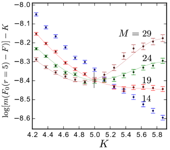
As discussed in the main text, besides the conductance, also the Fano factor can be expected to be a suitable observable for a finite-size scaling analysis. A scaling plot is shown in Fig. 5 and the details of the analysis (done as above for the conductance data) are reported in Table 2. Although the number of disorder realizations is comparable to the corresponding conductance data in Fig. 4 (left), for the Fano factor error bars are much larger. Moreover, while for conductance scaling data traces for system sizes $M=14,19,24,29$ all cross in a single point, the Fano factor data for $M=14$ does not cross with the traces of the larger system sizes, indicating that shot noise around criticality is controlled by larger emergent length scales than conductance. For the remaining system sizes, the analysis yields $\nu=1.40\pm 0.05$. Given the intrinsic difficulties for the Fano factor data discussed above we consider the error bar overlap with the conductance result $\nu=1.47\pm 0.03$ as a confirmation for consistency of the two finite-size scaling methods.

$W/L=r$	B.C.	$M$	$N$	$\chi^{2}/N$	$\mathcal{G}$	$\nu$	$K_{\rm c}$	$log(m_{\mathrm{c}})=a_{0}$	$a_{1}\cdot 10^{1}$	$a_{2}\cdot 10^{2}$	$a_{3}\cdot 10^{3}$	$a_{4}\cdot 10^{3}$
5	APBC	$19,24,29$	42	0.72	0.69	$1.40\pm 0.05$	$4.994\pm 0.015$	$-3.4\pm 0.01$	$4.3\pm 0.5$	$5.9\pm 1.5$	$-6\pm 2$	$-5\pm 3$

Table 2: Details of the finite-size scaling procedure for the Fano factor. The left part of the table specifies the data sets subject to a least squares fit with model (Details of the finite-size scaling analysis.) while the right part gives the fitting results. Numbers with $\pm$ are error bars (one standard deviation). The range of disorder strength is $K=4.25,\,4.375,\,...\,,\,5.875$.

Figure 5: (color online) Scaling plots for the logarithm of the median $m$ of the distribution of the difference $\delta F=F_{K=0}-F$ of the two-terminal Fano factor without and with disorder potential, for a Weyl node with aspect ratio $r=W/L=5$ and antiperiodic boundarity conditions. For clarity, we plot $log(m)-K$ vs. $K$. The solid curves show the results of a least-squares fit to a scaling form $m=m_{r}\left(L^{1/\nu}k\right)$ expanded in a fourth order polynomial. The data set for $M=14$ was not included in the analysis. The estimates for the most important fit parameters are given in Table 2. The gray vertical line indicates the position of the estimated critical disorder strength.

Comparison with density-of-states scaling for tight-binding model.

We revisit the results of a recent density-of-states simulation in a disordered Dirac semimetal from Ref. Kobayashi et al. (2014). The study is based on a large four-band tight-binding model tuned at the topological phase transition between a strong and weak topological insulator. If inter-node processes can be neglected, around criticality the density of states at zero energy should increase as $\rho(\epsilon=0)\propto(K-K_{\mathrm{c}})^{\beta}$ with $\beta=(3-z)\nu$. Using our estimate $\beta=2.2$, we successfully fit the data from from Ref. Kobayashi et al. (2014), (cf. Fig. 3a) in Fig. 6 (solid line), except for the three data points with largest disorder strength. In contrast, the emphasis in the interpretation of Ref. Kobayashi et al. (2014) was laid on data points for larger $K$, excluding the immediate vicinity of the critical point at $K=K_{\mathrm{c}}$. This leads to a larger estimate for $K_{\mathrm{c}}$ and a smaller estimate for $\beta$.

Figure 6: (color online) Bulk density of states of a disordered tight-binding model of a Dirac semimetal at zero energy as a function of disorder strength around criticality. The data (dots) is adapted from Ref. Kobayashi et al. (2014), Fig. 3a. The solid line is a fit to the scaling form $\rho(\epsilon=0)\propto(K-K_{\mathrm{c}})^{\beta}$ with $\beta=(3-z)\nu$ fixed to $2.22$ from our finite-size scaling analysis taking into account data points with $K<7$ only. The vertical gray line shows the corresponding estimate $K_{\mathrm{c}}=6.03$. The dashed line is a fit of the eight data points with the largest $K$ with setting $K_{\mathrm{c}}=6.4$ Kobayashi et al. (2014), the estimate for the exponent is $\beta=1.16$.

References

- (1) T. O. Wehling, A. M. Black-Schaffer, and A. V. Balatsky, Adv. Phys. 63, 1 (2014).
- (2) J. Cayssol, C. Rend. Phys. 14, 760 (2013); P. Hosur and X. Qi, ibid., 857.
- (3) A. Burkov, J. Phys.: Condens. Matter 27 113201 (2015).
- Novoselov et al. (2005) K. S. Novoselov, A. K. Geim, S. V. Morozov, D. Jiang, M. I. Katsnelson, I. V. Grigorieva, S. V. Dubonos, and A. A. Firsov, Nature 438, 197 (2005).
- Liu et al. (2014) Z. K. Liu, B. Zhou, Y. Zhang, Z. J. Wang, H. M. Weng, D. Prabhakaran, S.-K. Mo, Z. X. Shen, Z. Fang, X. Dai, Z. Hussain, and Y. L. Chen, Science 343, 864 (2014).
- Neupane et al. (2014) M. Neupane, S.-Y. Xu, R. Sankar, N. Alidoust, G. Bian, C. Liu, I. Belopolski, T.-R. Chang, H.-T. Jeng, H. Lin, A. Bansil, F. Chou, and M. Z. Hasan, Nat. Commun. 5, 3786 (2014).
- Borisenko et al. (2014) S. Borisenko, Q. Gibson, D. Evtushinsky, V. Zabolotnyy, B. Büchner, and R. J. Cava, Phys. Rev. Lett. 113, 027603 (2014).
- Jeon et al. (2014) S. Jeon, B. B. Zhou, A. Gyenis, B. E. Feldman, I. Kimchi, A. C. Potter, Q. D. Gibson, R. J. Cava, A. Vishwanath, and A. Yazdani, Nat. Mater. 13, 851 (2014).
- He et al. (2014) L. He, X. Hong, J. Dong, J. Pan, Z. Zhang, J. Zhang, and S. Li, Phys. Rev. Lett. 113, 246402 (2014).
- (10) B. Q. Lv, H. M. Weng, B. B. Fu, X. P. Wang, H. Miao, J. Ma, P. Richard, X. C. Huang, L. X. Zhao, G. F. Chen, Z. Fang, X. Dai, T. Qian, and H. Ding, Nat. Phys. 11, 724 (2015).
- Xu et al. (2015) S.-Y. Xu, I. Belopolski, N. Alidoust, M. Neupane, C. Zhang, R. Sankar, S.-M. Huang, C.-C. Lee, G. Chang, B. Wang, G. Bian, H. Zheng, D. S. Sanchez, F. Chou, H. Lin, S. Jia, M. Z. Hasan, Science 349, 613 (2015)
- (12) S.-Y. Xu, N. Alidoust, I. Belopolski, Z. Yuan, G. Bian, T.-R. Chang, H. Zheng, V. Strocov, D. S. Sanchez, G. Chang, C. Zhang, D. Mou, Y. Wu, L. Huang, C.-C. Lee, S.-M. Huang, B. Wang, A. Bansil, H.-T. Jeng, T. Neupert, A. Kaminski, H. Lin, S. Jia, M. Z. Hasan, Nat. Phys. 11, 748 (2015).
- (13) L. Lu, Z. Wang, D. Ye, L. Ran, L. Fu, J.-D. Joannopoulos, M. Soljačić, Science 349, 622 (2015)
- Goswami and Chakravarty (2011) P. Goswami, and S. Chakravarty, Phys. Rev. Lett. 107, 196803 (2011).
- (15) P. Hosur, S. A. Parameswaran, and A. Vishwanath, Phys. Rev. Lett. 108, 046602 (2012).
- Fradkin (1986) E. Fradkin, Phys. Rev. B 33, 3263 (1986).
- Fradkin (1986) E. Fradkin, Phys. Rev. B 33, 3257 (1986).
- Ominato and Koshino (2014) Y. Ominato and M. Koshino, Phys. Rev. B 89, 054202 (2014).
- Syzranov et al. (2014) S. V. Syzranov, L. Radzihovsky, and V. Gurarie, Phys. Rev. Lett. 114, 166601 (2015).
- Syzranov et al. (2014) S. V. Syzranov, V. Gurarie, and L. Radzihovsky, Phys. Rev. B 91, 035133 (2015).
- Sbierski et al. (2014) B. Sbierski, G. Pohl, E. J. Bergholtz, and P. W. Brouwer, Phys. Rev. Lett. 113, 026602 (2014).
- Kobayashi et al. (2014) K. Kobayashi, T. Ohtsuki, K.-I. Imura, and I. F. Herbut, Phys. Rev. Lett. 112, 016402 (2014).
- Pixley et al. (2015) J. H. Pixley, P. Goswami, and S. Das Sarma, Phys. Rev. Lett. 115, 076601 (2015).
- (24) J. Pixley, P. Goswami, S. Das Sarma, arXiv1505.07938v1.
- (25) S. Bera, J. D. Sau, and B. Roy, arXiv1507.07551v1.
- (26) S. Liu, T. Ohtsuki, and R. Shindou, arXiv1507.02381v1.
- Altland and Bagrets (2015) A. Altland and D. Bagrets, Phys. Rev. Lett. 114, 257201 (2015).
- Cardy (1996) J. Cardy, Scaling and Renormalization in Statistical Physics (Cambridge University Press, Cambridge, England, 1996).
- Roy and Sarma (2014) B. Roy and S. Das Sarma, Phys. Rev. B 90, 241112(R) (2014).
- Kramer and McKinnon (1993) B. Kramer and A. McKinnon, Rep. Prog. Phys. 56, 1469 (1993).
- Bardarson et al. (2007) J. H. Bardarson, J. Tworzydlo, P. W. Brouwer, and C. W. J. Beenakker, Phys. Rev. Lett. 99, 106801 (2007).
- Adam et al. (2009) S. Adam, P. W. Brouwer, and S. Das Sarma, Phys. Rev. B 79, 201404 (2009).
- (33) P. Baireuther, J. M. Edge, I. C. Fulga, C. W. J. Beenakker, and J. Tworzydlo, Phys. Rev. B 89, 035410 (2014).
- Nandkishore et al. (2014) R. Nandkishore, D. Huse, and S. Sondhi, Phys. Rev. B 89, 245110 (2014).
- (35) See supplemental information.
- (36) Y. Asada, K. Slevin, and T. Ohtsuki, J. Phys. Soc. Japan 74, 238 (2005).
- Shankar (1994) R. Shankar, Rev. Mod. Phys. 66, 129 (1994).
- Nielsen and Ninomiya (1981) H. Nielsen and M. Ninomiya, Nucl. Phys. B185, 20 (1981).
- (39) For disordered Dirac semimetals where Weyl nodes coincide, spatial symmetries of the specific model can suppress inter-node scattering.
- (40) Inter-node scattering, if strong enough, leads to a standard Anderson localization transition for strong disorder Pixley et al. (2015), which can be regarded as a competing physical scenario.
- Slevin and Ohtsuki (1999) K. Slevin and T. Ohtsuki, Phys. Rev. Lett. 82, 382 (1999).
- Obuse et al. (2012) H. Obuse, I. A. Gruzberg, and F. Evers, Phys. Rev. Lett. 109, 206804 (2012)
- Obuse et al. (2014) H. Obuse, S. Ryu, A. Furusaki, and C. Mudry, Phys. Rev. B 89, 155315 (2014).
- Obuse et al. (2013) H. Obuse, S. Bera, A. W. W. Ludwig, I. A. Gruzberg, and F. Evers, Europhys. Lett. 104, 27014 (2013).