Abstract

Two-photon correlations in the thermal radiation field of a double-star system are studied. It is investigated how the differential Hanbury Brown and Twiss (HBT) approach can be used in order to determine orbital parameters of a binary star.

1 Introduction

Hanbury Brown and Twiss have discovered the remarkable fact that photons, emitted by some thermal light-source, tend to arrive at distant detectors in correlated pairs [1, 2]. As recognized by Hanbury Brown and Twiss, this HBT effect of photon correlation allows to determine the angular size of the thermal light-source. Soon afterwards, momentum-correlations among two pions created in heavy-ion collisions have been measured by Goldhaber et al. [3], which are a model-independent possibility in order to obtain information about the spatial size and the time-evolution of the hadronic fireball. Some typical two-pion correlation functions measured by experiments at CERN-SPS or at AGS-Brookhaven are shown in [4] and [5], respectively. Ever since, the HBT approach was used extensively for the study of relativistic heavy-ion reactions [6]; for a historical review see [7]. Meanwhile, the method was extended not only to detect the size of the source of emission, but also the speed of radial expansion [8], the rotational motion [9] and the turbulence [10] of the emitting source, also by means of the differential HBT method [11, 12, 13].

In the original work of Hanbury Brown and Twiss the HBT effect has been exploited in order to determine the spatial size of stars. Here, in our investigation we will revisit that astronomical problem and apply these new approaches to astrophysical situations with the main focus on binary systems. Accordingly, each companion of a double star is considered to be an individual thermal source of light and the photons of these stars are HBT correlated. Using this assumption, we will examine the possible applicability of the differential HBT method to determine some orbital parameter of a binary system: the semi-major axis $A$, orbital period $\mathcal{T}$, and orbital speed of the both components $\mbox{\boldmath$v$}_{A},\mbox{\boldmath$v$}_{B}$; see Fig. 1.

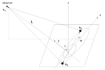
Figure 1: The orbit of a binary system is defined by seven orbital elements: distance $L$ between the center-of-mass of the binary star and the observer, semi-major axis $x$, inclination $0\leq i\leq\pi$, eccentricity $0\leq e<1$, eccentric anomaly $0\leq E\leq 2\pi$, periapsis $0\leq\omega\leq\pi$ and mass ratio $M_{1}/M_{2}$. Other familiar elements (e.g. orbital period $\mathcal{T}$ or orbital speed $\mbox{\boldmath$v$}_{1},\mbox{\boldmath$v$}_{2}$) can be deduced from these seven orbital elements. The elements $x$, $e$, and $M_{A}/M_{B}$ uniquely determine the shape of the both ellipses, while $i$ and $\omega$ determine the orientation of the orbital plane (here the $[x,y]$-plane), and a parameter $E$ determines the actual position of both components of the binary, ${\cal 1}$ and ${\cal 2}$. In case of a symmetric system where $M=M_{1}=M_{2}$ and $\mbox{\boldmath$r$}_{o}\equiv\mbox{\boldmath$r$}_{1}=-\mbox{\boldmath$r$}_{2}$, an idealized, circular orbit may be possible.

At the moment being, there are about $10^{5}$ binary systems (resolved, astrometric, eclipsing, spectroscopic) are known, according to the Washington Double Star Catalog [14]. However, only for a small part of all these binaries the complete set of all seven orbital elements have been determined so far. Consequently, the reason for our investigation is twofold: (i) The suggested approach could demonstrate the presence of the HBT effect in binary systems. (ii) Such an approach could allow for determining orbital parameter independently from standard astrophysical or astrometric approaches.

The paper is organized as follows: In Section 2 the HBT effect is reviewed for basic understanding, both in terms of classical electrodynamics and quantum electrodynamics. In Section 3 it is discussed how the advanced HBT approach used in heavy-ion physics has to be modified for the case of astrophysics. The emission function as essential element of the two-photon correlation function is determined in Section 4. Using this modified approach, the two-photon correlation function for a binary system is determined in Section 5. In Section 6 the case of one thermal light-source (one star) is considered, while the case of two thermal light-sources (binary star) is discussed in Section 7. A summary and outlook is given in Section 8.

Throughout the article, we use Heaviside-Lorentz units: $\epsilon_{0}=\mu_{0}=c=\hbar=1$, and for the Boltzmann constant $k_{B}=1$. Furthermore, the astronomical unit is denoted by $1\,{\rm a.u.}=1.49\times 10^{11}\,m$.

2 HBT effect

In 1954, Hanbury Brown and Twiss [15] have realized the idea of an intensity interferometer for classical electromagnetic radiation in the radio-band. Such intensity interferometry compares intensities of the incoming radiation field rather than amplitudes at different detection points. Originally, the basic idea was that intensity-measurements are able to improve the angular resolution of radiation-sources and do not account for the phase of the electromagnetic fields, hence are insensitive to phase shifts caused by atmospheric scintillations. They have first tested their intensity interferometer by determining the known angular size of the Sun, and later they succeeded in determining the angular size of the radio sources Cassiopaia A and Cygnus A [15].

In a first laboratory desk experiment, Hanbury Brown and Twiss have extended their new technology into the optical range of electromagnetic spectrum. They have used a light beam from a mercury vapor lamp, which is actually a thermal light source, and were able to detect second-order correlations among photons [1], being the discovery of a new physical effect. Afterwards, Hanbury Brown and Twiss succeeded with their technique in determining the angular size of the star Sirius by detecting photon correlations in the optical region [2].

While the correlation of radio waves is an effect which can fully be explained by classical electrodynamics, the correlation of photons in the HBT experiment initiated a heated debate about the concept of the photon at that time. Later, Glauber succeeded with a comprehensive theoretical explanation of the HBT effect in a series of articles [16, 17, 18]. Especially, Glauber (i) introduced the concept of higher-coherence in quantum electrodynamics [16], (ii) determined the explicit quantumfield-theoretical expression for coherent states (Glauber states) [17], (iii) determined the general expression for the density operator for coherent and incoherent states [18], and (iv) has shown that the HBT effect does not happen for Laser light sources (described by Glauber states), but occurs for extended thermal light sources (described by incoherent states) [18]. These articles were the birth of a new branch of science, the Quantum optics, for which he awarded the Physics Nobel Prize in 2005.

In general, in HBT measurements one records photons of a thermal light source by two detectors: detector A is located at $\mbox{\boldmath$x$}_{A}$ and detects incomming photons at time $t_{A}$, while detector B is located at $\mbox{\boldmath$x$}_{B}$ and detects incomming photons at time $t_{B}$. The spatial distance between both detectors is $d_{AB}=\left|\mbox{\boldmath$x$}_{A}-\mbox{\boldmath$x$}_{B}\right|$. Depending on the concrete experiment under consideration, two specific cases have to be distinguished: correlation measurement in space ($t_{A}=t_{B}$ and $\mbox{\boldmath$x$}_{A}\neq\mbox{\boldmath$x$}_{B}$) and correlation measurement in time ($t_{A}\neq t_{B}$ and $\mbox{\boldmath$x$}_{A}=\mbox{\boldmath$x$}_{B}$). In our investigation, correlation measurements in space are relevant, that means the incoming photons are recorded at the same time, $t_{A}=t_{B}$, while the distance $d_{AB}$ between both detectors is varied. In this way one can determine second-order correlations (HBT effect) of incoming photons, which are used to determine some physical parameters of the thermal light-source. Fundamental aspects of the HBT effect will be demonstrated by means of an elementary model for the thermal radiation.

2.1 HBT effect in terms of classical electrodynamics

In order to describe the HBT effect it is useful to subdivide the surface of a star with stellar radius $R$ into pointlike regions, each of which is considered as an emitter of spherical waves of thermal light, i.e. pointlike sources of black-body radiation. The entire radiation field of the star would finally been obtained by a summation over all of these pointlike regions over the whole surface of the star.

For the description of spherical waves it is advantageous to introduce spherical coordinates $\mbox{\boldmath$x$}=\left(x,y,z\right)\longrightarrow\mbox{\boldmath$r$}=\left(r,\theta,\phi\right)$, i.e. $x=r\,\cos\theta\,\cos\phi\,,\,y=r\,\cos\theta\,\sin\phi\,,\,z=r\,\cos\theta$. Here the origin of coordinate system is, first of all, assumed to be located at the center of a pointlike radiation source, hence $r=\left|\mbox{\boldmath$x$}\right|$ being the distance between the pointlike region of emission and some point with spatial coordinate $\mbox{\boldmath$x$}\leftrightarrow\mbox{\boldmath$r$}$ (later it will be the detector’s position). In general, the radiative part of electric field at sufficiently far distances from a localized radiation-source, defined by the wave-zone $k\,r\gg 1$ (wave-number $k$ is related to wavelength $\lambda$ in virtue of $k=2\,\pi/\lambda$), is given by the following multipole-expansion for one individual frequency $\omega_{k}=k$ [19]:

$$\mbox{\boldmath$E$}\left(\mbox{\boldmath$r$},t\right) = i\,\frac{{\rm e}^{i\left(k\,r-\omega_{k}\,t\right)}}{k\,r}\sum\limits_{l=1}^{\infty}\sum\limits_{m=-l}^{l}\alpha_{lm}\;\mbox{\boldmath$g$}_{lm}\left(\theta,\phi\right)+c.c.\,,$$ (1)

where we have assumed that the radiation source has no magnetic moments; $c.c.$ stands for complex-conjugate and $l\geq 1$ because there is no monopole radiation. Here, $\mbox{\boldmath$g$}_{lm}=\left(-i\right)^{l}\,\mbox{\boldmath$n$}\times\mbox{\boldmath$X$}_{lm}$ with the unit direction $\mbox{\boldmath$n$}=\mbox{\boldmath$r$}/r$ and the vector spherical harmonics $\mbox{\boldmath$X$}_{lm}=\mbox{\boldmath$l$}\,Y_{lm}/\sqrt{l\left(l+1\right)}$, the orbital angular-momentum operator is $\mbox{\boldmath$l$}=\mbox{\boldmath$r$}\times\mbox{\boldmath$\nabla$}$, and the spherical harmonics are $Y_{lm}$. The eigenvalues of the spherical harmonics are $\mbox{\boldmath$l$}^{2}\,Y_{lm}=l\left(l+1\right)Y_{lm}$ and $\mbox{\boldmath$l$}_{z}\,Y_{lm}=m\,Y_{lm}$. The electric multipole-coefficients are complex-valued numbers, $\alpha_{lm}=\left|\alpha_{lm}\right|\,{\rm e}^{i\,\varphi_{k}}$ with phase $\varphi_{k}$ .

In order to get an idea about the magnitude of wave-number k, we recall that a star is an almost ideal black body radiator, that means the wavelength of maximal intensity of a star is determined by Wien’s law of displacement, which states that the wavelength $\lambda_{\rm max}$ of maximal intensity of a star with surface temperature $T$ is given by $\lambda_{\rm max}=2.9\times 10^{-3}\,{\rm meter}\,{\rm Kelvin}/T$. The corresponding wave-vector $k_{\rm max}=2\,\pi/\lambda_{\rm max}$. For instance, Sirius has a surface temperature of about $9900\,{\rm K}$ and we obtain $\lambda_{\rm max}=2.92\times 10^{-7}\,{\rm meter}$ and $k_{\rm max}=2.15\times 10^{7}\,{\rm meter}^{-1}$. Therefore, it would be meaningful to determine the HBT effect with photo-detectors which are sensitive in the vicinity around $k_{\rm max}$.

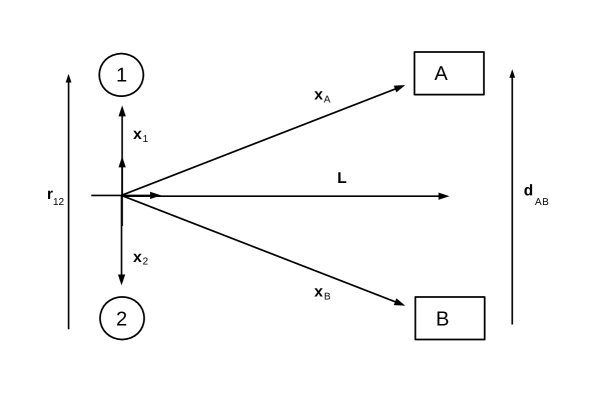
Figure 2: Two pointlike regions at $\mbox{\boldmath$x$}_{1}$ and $\mbox{\boldmath$x$}_{2}$ of the extended light source and two detectors located at $\mbox{\boldmath$x$}_{A}$ and $\mbox{\boldmath$x$}_{B}$. The vectors are defined by $\mbox{\boldmath$r$}_{12}=\mbox{\boldmath$x$}_{1}-\mbox{\boldmath$x$}_{2}$, $\mbox{\boldmath$d$}_{AB}=\mbox{\boldmath$x$}_{A}-\mbox{\boldmath$x$}_{B}$ and $\displaystyle\mbox{\boldmath$L$}=\frac{\mbox{\boldmath$x$}_{A}+\mbox{\boldmath$x$}_{B}}{2}$. Note that $\displaystyle\mbox{\boldmath$x$}_{A}=\mbox{\boldmath$L$}+\frac{\mbox{\boldmath$d$}_{AB}}{2}$ and $\displaystyle\mbox{\boldmath$x$}_{B}=\mbox{\boldmath$L$}-\frac{\mbox{\boldmath$d$}_{AB}}{2}$.

To simplify the notation, we assume the photo-detectors to be sensitive only for incoming light rays which are polarized in an arbitrary but fixed unit-direction $e$, thus we consider the vector-component of the electric field in this direction: ${\cal E}\left(\mbox{\boldmath$r$},t\right)=\mbox{\boldmath$e$}\cdot\mbox{\boldmath$E$}\left(\mbox{\boldmath$r$},t\right)$ [16], and we introduce the notation ${\it g}_{lm}=\mbox{\boldmath$e$}\cdot\mbox{\boldmath$g$}_{lm}$. Actually, the radiation distribution caused by a superposition of incoherent multipoles in the pointlike radiation-source is isotropic [19], hence independent of $m$. However, in HBT experiments one measures individual photons, which in the classical electrodynamics correspond to one single radiation-mode of the electric radiation-field in (1), given by:

$${\cal E}_{lm}\left(\mbox{\boldmath$r$},t\right) = i\,\frac{{\rm e}^{i\left(k\,r-\omega_{k}\,t\right)}}{k\,r}\alpha_{lm}\;{\it g}_{\,lm}\left(\theta,\phi\right)+c.c.\,.$$ (2)

For HBT effect, it is sufficient to consider the most simple case of two specific spherical-wave modes: one mode $l_{1}m_{1}$ originates from the pointlike region at $\mbox{\boldmath$x$}_{1}$ of the star’s surface, while another mode $l_{2}m_{2}$ originates from the pointlike region at $\mbox{\boldmath$x$}_{2}$ of the star’s surface. The collective electric field at detector position $\mbox{\boldmath$x$}_{A}$ and at time $t$ is then given by a superposition of these waves, cf. Fig. 2:

$${\cal E}\left(\mbox{\boldmath$x$}_{1},\mbox{\boldmath$x$}_{2},\mbox{\boldmath$x$}_{A},t\right) = {\cal E}_{l_{1}m_{1}}\left(\mbox{\boldmath$x$}_{1},\mbox{\boldmath$x$}_{A},t\right)+{\cal E}_{l_{2}m_{2}}\left(\mbox{\boldmath$x$}_{2},\mbox{\boldmath$x$}_{A},t\right).$$ (3)

Using the relation for a spherical wave-mode originating at $\mbox{\boldmath$x$}_{1}$ towards detector at $\mbox{\boldmath$x$}_{A}$ with momentum $\displaystyle\mbox{\boldmath$k$}_{1A}=k_{1}\frac{\mbox{\boldmath$x$}_{A}-\mbox{\boldmath$x$}_{1}}{\left|\mbox{\boldmath$x$}_{A}-\mbox{\boldmath$x$}_{1}\right|}$, and another spherical wave-mode originating at $\mbox{\boldmath$x$}_{2}$ towards detector at $\mbox{\boldmath$x$}_{A}$ with momentum $\displaystyle\mbox{\boldmath$k$}_{2A}=k_{2}\frac{\mbox{\boldmath$x$}_{A}-\mbox{\boldmath$x$}_{2}}{\left|\mbox{\boldmath$x$}_{A}-\mbox{\boldmath$x$}_{2}\right|}$, the scalar product takes the form

$$\mbox{\boldmath$k$}_{1A}\cdot\left(\mbox{\boldmath$x$}_{A}-\mbox{\boldmath$x$}_{1}\right) = k_{1}\left|\mbox{\boldmath$x$}_{A}-\mbox{\boldmath$x$}_{1}\right|\,,$$ (4)

$$\mbox{\boldmath$k$}_{2A}\cdot\left(\mbox{\boldmath$x$}_{A}-\mbox{\boldmath$x$}_{2}\right) = k_{2}\left|\mbox{\boldmath$x$}_{A}-\mbox{\boldmath$x$}_{2}\right|\,,$$ (5)

where the two electromagnetic spherical-waves, originating from region $\mbox{\boldmath$x$}_{1}$ and $\mbox{\boldmath$x$}_{2}$, are given by

$${\cal E}_{l_{1}m_{1}}\left(\mbox{\boldmath$x$}_{1},\mbox{\boldmath$x$}_{A},t\right) = i\,\left|\alpha_{l_{1}m_{1}}\right|\,{\it g}_{\,l_{1}m_{1}}\,\frac{{\rm exp}\left[i\left(k_{1}\,\left|\mbox{\boldmath$x$}_{A}-\mbox{\boldmath$x$}_{1}\right|-\omega_{k_{1}}\,t+\varphi_{k_{1}}\right)\right]}{k_{1}\;\left|\mbox{\boldmath$x$}_{A}-\mbox{\boldmath$x$}_{1}\right|}+c.c.\,,$$ (6)

$${\cal E}_{l_{2}m_{2}}\left(\mbox{\boldmath$x$}_{2},\mbox{\boldmath$x$}_{A},t\right) = i\,\left|\alpha_{l_{2}m_{2}}\right|\,{\it g}_{\,l_{2}m_{2}}\,\frac{{\rm exp}\left[i\left(k_{2}\,\left|\mbox{\boldmath$x$}_{A}-\mbox{\boldmath$x$}_{2}\right|-\omega_{k_{2}}\,t+\varphi_{k_{2}}\right)\right]}{k_{2}\;\left|\mbox{\boldmath$x$}_{A}-\mbox{\boldmath$x$}_{2}\right|}+c.c.\,,$$ (7)

where the phases are written explicitly. The electric field at detector B is obtained in a very same way, where $\mbox{\boldmath$x$}_{A}$ is simply replaced by $\mbox{\boldmath$x$}_{B}$. The correlation function of second-order, for these two spherical-waves is defined by

$$C\left(\mbox{\boldmath$x$}_{1},\mbox{\boldmath$x$}_{2},\mbox{\boldmath$x$}_{A},\mbox{\boldmath$x$}_{B}\right) = \frac{\langle I\left(\mbox{\boldmath$x$}_{1},\mbox{\boldmath$x$}_{2},\mbox{\boldmath$x$}_{A},t\right)\,I\left(\mbox{\boldmath$x$}_{1},\mbox{\boldmath$x$}_{2},\mbox{\boldmath$x$}_{B},t\right)\rangle}{\langle I\left(\mbox{\boldmath$x$}_{1},\mbox{\boldmath$x$}_{2},\mbox{\boldmath$x$}_{A},t\right)\rangle\,\langle I\left(\mbox{\boldmath$x$}_{1},\mbox{\boldmath$x$}_{2},\mbox{\boldmath$x$}_{B},t\right)\rangle}\,,$$ (8)

where the intensities $I\left(\mbox{\boldmath$x$}_{A},t\right)$ and $I\left(\mbox{\boldmath$x$}_{B},t\right)$ are defined as square of the absolute value of electric field and are measured by two intensity detectors located at $\mbox{\boldmath$x$}_{A}$ and $\mbox{\boldmath$x$}_{B}$,

$$I\left(\mbox{\boldmath$x$}_{1},\mbox{\boldmath$x$}_{2},\mbox{\boldmath$x$}_{A},t\right) = {\cal E}^{\ast}\left(\mbox{\boldmath$x$}_{1},\mbox{\boldmath$x$}_{2},\mbox{\boldmath$x$}_{A},t\right)\;{\cal E}\left(\mbox{\boldmath$x$}_{1},\mbox{\boldmath$x$}_{2},\mbox{\boldmath$x$}_{A},t\right)\,,$$ (9)

$$I\left(\mbox{\boldmath$x$}_{1},\mbox{\boldmath$x$}_{2},\mbox{\boldmath$x$}_{B},t\right) = {\cal E}^{\ast}\left(\mbox{\boldmath$x$}_{1},\mbox{\boldmath$x$}_{2},\mbox{\boldmath$x$}_{B},t\right)\;{\cal E}\left(\mbox{\boldmath$x$}_{1},\mbox{\boldmath$x$}_{2},\mbox{\boldmath$x$}_{B},t\right).$$ (10)

Thermal radiation fields are characterized by the fact that the amplitudes $\alpha_{lm}$ fluctuate independently of one another, that means their phases $\varphi_{k}$ are randomly distributed as well as their absolute values $\left|\alpha_{lm}\right|$. Accordingly, the thermodynamical average of a function ${\cal O}$ in (8) implies, first of all, an average over the phases and afterwards an average over the absolute values of the amplitudes. The average over the phases resembles the thermal average procedure originally introduced by the Einstein-Hopf model [20], and is given by:

$$\langle{\cal O}\rangle = \frac{1}{2\pi}\int\limits_{0}^{2\pi}{\cal O}\left(\varphi\right)\;d\varphi\,.$$ (11)

By using (3), (9) and (10), and performing an average according to (11) one obtains for the correlation function of second-order for two spherical-waves with equal frequencies $\omega_{k_{1}}=\omega_{k_{2}}$ the following expression:

$$C\left(\mbox{\boldmath$x$}_{1},\mbox{\boldmath$x$}_{2},\mbox{\boldmath$x$}_{A},\mbox{\boldmath$x$}_{B}\right)$$

$$=1+2\,\frac{\left|\alpha_{l_{1}m_{1}}\right|^{2}\,\left|\alpha_{l_{2}m_{2}}\right|^{2}}{\left(\left|\alpha_{l_{1}m_{1}}\right|^{2}+\left|\alpha_{l_{2}m_{2}}\right|^{2}\right)^{2}}\,\cos\bigg{[}k\left(\left|\mbox{\boldmath$x$}_{1}-\mbox{\boldmath$x$}_{A}\right|+\left|\mbox{\boldmath$x$}_{2}-\mbox{\boldmath$x$}_{B}\right|-\left|\mbox{\boldmath$x$}_{2}-\mbox{\boldmath$x$}_{A}\right|-\left|\mbox{\boldmath$x$}_{1}-\mbox{\boldmath$x$}_{B}\right|\right)\bigg{]}\,.$$

(12)

As stated above, we also have to perform a thermal average over the absolute values of the amplitudes in (12), and one easily obtains: the relations: $\langle\left|\alpha_{l_{1}m_{1}}\right|^{2}\rangle_{\rm th}=\langle\left|\alpha_{l_{2}m_{2}}\right|^{2}\rangle_{\rm th}$ and $\langle\left|\alpha_{l_{1}m_{1}}\right|^{2}\;\left|\alpha_{l_{2}m_{2}}\right|^{2}\rangle_{\rm th}=2\,\langle\left|\alpha_{l_{1}m_{1}}\right|^{2}\rangle^{2}_{\rm th}$. Then, the correlator in (12) finally yields [21]:

$$C\left(\mbox{\boldmath$x$}_{1},\mbox{\boldmath$x$}_{2},\mbox{\boldmath$x$}_{A},\mbox{\boldmath$x$}_{B}\right) = 1+\cos\bigg{[}k\left(\left|\mbox{\boldmath$x$}_{1}-\mbox{\boldmath$x$}_{A}\right|+\left|\mbox{\boldmath$x$}_{2}-\mbox{\boldmath$x$}_{B}\right|-\left|\mbox{\boldmath$x$}_{2}-\mbox{\boldmath$x$}_{A}\right|-\left|\mbox{\boldmath$x$}_{1}-\mbox{\boldmath$x$}_{B}\right|\right)\bigg{]}\,.$$

There are two important limits for the correlation function in (LABEL:Introduction_26), namely the case of stars and the case of heavy-ion collisions, cf. Refs. [22, 23]. Both limiting cases we shall consider in more detail.

2.1.1 Correlation function in the limit of stars

In case of a star we have the following limits: $L\gg r_{12}\gg d_{AB}$, where $L$ is the distance between star and detectors, $r_{12}$ is the distance among two pointlike regions on the star’s surface, and $d_{AB}$ is the distance between both detectors, see Fig.2. In these limits, the argument of the cosine-function in (LABEL:Introduction_26) can considerably been simplified and we obtain for stars (for more details see Section 5):

$$C_{\rm Star}\left(\mbox{\boldmath$x$}_{1},\mbox{\boldmath$x$}_{2},\mbox{\boldmath$x$}_{A},\mbox{\boldmath$x$}_{B}\right) = 1+\cos\left(k\,\frac{\mbox{\boldmath$d$}_{AB}\cdot\mbox{\boldmath$r$}_{12}}{L}\right),$$ (14)

where $k=2\,\pi/\lambda$ is the wave-vector of the radiation emitted by the pointlike sources, $\mbox{\boldmath$d$}_{AB}=\mbox{\boldmath$x$}_{A}-\mbox{\boldmath$x$}_{B}$ is the vector from detector A to detector B and $\mbox{\boldmath$r$}_{12}=\mbox{\boldmath$x$}_{1}-\mbox{\boldmath$x$}_{2}$ is the vector from source-point $\mbox{\boldmath$x$}_{1}$ to the source-point $\mbox{\boldmath$x$}_{2}$ on the star’s surface.

So far we have considered two pointlike thermal light-sources of the star. The second-order correlation function of classical thermal radiation emitted by the entire surface of a star is written as follows:

$$C\left(\mbox{\boldmath$x$}_{A},\mbox{\boldmath$x$}_{B}\right) = \frac{\langle I\left(\mbox{\boldmath$x$}_{A},t\right)\;I\left(\mbox{\boldmath$x$}_{B},t\right)\rangle}{\langle I\left(\mbox{\boldmath$x$}_{A},t\right)\rangle\;\langle I\left(\mbox{\boldmath$x$}_{B},t\right)\rangle}\;.$$ (15)

The opacity of a star (impenetrability of electromagnetic radiation or visible light) is very high so that the radiation field originates from the star’s surface only, more accurately the light is emitted by the photosphere of the star. Accordingly, we can obtain the correlation function in (15) by a summation of the expression (14) over all possible configurations of regions $\mbox{\boldmath$x$}_{1}$ and $\mbox{\boldmath$x$}_{2}$ of the entire surface of a star. Consequently, we have to integrate over the surface of a star facing the observer ($A_{\rm star}=\pi\,R^{2}$) as follows:

$$C_{\rm Star}\left(\mbox{\boldmath$x$}_{A},\mbox{\boldmath$x$}_{B}\right) = \frac{1}{A_{\rm star}^{2}}\int_{A_{\rm star}}d^{2}x_{1}\;\int_{A_{\rm star}}d^{2}x_{2}\;C\left(\mbox{\boldmath$x$}_{1},\mbox{\boldmath$x$}_{2},\mbox{\boldmath$x$}_{A},\mbox{\boldmath$x$}_{B}\right)$$ (16)

$$= 1+\frac{4\,L^{2}}{k^{2}\,d_{AB}^{2}\,R^{2}}\,J_{1}^{2}\left(\frac{k\,R\,d_{AB}}{L}\right),$$ (17)

where $J_{1}$ is the Bessel function of first kind. The result in (17) reflects the Siegert relation for thermal light in classical electrodynamics [24], which relates second-order and first-oder correlation function. An example for the correlation function in (17) is given in Fig. 3 for Sirius, repeating in this way the intensity interferometry analysis of Hanbury Brown and Twiss [2].

In HBT experiments one determines the angular size of the star, $\Theta=2\,R/L$, as seen by an observer at distance $L$, so that the correlator in (17) reads

$$C_{\rm Star}\left(\mbox{\boldmath$x$}_{A},\mbox{\boldmath$x$}_{B}\right) = 1+\frac{16}{k^{2}\,d_{AB}^{2}\,\Theta^{2}}\,J_{1}^{2}\left(\frac{k\,d_{AB}\,\Theta}{2}\right),$$ (18)

which agrees, for instance, with the correlation-function given by Eq. (2) in [25]; recall $k=2\,\pi/\lambda$. The correlator (18) varies as a function of the telescope separation $d_{AB}$. Thus, by varying the separation of the detectors $d_{AB}$, one may deduce the apparent angle $\Theta$ of a remote star, even if the source is optically not resolvable. In real experiments one compares the correlator determined by real measurements with the correlator in (18) (fitting procedure).

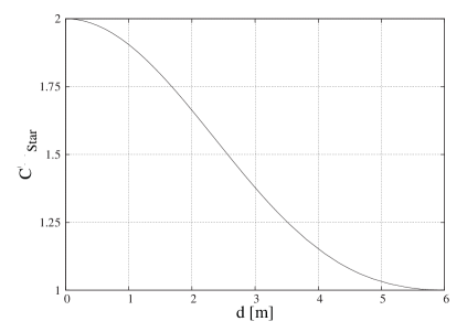
Figure 3: The normalized correlation function $C_{\rm Star}$ as given by Eq. (17) for the following parameter (Sirius): stellar radius $R=1.2\times 10^{9}\,{\rm m}$, distance between star and detectors $L=8.6\,{\rm lightyear}=8.136\times 10^{16}\,{\rm m}$, and wave-vector $k=2.15\times 10^{7}\,{\rm m}^{-1}$. By comparing with (18) we deduce an opening angle $\Theta=2\,R/L=2.9\times 10^{-8}\,{\rm rad}$.

2.1.2 Correlation function in the limit of heavy-ion collisions

In case of heavy-ion collisions (HIC) we have the following limits: $L\gg d_{AB}\gg r_{12}$, where $L$ is the distance between fireball and detectors, $r_{12}$ is the distance among two pointlike regions on the fireball’s surface and $d_{AB}$ is the distance between both detectors, see Fig.2. In these limits, the cosine-function in (LABEL:Introduction_26) can be considerably simplified and is given by

$$C_{\rm HIC}\left(\mbox{\boldmath$x$}_{1},\mbox{\boldmath$x$}_{2},\mbox{\boldmath$x$}_{A},\mbox{\boldmath$x$}_{B}\right) = 1+\cos\left(k\,\frac{\mbox{\boldmath$d$}_{AB}\cdot\mbox{\boldmath$r$}_{12}}{L}\right).$$ (19)

For comparison with the heavy-ion collision results we recall the practical relation $\mbox{\boldmath$q$}=\mbox{\boldmath$q$}_{AB}=k\,\mbox{\boldmath$d$}_{AB}/L$, because there the distance of the detectors, $d_{AB}$, is not measured directly. We recognize that the correlation function in the limits of heavy-ion collisions in (19) agrees with the correlation function in the limit for stars (14). Also in case of heavy-ion collisions one has to sum over all individual pointlike regions over the entire fireball created in the heavy-ion collision process. However, the description of HBT in heavy-ion collisions is more complicated than for stars, because the fireball expands rapidly in time and space, and therefore a simple two-dimensional integration procedure like in (16) is inapplicable, instead a four-dimensional description is necessary.

2.2 HBT effect in terms of quantum electrodynamics

The surprising discovery of quantum correlations of second-order in ordinary light by Hanbury Brown and Twiss came to pass when they applied photodetectors in the domain of the optical spectrum [1, 2]. The theoretical description of a localized absorption process of a photon by photodetectors (e.g. photodiodes, photomultipliers, CCD’s) implies the electromagnetic field to be considered as made of by photons instead of classical waves. One aspect thereof is the symmetrization of the photon wavefunction under coordinate-exchange of two indistinguishable photons, a term which, however, does not occur in classical electrodynamics. Accordingly, the use of a photon-counter implies that the electric radiation-field $\mbox{\boldmath$E$}\left(\mbox{\boldmath$r$},t\right)$ in (1) must have to be described as a second-quantized quantum-field, indicated by a hat: $\hat{\mbox{\boldmath$E$}}\left(\mbox{\boldmath$r$},t\right)$ [26, 27]:

$$\hat{\mbox{\boldmath$E$}}\left(\mbox{\boldmath$r$},t\right) = \hat{\mbox{\boldmath$E$}}^{\left(+\right)}\left(\mbox{\boldmath$r$},t\right)+\hat{\mbox{\boldmath$E$}}^{\left(-\right)}\left(\mbox{\boldmath$r$},t\right),$$ (20)

$$\hat{\mbox{\boldmath$E$}}^{\left(+\right)}\left(\mbox{\boldmath$r$},t\right) = +i\,\frac{{\rm e}^{+i\left(k\,r-\omega_{k}\,t\right)}}{k\,r}\sum\limits_{l=1}^{\infty}\sum\limits_{m=-l}^{l}\hat{a}_{lm}\;\mbox{\boldmath$g$}_{lm}\left(\theta,\phi\right),$$ (21)

$$\hat{\mbox{\boldmath$E$}}^{\left(-\right)}\left(\mbox{\boldmath$r$},t\right) = -i\,\frac{{\rm e}^{-i\left(k\,r-\omega_{k}\,t\right)}}{k\,r}\sum\limits_{l=1}^{\infty}\sum\limits_{m=-l}^{l}\hat{a}^{\dagger}_{lm}\;\mbox{\boldmath$g$}^{\ast}_{lm}\left(\theta,\phi\right).$$ (22)

By comparing the second-quantized electric field operator in (20) with the classical electric field in (1), one recognizes that there is formally a replacement of the classical amplitudes by operators : $\alpha_{lm}\rightarrow\hat{a}_{lm}$ and $\alpha^{\ast}_{lm}\rightarrow\hat{a}^{\dagger}_{lm}$, where $\hat{a}_{lm}^{\dagger}$ is the Hermitian adjoint of $\hat{a}_{lm}$. These photon-operators act in the Fock-space of photon states and obey commutator relations in angular-momentum space, given by [26, 27]:

$$\left[\hat{a}_{l_{1}m_{1}}\,,\,\hat{a}^{\dagger}_{l_{2}m_{2}}\right]_{-} = \omega_{k}\,\delta_{l_{1}l_{2}}\,\delta_{m_{1}m_{2}}\,,\quad\left[\hat{a}_{l_{1}m_{1}}\,,\,\hat{a}_{l_{2}m_{2}}\right]_{-}=0\,,\quad\left[\hat{a}^{\dagger}_{l_{1}m_{1}}\,,\,\hat{a}^{\dagger}_{l_{2}m_{2}}\right]_{-}=0\,.$$ (23)

The operator $\hat{a}^{\dagger}_{l_{1}m_{1}}$ creates one photon with angular-momentum $l_{1}m_{1}$, while the operator $\hat{a}_{l_{1}m_{1}}$ annihilates one photon with angular-momentum $l_{1}m_{1}$. In particular, the vacuum state is defined by $\hat{a}_{l_{1}m_{1}}|{\rm vac}\rangle=0$, and $|l_{1}m_{1}\rangle=\hat{a}_{l_{1}m_{1}}^{\dagger}|{\rm vac}\rangle$ represents a one-photon state, while $\displaystyle|l_{1}m_{1}\;l_{2}m_{2}\rangle=\frac{1}{\sqrt{2}}\,\hat{a}_{l_{1}m_{1}}^{\dagger}\hat{a}_{l_{2}m_{2}}^{\dagger}|{\rm vac}\rangle$ represents a two-photon state in the angular-momentum space. Accordingly, the positive-energy part (21) annihilates one photon localized at $r,\theta,\phi,t$ in coordinate-space, while the negative-energy part (22) creates one photon localized at $r,\theta,\phi,t$ in coordinate-space.

Like in the classical case, we assume the detectors are sensitive only to those photons which are polarized in an arbitrary but fixed unit-direction $e$, and consider the vector-component of the electric field-operator in this direction: $\hat{\cal E}\left(\mbox{\boldmath$r$},t\right)=\mbox{\boldmath$e$}\cdot\hat{\mbox{\boldmath$E$}}\left(\mbox{\boldmath$r$},t\right)$ [16]. One individual mode of the electric field-operator is then given by

$$\hat{\cal E}\left(\mbox{\boldmath$r$},t\right) = \hat{\cal E}^{\left(+\right)}\left(\mbox{\boldmath$r$},t\right)+\hat{\cal E}^{\left(-\right)}\left(\mbox{\boldmath$r$},t\right)\,,$$ (24)

$$\hat{\cal E}^{\left(+\right)}\left(\mbox{\boldmath$r$},t\right) = +i\,\frac{{\rm e}^{+i\left(k\,r-\omega_{k}\,t\right)}}{k\,r}\hat{a}_{lm}\;{\it g}_{\,lm}\left(\theta,\phi\right),$$ (25)

$$\hat{\cal E}^{\left(-\right)}\left(\mbox{\boldmath$r$},t\right) = -i\,\frac{{\rm e}^{-i\left(k\,r-\omega_{k}\,t\right)}}{k\,r}\hat{a}^{\dagger}_{lm}\;{\it g}^{\ast}_{\,lm}\left(\theta,\phi\right).$$ (26)

The field-operator in Eq. (24) is the quantum-field analogon of the classical electric field in Eq. (2).

The theory of HBT effect in terms of quantum electrodynamics has been worked out by Glauber in a series of articles [16, 17, 18]. We shall recall some parts of this theory which are relevant for our investigation.

The initial state before a one-photon detection at time $t$ is denoted by $|i\rangle$, and the final state after detection is denoted by $|f\rangle$ which contains one photon less because it has been absorbed by the detector located at $\mbox{\boldmath$x$}_{A}$. The final states form a complete set of states, $\sum_{f}|f\rangle\,\langle f|={\bf 1}1$. The corresponding amplitude for a one-photon absorption is given by the following matrix element: $\langle f|\hat{\cal E}^{\left(+\right)}\left(\mbox{\boldmath$x$}_{A},t\right)|i\rangle$. The probability of this process is given by the square of the absolute value of this amplitude (Fermi’s golden rule), $W^{\left(1\right)}_{if}=\left|\langle f|\hat{\cal E}^{\left(+\right)}\left(\mbox{\boldmath$x$}_{A},t\right)|i\rangle\right|^{2}$. If one wants to determine the total probability that one photon is absorbed at time $t$ by an ideal photon detector located at $\mbox{\boldmath$x$}_{A}$ and irrespective of the final state, then one has to sum over all final states and obtains, cf. Eq. (2.15) in [16]:

$$W^{\left(1\right)}_{i}\left(\mbox{\boldmath$x$}_{A},t\right) = \sum\limits_{f}\left|\langle f|\hat{\cal E}^{\left(+\right)}\left(\mbox{\boldmath$x$}_{A},t\right)|i\rangle\right|^{2}=\langle i|\hat{\cal E}^{\left(-\right)}\left(\mbox{\boldmath$x$}_{A},t\right)\hat{\cal E}^{\left(+\right)}\left(\mbox{\boldmath$x$}_{A},t\right)|i\rangle\,,$$ (27)

where in the last term a summation over the complete set of final states has been performed. If the initial state $|i\rangle$ is not a pure state but a statistical mixture of states (thermal bath of photons), then the initial state is described by a statistical operator $\hat{\rho}$ and the average in (27) has to be determined by the trace over the density operator: $\langle i|\hat{\cal O}|i\rangle\rightarrow{\rm Tr}\left(\hat{\rho}\,\hat{\cal O}\right)$. Similarly, in case of two-photon detection at time $t$ by two detectors located at $\mbox{\boldmath$x$}_{A}$ and $\mbox{\boldmath$x$}_{B}$, the amplitude of this process reads $\langle f|\hat{\cal E}^{\left(+\right)}\left(\mbox{\boldmath$x$}_{B},t\right)\,\hat{\cal E}^{\left(+\right)}\left(\mbox{\boldmath$x$}_{A},t\right)|i\rangle,$ and the probability of this process is (Fermi’s golden rule) $W^{\left(2\right)}_{if}=\left|\langle f|\hat{\cal E}^{\left(+\right)}\left(\mbox{\boldmath$x$}_{A},t\right)\hat{\cal E}^{\left(+\right)}\left(\mbox{\boldmath$x$}_{B},t\right)|i\rangle\right|^{2}$. The total probability, that two photons are absorbed at time $t$ by two ideal photon detectors located at $\mbox{\boldmath$x$}_{A}$ and $\mbox{\boldmath$x$}_{B}$, and irrespective of the final state is given by, cf. Eq. (2.17) in [16]:

$$W^{\left(2\right)}_{i}\left(\mbox{\boldmath$x$}_{A},\mbox{\boldmath$x$}_{B}\right) = \sum\limits_{f}\left|\langle f|\hat{\cal E}^{\left(+\right)}\left(\mbox{\boldmath$x$}_{B},t\right)\,\hat{\cal E}^{\left(+\right)}\left(\mbox{\boldmath$x$}_{A},t\right)|i\rangle\right|^{2}$$ (28)

$$= \langle i|\hat{\cal E}^{\left(-\right)}\left(\mbox{\boldmath$x$}_{A},t\right)\,\hat{\cal E}^{\left(-\right)}\left(\mbox{\boldmath$x$}_{B},t\right)\,\hat{\cal E}^{\left(+\right)}\left(\mbox{\boldmath$x$}_{B},t\right)\,\hat{\cal E}^{\left(+\right)}\left(\mbox{\boldmath$x$}_{A},t\right)|i\rangle\,,$$

where in the last line a summation over the complete set of final states has been performed. The expression in (28) describes basically the correlation of a two-photon absorption process, namely one photon is absorbed at detector position $\mbox{\boldmath$x$}_{A}$ and at the same instant of time another photon is absorbed at detector position $\mbox{\boldmath$x$}_{B}$. In this sense one can call this expression correlation function. For a theoretical description of real correlation experiments it is convenient to consider, first of all, two pintlike regions located at $\mbox{\boldmath$x$}_{1}$ and $\mbox{\boldmath$x$}_{2}$ on the star’s surface, each of which emits one spherical photon-mode. Then, we arrive at the following correlation function,

$$C\left(\mbox{\boldmath$x$}_{1},\mbox{\boldmath$x$}_{2},\mbox{\boldmath$x$}_{A},\mbox{\boldmath$x$}_{B}\right) \!\!=\!\! \frac{\sum\limits_{f}\left|\langle f|\hat{\cal E}^{\left(+\right)}\left(\mbox{\boldmath$x$}_{1},\mbox{\boldmath$x$}_{2},\mbox{\boldmath$x$}_{B}\right)\,\hat{\cal E}^{\left(+\right)}\left(\mbox{\boldmath$x$}_{1},\mbox{\boldmath$x$}_{2},\mbox{\boldmath$x$}_{A}\right)|i\rangle\right|^{2}}{\sum\limits_{f}\left|\langle f|\hat{\cal E}^{\left(+\right)}\left(\mbox{\boldmath$x$}_{1},\mbox{\boldmath$x$}_{2},\mbox{\boldmath$x$}_{B}\right)|i\rangle\right|^{2}\sum\limits_{f}\left|\langle f|\hat{\cal E}^{\left(+\right)}\left(\mbox{\boldmath$x$}_{1},\mbox{\boldmath$x$}_{2},\mbox{\boldmath$x$}_{A}\right)|i\rangle\right|^{2}}\,,$$ (29)

where we also have introduced a normalized form of (28), cf. Eq. (4.3) in [16]. The correlation function (29) determines the rate of coincidences in the photon count rate of two detectors at $\mbox{\boldmath$x$}_{A}$ and $\mbox{\boldmath$x$}_{B}$, and is the quantum-field theoretical analog of the classical correlator (8) for two pointlike regions of thermal radiation. In order to determine the correlation function in (29), the electric field-operators in (29) can been obtained by a second-quantization procedure of the classical expressions in (3) - (7) with the aid of formal replacements of the classical amplitudes by operators $\alpha_{lm}\rightarrow\hat{a}_{lm}$ and $\alpha^{\ast}_{lm}\rightarrow\hat{a}^{\dagger}_{lm}$,

$$\hat{\cal E}^{\left(+\right)}\left(\mbox{\boldmath$x$}_{1},\mbox{\boldmath$x$}_{2},\mbox{\boldmath$x$}_{A},t\right) = \hat{\cal E}^{\left(+\right)}\left(\mbox{\boldmath$x$}_{1},\mbox{\boldmath$x$}_{A},t\right)+\hat{\cal E}^{\left(+\right)}\left(\mbox{\boldmath$x$}_{2},\mbox{\boldmath$x$}_{A},t\right),$$ (30)

where these two positive-energy field-operators

$$\hat{\cal E}^{\left(+\right)}\left(\mbox{\boldmath$x$}_{1},\mbox{\boldmath$x$}_{A},t\right) = +i\,\hat{a}_{l_{1}m_{1}}\,{\it g}_{\,l_{1}m_{1}}\,\frac{{\rm exp}\left[+i\left(k_{1}\,\left|\mbox{\boldmath$x$}_{A}-\mbox{\boldmath$x$}_{1}\right|-\omega_{k_{1}}\,t\right)\right]}{k_{1}\;\left|\mbox{\boldmath$x$}_{A}-\mbox{\boldmath$x$}_{1}\right|}\,,$$ (31)

$$\hat{\cal E}^{\left(+\right)}\left(\mbox{\boldmath$x$}_{2},\mbox{\boldmath$x$}_{A},t\right) = +i\,\hat{a}_{l_{2}m_{2}}\,{\it g}_{\,l_{2}m_{2}}\,\frac{{\rm exp}\left[+i\left(k_{2}\,\left|\mbox{\boldmath$x$}_{A}-\mbox{\boldmath$x$}_{2}\right|-\omega_{k_{2}}\,t\right)\right]}{k_{2}\;\left|\mbox{\boldmath$x$}_{A}-\mbox{\boldmath$x$}_{2}\right|}\,.$$ (32)

The field-operator at detector positon $\mbox{\boldmath$x$}_{B}$ can be obtained by a replacement of $\mbox{\boldmath$x$}_{A}$ by $\mbox{\boldmath$x$}_{B}$ in Eqs. (30) - (32). In the initial state in the nominator and denominator in (29) there are two photons: $\displaystyle|i\rangle=\frac{1}{\sqrt{2}}|l_{1}m_{1}\;l_{2}m_{2}\rangle$. In the nominator in (29) the final state is the vacuum state $\langle f|=\langle{\rm vac}|$, while in the denominator in (29) the final state is a one-photon state, either $\langle f|=\langle l_{1}m_{1}|$ or $\langle f|=\langle l_{2}m_{2}|$, depending on which photon has not been detected. We assume that both emitted photons have the same energy $k_{1}=k_{2}$ but, for simplicity, here we take either $l_{1}\neq l_{2}$ or $m_{1}\neq m_{2}$. Then, by inserting the field-operators (30) into (29) we obtain the following expression for the correlation function:

$$C\left(\mbox{\boldmath$x$}_{1},\mbox{\boldmath$x$}_{2},\mbox{\boldmath$x$}_{A},\mbox{\boldmath$x$}_{B}\right) = \left|\Psi_{12}\right|^{2}\,,$$ (33)

where the photon wavefunction is given by

$$\Psi_{12}\left(\mbox{\boldmath$x$}_{1},\mbox{\boldmath$x$}_{2},\mbox{\boldmath$x$}_{A},\mbox{\boldmath$x$}_{B}\right) = \frac{1}{\sqrt{2}}\left[{\rm e}^{i\,k\,\left|\mbox{\scriptsize\boldmath$x_{1}$}-\mbox{\scriptsize\boldmath$x_{A}$}\right|}\;{\rm e}^{i\,k\,\left|\mbox{\scriptsize\boldmath$x_{2}$}-\mbox{\scriptsize\boldmath$x_{B}$}\right|}+{\rm e}^{i\,k\,\left|\mbox{\scriptsize\boldmath$x_{2}$}-\mbox{\scriptsize\boldmath$x_{A}$}\right|}\;{\rm e}^{i\,k\,\left|\mbox{\scriptsize\boldmath$x_{1}$}-\mbox{\scriptsize\boldmath$x_{B}$}\right|}\right]\,.$$ (34)

This wavefunction is valid both for heavy-ion collisions and stars, and symmetric under exchange of source-coordinates $\mbox{\boldmath$x$}_{1}\leftrightarrow\mbox{\boldmath$x$}_{2}$ and detector-coordinates $\mbox{\boldmath$x$}_{A}\leftrightarrow\mbox{\boldmath$x$}_{B}$. After an experimental measurement the wavefunction collapses and disappears completely. Let us also recall, that $\Psi_{12}$ is not an observable, while $\left|\Psi_{12}\right|^{2}$ can be determined by experiments. For the absolute square of photon wavefunction (34) we obtain

$$\left|\Psi_{12}\right|^{2} = 1+\cos\bigg{[}k\Big{(}\left|\mbox{\boldmath$x$}_{1}-\mbox{\boldmath$x$}_{A}\right|+\left|\mbox{\boldmath$x$}_{2}-\mbox{\boldmath$x$}_{B}\right|-\left|\mbox{\boldmath$x$}_{2}-\mbox{\boldmath$x$}_{A}\right|-\left|\mbox{\boldmath$x$}_{1}-\mbox{\boldmath$x$}_{B}\right|\Big{)}\bigg{]}\,.$$ (35)

We recognize, that the absolute square of wavefunction in (35) equals the classical correlation function given by (LABEL:Introduction_26).

The symmetrization of wavefunction in (34) is a fundamental law of quantum mechanics and is independent of any specific performance of an experiment. In other words, the photons, during their propagation from the star (or fireball of a heavy-ion collision process) to the detectors, do not take care about the existence of some detectors anywhere in the universe. For instance, in real HBT experiments in heavy-ion collisions one might want to install about $3000$ detectors around the fireball in order to minimize the loss of photons which have been emitted by the fireball and to improve the statistics and accuracy. Finally, one is searching in the experimental data for all two-photon correlations (HBT effect) measured by any two detectors among these $3000$ detectors. But the photon (or pion) wavefunction is symmetric in the coordinates of the fireball as well as in the coordinates of the final two detectors. The same symmetry exists in case of HBT measurements for stars. However, different experiments have different geometrical configurations. Depending on these specific experimental configurations, see Fig. 4, some parts of the wavefunction in (34) become important, while other parts in the wavefunction become negligible. For instance, in case of stars the wave-function is given by Eq. (1) in [22], while in case of heavy-ion collisions the wave-function is given by Eq. (8) in [22].

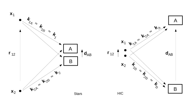
Figure 4: The extreme limits for the momenta. Left pannel: photon-momenta in case of stars $r_{12}\gg d_{AB}$. In this limit the wavefunction $\Psi_{12}$ in (34) simplifies to $\Psi_{12}^{\rm Star}$ in (36). Right pannel: photon-momenta in case of heavy-ion collisions $r_{12}\ll d_{AB}$. In this limit the wavefunction $\Psi_{12}$ in (34) simplifies to $\Psi_{12}^{\rm HIC}$ in (39).

Actually, more important is the absolute square of the wave-function. Especially, like in the classical theory, there are two relevant limits for the absolute value in Eq. (35), stars and heavy-ion collisions, which will be considered in the following.

2.2.1 Wavefunction for stars

In case of a star we have the following limits; see left pannel of Fig. 4: $L\gg r_{12}\gg d_{AB}$, where $L$ is the distance between star and detectors, $r_{12}$ is the distance among two pointlike regions on the star’s surface, and $d_{AB}$ is the distance between both detectors, see Fig.2. In these limits, photon wavefunction in (34) can considerably be simplified and is given by; cf. [22]:

$$\Psi_{12}^{\rm Star} = \frac{1}{\sqrt{2}}\bigg{[}{\rm e}^{i\left[\mbox{\scriptsize\boldmath$k_{1}$}\cdot\left(\mbox{\scriptsize\boldmath$x_{A}$}-\mbox{\scriptsize\boldmath$x_{1}$}\right)+\mbox{\scriptsize\boldmath$k_{2}$}\cdot\left(\mbox{\scriptsize\boldmath$x_{B}$}-\mbox{\scriptsize\boldmath$x_{2}$}\right)\right]}+{\rm e}^{i\left[\mbox{\scriptsize\boldmath$k_{1}$}\cdot\left(\mbox{\scriptsize\boldmath$x_{B}$}-\mbox{\scriptsize\boldmath$x_{1}$}\right)+\mbox{\scriptsize\boldmath$k_{2}$}\cdot\left(\mbox{\scriptsize\boldmath$x_{A}$}-\mbox{\scriptsize\boldmath$x_{2}$}\right)\right]}\bigg{]}\,,$$ (36)

where the wave-vector $\mbox{\boldmath$k$}_{1}$ is directed from spatial coordinate $\mbox{\boldmath$x$}_{1}$ of the star’s surface to detector A or B, and wave-vector $\mbox{\boldmath$k$}_{2}$ is directed from spatial coordinate $\mbox{\boldmath$x$}_{2}$ of the star’s surface to detector A or B. The derivation of Eq. (36) from Eq. (34) can be performed like in Section 5. The square of absolute value of this wavefunction is given by

$$\left|\Psi_{12}^{\rm Star}\right|^{2} = 1+\cos\left(k\,\frac{\mbox{\boldmath$d$}_{AB}\cdot\mbox{\boldmath$r$}_{12}}{L}\right),$$ (37)

where $\mbox{\boldmath$d$}_{AB}=\mbox{\boldmath$x$}_{B}-\mbox{\boldmath$x$}_{A}$ is the vector from detector A towards detector B, and $\mbox{\boldmath$r$}_{12}=\mbox{\boldmath$x$}_{2}-\mbox{\boldmath$x$}_{1}$ is the vector from surface-point $\mbox{\boldmath$x$}_{1}$ towards the surface-point $\mbox{\boldmath$x$}_{2}$ of the star, $k=\left|\mbox{\boldmath$k$}_{1}\right|=\left|\mbox{\boldmath$k$}_{2}\right|$, and we have used the relation $\displaystyle\mbox{\boldmath$k$}_{2}-\mbox{\boldmath$k$}_{1}=k\,\frac{\mbox{\boldmath$r$}_{12}}{L}$ which is valid for the geometry of stars; see left pannel in Fig. 4. Obviously, (37) equals the classical expression obtained in (14).

Like in the classical case, see Eq. (16), in order to obtain the correlation function for the whole radiation field of a star, one has to sum over all individual pointlike regions over the entire surface of the star facing the observer:

$$C_{\rm Star}\left(\mbox{\boldmath$x$}_{A},\mbox{\boldmath$x$}_{B}\right) = \frac{1}{A_{\rm star}^{2}}\int_{A_{\rm star}}d^{2}x_{1}\;\int_{A_{\rm star}}d^{2}x_{2}\;\left|\Psi^{\rm Star}_{12}\right|^{2}$$ (38)

$$= 1+\frac{4\,L^{2}}{k^{2}\,d_{AB}^{2}\,R^{2}}\,J_{1}^{2}\left(\frac{k\,R\,d_{AB}}{L}\right),$$

which is obviously the same expression for the correlation function for stars in Eq. (17), previously obtained in the treatment in terms of classical electrodynamics. As specific example, Eq. (38) reflects the analogon of Siegert relation in quantum electrodynamics, first obtained by Glauber, cf. Eq. (10.26) in [18], and in general valid for incoherent light.

2.2.2 Wavefunction for heavy-ion collisions

In case of heavy-ion collisions we have the following limits; see right pannel of Fig. 4: $L\gg d_{AB}\gg r_{12}$, where $L$ is the distance between fireball and detectors, $r_{12}$ is the distance among two pointlike regions on the fireball’s surface and $d_{AB}$ is the distance between both detectors, see Fig.2. In these limits, the photon wavefunction in (34) can considerably be simplified and is given by; cf. [22]:

$$\Psi_{12}^{\rm HIC} = \frac{1}{\sqrt{2}}\bigg{[}{\rm e}^{i\left[\mbox{\scriptsize\boldmath$k_{A}$}\cdot\left(\mbox{\scriptsize\boldmath$x_{A}$}-\mbox{\scriptsize\boldmath$x_{1}$}\right)+\mbox{\scriptsize\boldmath$k_{B}$}\cdot\left(\mbox{\scriptsize\boldmath$x_{B}$}-\mbox{\scriptsize\boldmath$x_{2}$}\right)\right]}+{\rm e}^{i\left[\mbox{\scriptsize\boldmath$k_{A}$}\cdot\left(\mbox{\scriptsize\boldmath$x_{A}$}-\mbox{\scriptsize\boldmath$x_{2}$}\right)+\mbox{\scriptsize\boldmath$k_{B}$}\cdot\left(\mbox{\scriptsize\boldmath$x_{B}$}-\mbox{\scriptsize\boldmath$x_{1}$}\right)\right]}\bigg{]}\,,$$ (39)

where the wave-vector $\mbox{\boldmath$k$}_{A}$ is directed from the fireball’s surface towards detector A, the wave-vector $\mbox{\boldmath$k$}_{B}$ is directed from the fireball’s surface towards detector B. The square of absolute value of this wavefunction is given by

$$\left|\Psi_{12}^{\rm HIC}\right|^{2} = 1+\cos\left(k\,\frac{\mbox{\boldmath$d$}_{AB}\cdot\mbox{\boldmath$r$}_{12}}{L}\right),$$ (40)

where $\mbox{\boldmath$r$}_{12}=\mbox{\boldmath$x$}_{2}-\mbox{\boldmath$x$}_{1}$ is the vector from one surface-point $\mbox{\boldmath$x$}_{1}$ of the fireball of HIC to another surface-point $\mbox{\boldmath$x$}_{2}$ of the fireball, $k=\left|\mbox{\boldmath$k$}_{A}\right|=\left|\mbox{\boldmath$k$}_{A}\right|$ is the absolute value of wave-vector of the photons, and we have used $\displaystyle\mbox{\boldmath$k$}_{B}-\mbox{\boldmath$k$}_{A}=k\,\frac{\mbox{\boldmath$d$}_{AB}}{L}$ which is valid for the geometry of heavy-ion collisions; see right pannel in Fig. 4.

We note that (40) equals the corresponding classical expression obtained in (19). Like in the classical case, the absolute square of wavefunction in the limits of heavy-ion collisions in (40) agrees with the the absolute square of wavefunction in the limit for stars (37). Let us recall here that the fireball created by a heavy-ion collision expands rapidly in time and space, hence the two-dimensional integration procedure in (38) has to be replaced by an invariant four-dimensional approach, which will briefly be discussed in the next Section.

2.3 HBT effect for binary stars

In the previous sections it has been shown that classical electrodynamics and quantum-electrodynamical treatment leads to the same expressions for the correlation function of two pointlike sources, see Eq. (14). Therefore, we can just apply any of these expressions in order to derive the correlation function for binary stars, given by

$$C_{\rm Binary}\left(\mbox{\boldmath$x$}_{A},\mbox{\boldmath$x$}_{B}\right) = \frac{1}{2\,A_{\rm star}^{2}}\;\int d^{2}x_{1}\;\int d^{2}x_{2}\;\left[1+\cos\left(k\,\frac{\mbox{\boldmath$r$}_{12}\cdot\mbox{\boldmath$d$}_{AB}}{L}\right)\right]\,,$$ (41)

where the regions of integrations are elucidated in Fig. 5.

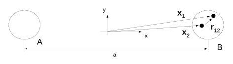
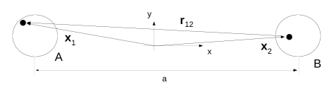
Figure 5: The both components of the binary system are denoted by $A$ and $B$. These figures elucidate the region of integration in Eq. (41).

The integration in (41) yields for the correlation function for binary stars the following expression:

$$C_{\rm Binary}\left(\mbox{\boldmath$x$}_{A},\mbox{\boldmath$x$}_{B}\right) = 1+\frac{4\,L^{2}}{k^{2}\,d_{AB}^{2}\,R^{2}}\,J_{1}^{2}\left(\frac{k\,R\,d_{AB}}{L}\right)\left(1+\cos\frac{k\,a\left(t\right)\,d_{AB}}{L}\right),$$ (42)

which is valid for $a\left(t\right)\geq 2\,R$; the extreme case $a\left(t\right)<2\,R$ is not relevant for our investigation. The term in (42) which is not proportional to the cosine-function agrees with (38), and describes the standard HBT effect for stars, that means photons from star A are correlated with each other and photons from star B are correlated with each other. The term in (42) which is proportional to the cosine-function describes the HBT effect due to the binary system, that means photons from star A and photons from star B are correlated with each other.

Two configurations are on the scope of our investigation. First, the case of inclination $i=0$, where for circular orbits (eccentricity $e=0$) the apparent distance between both stars as seen from the observer is simply given by

$$a\left(t\right)=A={\rm const}\,.$$ (43)

Second, the case of edge-on binaries (inclination $\displaystyle i=\pi/4$), where for circular orbits the time-dependent distance $a\left(t\right)$ between both stars as seen from an observer takes the form

$$a\left(t\right) = A\,\cos\left(\frac{2\,\pi}{\mathcal{T}}\,\,t\right)\quad{\rm for}\quad a\left(t\right)\geq 2\,R.$$ (44)

Here, $t$ is the time, while $\mathcal{T}$ is the orbital period, given by

$$\mathcal{T} = 2\,\pi\,\sqrt{\frac{A^{3}}{G\,\left(M_{A}+M_{B}\right)}}\,,$$ (45)

where $A$ is the semi-major axis, and $\displaystyle G=6.67\times 10^{-11}\,\frac{{\rm m}^{3}}{{\rm kg}\,{\rm s}^{2}}$ is the gravitational constant.

We will show that these results for the correlation function for stars (38) and for binary stars (42) can be reproduced by means of the more sophisticated approach of differential HBT-method, which has originally been introduced for analyzing the HBT effect in the fireball of heavy-ion collisions [11, 12, 13].

3 HBT in heavy-ion-physics and astrophysics

By means of the HBT effect in astrophysics one may determine the spatial size of a star or the distance between the components of a binary system, while the HBT analysis in heavy-ion physics allows to get information about the space-time structure and evolution of the fireball created in heavy-ion collisions. But both approaches differ significantly. The HBT approach used in heavy-ion physics is more involved and more general than in case of astrophysics, simply because the hot and dense hadronic fireball expands rapidly in time and space on a timescale of about $10^{-22}\,...\,10^{-21}\,{\rm seconds}$, while a star emits continuously thermal radiation and the star’s surface does not alter significantly over a very long period of time of about $10^{16}\,{\rm seconds}$. Therefore, a simple two-dimensional integration procedure like in (16) is inapplicable in heavy-ion physics, instead a four-dimensional description is necessary. Both appraches are compared and the conditions are elucidated about how to modify the HBT analysis used in HIC for the case of astrophysics.

HBT analysis in heavy-ion physics:

Since the fireball expands rapidly, in heavy-ion physics the second-order correlation function in (16) is generalized into a four-dimensional description in momentum-space, see e.g. [32], where it reads:

$$C\left(k_{A},k_{A}\right) = \frac{P_{2}\left(k_{A},k_{B}\right)}{P_{1}\left(k_{A}\right)P_{1}\left(k_{B}\right)}\;,$$ (46)

where $k_{A}=\left(\omega_{k_{A}},\mbox{\boldmath$k$}_{A}\right)$ and $k_{B}=\left(\omega_{k_{B}},\mbox{\boldmath$k$}_{B}\right)$ are the four-momenta of the two photons and $P_{1}$ and $P_{2}$ are the inclusive one-photon and two-photon distribution function, respectively. That means, $P_{1}\left(k_{A}\right)$ is the probability of detecting one photon of momentum $k_{A}$ in detector A or B, $P_{1}\left(k_{B}\right)$ is the probability of detecting one photon of momentum $k_{B}$ in detector A or B, and $P_{2}\left(k_{A},k_{B}\right)$ is the probability of detecting two coincident photons of wavenumbers $k_{A}$ and $k_{B}$ in detectors A and B. Let’s assume the photons are emitted at two points on the fireball’s surface, $x_{1}=\left(t_{1},\mbox{\boldmath$x$}_{1}\right)$ and $x_{2}=\left(t_{2},\mbox{\boldmath$x$}_{2}\right)$. Then, the one-photon and two-photon distribution function is then given by

$$P_{1}\left(k_{A}\right) = \int d^{4}x_{1}\;S\left(x_{1},k_{A}\right),\quad P_{1}\left(k_{B}\right)=\int d^{4}x_{1}\;S\left(x_{1},k_{B}\right),$$ (47)

$$P_{2}\left(k_{A},k_{B}\right) = \int d^{4}x_{1}\,d^{4}x_{2}\;S\left(x_{1},k_{A}\right)S\left(x_{2},k_{B}\right)\left|\Psi_{12}\right|^{2}\,,$$ (48)

where $\Psi_{12}$ is the two-photon wavefunction in (34) and its absolute square in (35), and the functions $S\left(x_{1},k_{A}\right)$ and $S\left(x_{2},k_{B}\right)$ are the socalled photon emission functions, a term originally introduced in heavy-ion physics and which will be considered in the next Section.

In heavy-ion collisions the HBT effect was originally been used for the same purpose as in astrophysics, namely the determination of the system size by measuring the correlations of bosons (pion pair correlations and later photon pair correlations) which are emitted from the expanding fireball created by the heavy-ion collision [3]. Up to now, the HBT analysis remains the only experimental and model-independent approach to determine the size af the expanding fireball. Ever since, the effect of photon (or pion correlations) has become a fundamental aspect not only in field of quantum optics, but also in the theory and experiment of heavy-ion (or nucleon-nucleon) collisions. That means, similar second-order correlation functions (46) have also been measured in heavy-ion collisions for pion-correlations [4, 5] (where $\Psi_{12}$ would then be the two-pion wavefunction and the four-dimensional integrations would run over the fireball).

Todays highly sophisticated high energy heavy-ion experiments can even detect the ellipsoidal shape of the fireball and also its tilt by means of the HBT effect [6, 33]. At present collision energies the angular momentum and rotation of the hot and dense fireball is becoming a dominant feature of heavy-ion collisional processes, and the possibility to analyze such effects by the so-called differential HBT method was subject of the investigations in [11, 12, 13].

In heavy-ion reactions numerous particles are registered, of the order of thousand, in every single collision event. The timespan of the reaction is of the order of $10\,{\rm fm}/c$ just as the size of the system. So, the particles emitted and observed in one collision event are considered as contemporary, and interacting with each other. Consequently an event by event measurement registers an M-particle correlation (where M is the bserved multiplicity of the event). For the second-order correlation function every pair is selected from the M particles and this provides the probability distribution $P_{2}\left(k_{A},k_{B}\right)$ which allows to determine the second-order correlation function in (46).

HIB analysis in astrophysics:

In order to exploit the advanced machinery of HBT analysis developed in heavy-ion physics, in our subsequent investigation we will start to consider the correlator in (46) instead (16). The results of such an approach will finally yield similar expressions for the correlator as given by Eq. (38) for stars and by Eq. (42) for binaries. In doing so, several aspects have carefully to be accounted for.

First, as mentioned above, in case of stars and binary stars we face a continuous emission of thermal radiation in time. We have to assume that the luminosity from the stars is big enough, so that in a correlation time period we have sufficient amount of photons emitted in the direction of the observer so that the observable multiplicity, $M\gg 4$. According to the investigations in [34] we can savely assume that this requirement is obeyed for many stars located in the neighborhood of the Solar system; e.g. from Sirius $10^{6}{\rm photons}/{\rm cm}^{2}\,{\rm sec}$ arrive the Earth’s surface. Then, the subsequent analysis can be repeated in every such time interval, similarly to subsequent collision events in heavy-ion reactions. However, in case of faint and optically not resolvable binaries, the luminosity might not be too large, so it is also important that the detection efficiency should be as high as possible. In this respect we mention that most modern optical technologies allow to generate CCD detectors with a plane of about $1\,{\rm square-meter}$, as used for instance in the ESA astrometry mission Gaia [35].

Second, we have to account for the fact, that the opacity of a star is so extremely high that the visible photons do not originate from inner regions of the star but from the thin photosphere of the star, that is to say from the two-dimensional surface. Accordingly, the HBT approach used in heavy-ion physics has to be modified for the case of astrophysics, by simplifying the four-dimensional integrals in (47) - (48) by integrals which run over the two-dimensional hyper-surface of stars.

Third, the wavefunction in (34) is valid both for the geometry of HIC (i.e. $d_{AB}\gg R$ and $R\ll L$) and for the geometry of astrophysics (i.e. $d_{AB}\ll R$ and $R\ll L$), and will be simplified and designed for the specific case of stars, cf. considerations in Section 2. These issues will be the subject of Section 4 and Section 5.

4 The Emission Function

Let us consider the photon emission function $S\left(x,k\right)$ which is a fundamental ingredient in the correlation functions in (46) via Eqs. (47) - (48). The photon emission function, frequently called sourcefunction, is the probability distribution of emitting a photon from the source point $x^{\mu}=\left(ct,\mbox{\boldmath$x$}\right)$ with four-momenta $k^{\mu}=\left(k^{0},\mbox{\boldmath$k$}\right)$, that means the number of photons, $\Delta N$, emitted in the phase-space element $\Delta^{3}x\,\Delta^{3}k$ per unit time $\Delta t$. A Lorentz invariant scalar can be obtained by multiplying the photon-energy $k^{0}=\omega_{k}$ of the emitted photons:

$$S\left(x,k\right) = k^{0}\frac{\Delta N}{\Delta t\,\Delta^{3}x\,\Delta^{3}k}\,.$$ (49)

Accordingly, the total number of photons is given by the summation over the entire space-time and momentum-space:

$$N = \int d^{4}x\int\frac{d^{3}k}{k^{0}}S\left(x,k\right).$$ (50)

For the calculation of the photon emission function in (49) one needs the photon four-current, defined by [36]:

$$N^{\mu}(x) = \int k^{\mu}\frac{d^{3}k}{k^{0}}f(x,k)\,,$$ (51)

where $f(x,k)$ is the invariant scalar phase-space density distribution (black body distribution) of the emitted photons,

$$f\left(x,k\right) = \frac{g_{\gamma}}{\left(2\pi\right)^{3}}\frac{1}{\exp\left(k^{\mu}\,u_{\mu}/T\right)-1}\,,$$ (52)

where the degeneracy-factor $g_{\gamma}=2$ accounts for the two polarizations of the photons. This single particle distribution depends on the local four-velocity $u^{\mu}(x)$ of the light-source. In order to obtain the total number of photons crossing a space-time hyper-surface $\Sigma$, we have to integrate over all momenta and over the entire surface:

$$N = \int_{\Sigma}\left[\int\frac{d^{3}k}{k^{0}}\,k^{\mu}\,f\left(x,k\right)\right]d\Sigma_{\mu}\,,$$ (53)

where $d\Sigma_{\mu}$ is an infinitesimal three-dimensional surface-element. By not performing the momentum integral in (53) we recover the invariant triple differential cross section by the Cooper-Frye formula [37]:

$$E\frac{dN}{d^{3}k} = \int_{\Sigma}f\left(x,k\right)\ k^{\mu}d\Sigma_{\mu}\,,$$ (54)

with $E=k^{0}$. On account of Eqs. (50) and (53), we get an integral relation between photon sourcefunction $S\left(x,k\right)$ and photon density distribution $f\left(x,k\right)$ as follows:

$$\int d^{4}x\,S\left(x,k\right) = \int_{\Sigma}\,f\left(x,k\right)\,k^{\mu}\,d\Sigma_{\mu}\,.$$ (55)

In the r.h.s. of Eqs. (53) - (55) it is assumed that the emission takes place through a three-dimensional hyper-surface $\Sigma$ with the normal vector $d\Sigma_{\mu}=d\Sigma_{\mu}(x)$. The hyper-surface is bordered by the outgoing light-cone, so all emitted particles should cross the hyper-surface. We are interested in the hypersurface $x^{0}={\rm const.}$. Then, for time-like surface we have $d\Sigma_{\mu}=dx\,dy\,dz\,\hat{\sigma}_{\mu}$, with $\hat{\sigma}_{\mu}$ being a dimensionless unit four-vector. We will assume the simplest case for the time-like normal $\hat{\sigma}_{\mu}=\left(1,0,0,0\right)$, but actually we do not need this requirement to determine correlation function since the invariant scalar $k^{\mu}\,\hat{\sigma}_{\mu}$ cancels in the normalized correlator. Then, according to relation (55) and in virtue of Eq. (52) the source-function can be parametrized as follows; cf. [11, 39]:

$$S\left(x,k\right) = \frac{2}{\left(2\pi\right)^{3}}\,\frac{\gamma_{s}}{\exp\left(k^{\mu}\,u_{\mu}\left(x\right)/T\left(x\right)\right)-1}\,H\left(t\right)\,G\left(x,y,z\right)\,k^{\mu}\,\hat{\sigma}_{\mu}(x)\,,$$ (56)

where $\gamma_{s}=\sqrt{1-v_{s}^{2}}$ is the Lorentz factor with $v_{s}=\left|\mbox{\boldmath$v$}_{s}\right|$ being the absolute value of spatial velocity of the source; let us recall that the chemical potential for photons is zero (i.e. fugacity factor equals $1$). The function $H\left(t\right)$ governs the time-dependence of photon emission, which in case of heavy-ion collisions is usually described by a delta-function (sudden freeze-out) or an exponentially decreasing Gauss-function (gradually freeze-out), e.g. [11], because the fireball emits photons during a small time-intervall around the freeze-out time $t_{0}$. Here, in astrophysical systems, the thermal light-source (star, binary star) permanently emits photons, that means the number $N$ of emitted photons is proportional to time $t$, i.e.: $N\sim t$), hence the function $H\left(t\right)$ in (56) remains basically a constant over a very long period of time, thus differs considerably from the case of HIC scenarios. The function $G\left(x,y,z\right)$ is the space-time emission density across the layer of the hypersurface. For stars the layer is narrow, i.e. the diameter of the photosphere of a solar-like star is much smaller than the diameter of the star, hence the function $G\left(x,y,z\right)$ can be simplified by a two-dimensional surface and diameter of the layer in z-direction is described by a delta-function. Using a Gaussian profile for a star with mean-radius $R$, we have

$$G\left(x,y,z\right) = \delta\left(z\right)\,{\rm exp}\left(-\frac{x^{2}+y^{2}}{2\,R^{2}}\right),$$ (57)

and the Boltzmann approximation (Jüttner-distribution), we finally arrive at the sourcefunction for a two-dimensional surface of a star with radius $R$:

$$S\left(x,k\right) = \frac{\gamma_{s}}{C_{\gamma}}\,\exp\left(-\frac{k^{\mu}\,u_{\mu}\left(x\right)}{T\left(x\right)}\right)\,H\left(t\right)\,\delta\left(z\right)\,{\rm exp}\left(-\frac{x^{2}+y^{2}}{2\,R^{2}}\right)\,k^{\mu}\,\hat{\sigma}_{\mu}(x)\,,$$ (58)

where $C_{\gamma}=4\,\pi^{3}$. In what follows we will use this expression for the photon emission function. The generalization for the case of two light-sources is straightforward.

5 The Correlation Function

The correlation function in Eq. (46) is defined as the inclusive two-photon distribution, normalized by dividing with by the product of the inclusive one-photon distributions. The correlation function in momentum-space depends on $k_{A}$ and $k_{B}$ being the photon four-momenta detected at detector A and B, respectively. We will assume photons are emitted at two points, $\mbox{\boldmath$x$}_{1}$ and $\mbox{\boldmath$x$}_{2}$ on the stars’s surface, which are separated in space, but due to the distant source we cannot resolve where the photons are coming from.

5.1 The wavefunction for stars

In order to determine the two-photon distribution in (48) one needs to implement the two-photon wavefunction in (34), which can be written as follows :

$$\Psi_{12} = \frac{1}{\sqrt{2}}\bigg{[}{\rm e}^{i\left[\mbox{\scriptsize\boldmath$k_{1A}$}\cdot\left(\mbox{\scriptsize\boldmath$x_{A}$}-\mbox{\scriptsize\boldmath$x_{1}$}\right)+\mbox{\scriptsize\boldmath$k_{2B}$}\cdot\left(\mbox{\scriptsize\boldmath$x_{B}$}-\mbox{\scriptsize\boldmath$x_{2}$}\right)\right]}+{\rm e}^{i\left[\mbox{\scriptsize\boldmath$k_{1B}$}\cdot\left(\mbox{\scriptsize\boldmath$x_{B}$}-\mbox{\scriptsize\boldmath$x_{1}$}\right)+\mbox{\scriptsize\boldmath$k_{2A}$}\cdot\left(\mbox{\scriptsize\boldmath$x_{A}$}-\mbox{\scriptsize\boldmath$x_{2}$}\right)\right]}\bigg{]}\,,$$ (59)

Recall, the Boson wavefunction in (59) is fully symmetric, irrespectively if we symmetrize for $\mbox{\boldmath$x$}_{A}\leftrightarrow\mbox{\boldmath$x$}_{B}$ or $\mbox{\boldmath$x$}_{1}\leftrightarrow\mbox{\boldmath$x$}_{2}$, and is valid for heavy-ion collisions and stars. We can consider that $\mbox{\boldmath$k$}=\frac{1}{4}(\mbox{\boldmath$k$}_{1A}+\mbox{\boldmath$k$}_{2B}+\mbox{\boldmath$k$}_{1B}+\mbox{\boldmath$k$}_{2A})$. Then the three-momentum vectors become (note that these vectors are not independent of each other: $\mbox{\boldmath$k$}_{1A}-\mbox{\boldmath$k$}_{1B}=\mbox{\boldmath$k$}_{2A}-\mbox{\boldmath$k$}_{2B}$),

$$\mbox{\boldmath$k$}_{1A} = \mbox{\boldmath$k$}-\frac{\mbox{\boldmath$\kappa$}}{2}+\frac{\mbox{\boldmath$q$}}{2}\,,\quad\mbox{\boldmath$k$}_{2B}=\mbox{\boldmath$k$}+\frac{\mbox{\boldmath$\kappa$}}{2}-\frac{\mbox{\boldmath$q$}}{2}\,,$$ (60)

$$\mbox{\boldmath$k$}_{1B} = \mbox{\boldmath$k$}-\frac{\mbox{\boldmath$\kappa$}}{2}-\frac{\mbox{\boldmath$q$}}{2}\,,\quad\mbox{\boldmath$k$}_{2A}=\mbox{\boldmath$k$}+\frac{\mbox{\boldmath$\kappa$}}{2}+\frac{\mbox{\boldmath$q$}}{2}\,,$$ (61)

where

$$\kappa = k\,\frac{\mbox{\boldmath$x$}_{1}-\mbox{\boldmath$x$}_{2}}{L}\equiv\frac{\mbox{\boldmath$r$}_{12}}{L}\quad{\rm and}\quad\mbox{\boldmath$q$}=k\,\frac{\mbox{\boldmath$x$}_{A}-\mbox{\boldmath$x$}_{B}}{L}\equiv k\,\frac{\mbox{\boldmath$d$}_{AB}}{L}\,.$$ (62)

In case of stars we have $d_{AB}\ll r_{12}$, and the four $k$-vectors can be expressed as:

$$\mbox{\boldmath$k$}_{1A} = \mbox{\boldmath$k$}-\frac{\mbox{\boldmath$\kappa$}}{2}\,,\quad\mbox{\boldmath$k$}_{2B}=\mbox{\boldmath$k$}+\frac{\mbox{\boldmath$\kappa$}}{2}\,,$$ (63)

$$\mbox{\boldmath$k$}_{1B} = \mbox{\boldmath$k$}-\frac{\mbox{\boldmath$\kappa$}}{2}\,,\quad\mbox{\boldmath$k$}_{2A}=\mbox{\boldmath$k$}+\frac{\mbox{\boldmath$\kappa$}}{2}\,.$$ (64)

With these parameters the wavefunction becomes

$$\Psi_{12}^{\rm Star} = \frac{1}{\sqrt{2}}\exp\left[(i\mbox{\boldmath$k$}\cdot(\mbox{\boldmath$x$}_{A}+\mbox{\boldmath$x$}_{B}-\mbox{\boldmath$x$}_{1}-\mbox{\boldmath$x$}_{2})\right]$$ (65)

$$\times\left(\exp\left[-i\,\frac{\mbox{\boldmath$\kappa$}}{2}\cdot(\mbox{\boldmath$x$}_{A}{-}\mbox{\boldmath$x$}_{B}{-}\mbox{\boldmath$x$}_{1}{+}\mbox{\boldmath$x$}_{2})\right]+\exp\left[+i\,\frac{\mbox{\boldmath$\kappa$}}{2}\cdot(\mbox{\boldmath$x$}_{1}{-}\mbox{\boldmath$x$}_{2}{+}\mbox{\boldmath$x$}_{A}{-}\mbox{\boldmath$x$}_{B})\right]\right).$$

Now in order to be able to perform the integrals over the source variables, $\mbox{\boldmath$x$}_{1}$ and $\mbox{\boldmath$x$}_{2}$, we insert the variable $\mbox{\boldmath$\kappa$}=k(\mbox{\boldmath$x$}_{1}-\mbox{\boldmath$x$}_{2})/L$ and we describe the remaining observable parameters in terms of $q$ as $\mbox{\boldmath$d$}_{AB}=L\,\mbox{\boldmath$q$}/k$, and then we get

$$\Psi_{12}^{\rm Star} = \frac{1}{\sqrt{2}}\exp\left[i\mbox{\boldmath$k$}\cdot(\mbox{\boldmath$x$}_{A}+\mbox{\boldmath$x$}_{B}-\mbox{\boldmath$x$}_{1}-\mbox{\boldmath$x$}_{2})\right]$$

$$\times\left(\exp\left[-\frac{i\,k}{2L}(\mbox{\boldmath$x$}_{1}-\mbox{\boldmath$x$}_{2})\cdot\left(\frac{L\mbox{\boldmath$q$}}{k}{-}(\mbox{\boldmath$x$}_{1}-\mbox{\boldmath$x$}_{2})\right)\right]+\exp\left[+\frac{i\,k}{2L}(\mbox{\boldmath$x$}_{1}-\mbox{\boldmath$x$}_{2})\cdot\left(\frac{L\mbox{\boldmath$q$}}{k}{+}(\mbox{\boldmath$x$}_{1}-\mbox{\boldmath$x$}_{2})\right)\right]\right)\,,$$

which, after performing the multiplications in the exponents of the last two terms, becomes

$$\Psi_{12}^{\rm Star} = \frac{1}{\sqrt{2}}\exp\left[i\left(\mbox{\boldmath$k$}\cdot(\mbox{\boldmath$x$}_{A}+\mbox{\boldmath$x$}_{B}-\mbox{\boldmath$x$}_{1}-\mbox{\boldmath$x$}_{2})+\frac{k}{L}(\mbox{\boldmath$x$}_{1}-\mbox{\boldmath$x$}_{2})^{2}\right)\right]$$ (67)

$$\times\Bigg{[}\exp\left[+i\left(\frac{\mbox{\boldmath$q$}}{2}\cdot(\mbox{\boldmath$x$}_{1}{-}\mbox{\boldmath$x$}_{2})\right)\right]+\exp\left[-i\left(\frac{\mbox{\boldmath$q$}}{2}\cdot(\mbox{\boldmath$x$}_{1}{-}\mbox{\boldmath$x$}_{2})\right)\right]\Bigg{]}.$$

The structure of this function is the same as of Eq. (34), and then for the absolute value square of the wavefunction we obtain:

$$\left|\Psi^{\rm Star}_{12}\right|^{2} = 1+\frac{1}{2}\bigg{(}{\rm exp}\left[+i\mbox{\boldmath$q$}\cdot(\mbox{\boldmath$x$}_{2}-\mbox{\boldmath$x$}_{1})\right]+{\rm exp}\left[-i\mbox{\boldmath$q$}\cdot(\mbox{\boldmath$x$}_{2}-\mbox{\boldmath$x$}_{1})\right]\bigg{)}$$ (68)

$$= 1+\cos\left(k\frac{\mbox{\boldmath$d$}_{AB}\cdot\mbox{\boldmath$r$}_{12}}{L}\right)\,,$$

where we have used the relation $\mbox{\boldmath$q$}=k\,\mbox{\boldmath$d$}_{AB}/L$. The result in (68) agrees with the earlier obtained square of the wavefunction in Section 2.2, cf. Eq. (37). Thus we express $\kappa$ in terms of the initial state positions $\mbox{\boldmath$\kappa$}=k(\mbox{\boldmath$x$}_{1}-\mbox{\boldmath$x$}_{2})/L$, and we perform the integral over the source points included in $\kappa$ also.

5.2 The correlation function

With the result for the absolute value of wavefunction in (68), we obtain for the one-photon distribution:

$$P_{1}(k) = \int d^{4}x\ S(x,k),$$ (69)

while the two-photon distribution becomes:

$$P_{2}\left(k+\frac{\kappa}{2}+\frac{q}{2},k-\frac{\kappa}{2}-\frac{q}{2}\right) = \int d^{4}x_{1}\,d^{4}x_{2}\,S\left(x_{1},k+\frac{kx_{1}}{2\,L}+\frac{q}{2}\right)\,S\left(x_{2},k-\frac{k\,x_{2}}{2\,L}-\frac{q}{2}\right)$$ (70)

$$\times\left[1+\frac{1}{2}\bigg{(}{\rm exp}\left[i\mbox{\boldmath$q$}\cdot(\mbox{\boldmath$x$}_{2}-\mbox{\boldmath$x$}_{1})\right]+{\rm exp}\left[-i\mbox{\boldmath$q$}\cdot(\mbox{\boldmath$x$}_{2}-\mbox{\boldmath$x$}_{1})\right]\bigg{)}\right].$$

Using Eqs. (69) and (70) with the wavefunction in Eq. (68), together with the definition of the correlation function, we have:

$$C(k,q) = 1+\frac{R(k,q)}{\left|\int d^{4}x\,S(x,k)\right|^{2}}\,,$$ (71)

where

$$R(k,q) = {\rm Re}\,\left[J_{(+)}(k,q)\ J_{(-)}(k,-q)\right].$$ (72)

Here $R(k,q)$ can be calculated via the function

$$J_{(\pm)}(k,q) = \int d^{4}x\ S(x,k(1{\pm}x/2L))\,\exp(iqx)$$ (73)

$$= \int d^{4}x\ S(x,k(1{\pm}x/2L)\,[\cos(qx)+i\sin(qx)]\,,$$

and we obtain the $R(k,q)$ function as

$$R(k,q) = \int d^{4}x_{1}\,d^{4}x_{2}\,\cos\bigg{(}\mbox{\boldmath$q$}\cdot\left(\mbox{\boldmath$x$}_{1}-\mbox{\boldmath$x$}_{2}\right)\bigg{)}\,S\left(x_{1},k+\frac{k\,x_{1}}{2\,L}\right)\,S\left(x_{2},k-\frac{k\,x_{2}}{2\,L}\right).$$ (74)

This can easily be verified, by using Eq. (73), forming a double integral over $d^{4}x_{1}\,d^{4}x_{2}$ from $J_{(+)}(k,q)\,J_{(-)}(k,-q)$, yielding to a term $\exp[-iq(x_{1}-x_{2})]$. Then taking the real part of the double integral leads to a term $\cos[q(x_{1}-x_{2})]$ and this recovers Eq. (70).

5.3 Source with Black Body Jüttner-distribution

Let us consider the $S(x_{1},k_{1})\,S(x_{2},k_{2})$ term in Eq. (70). According to Eq. (58), we assume that the single photon distributions, $f(x,k)$, in the source function are Jüttner distributions, which depend on the local velocity, $u^{\mu}(x)$, via the term:

$$\exp\left[\frac{-k^{\mu}\,u_{\mu}(x)}{T(x)}\right]\,.$$ (75)

For a normal star the surface temperature is of order $6000K$, and for optical light in nano meter range the exponential is of order $10^{2}$, so that the Jüttner distribution is a proper approximation. In general, the local flow velocity might be different in different locations, $x_{1}$ and $x_{2}$, and this fact influences the correlations of the observed momenta. Thus, the scalar products in terms of $k$ and $\kappa$ are:

$${\rm e}^{-k_{1}\,u_{1}}\,{\rm e}^{-k_{2}\,u_{2}} = {\rm e}^{-(k+\kappa/2)\,u_{1}}\,{\rm e}^{-(k-\kappa/2)\,u_{2}}={\rm e}^{-k\,u_{1}}\,{\rm e}^{-k\,u_{2}}\,{\rm e}^{-\kappa\,u_{1}/2}\,{\rm e}^{+\kappa u_{2}/2}\,,$$ (76)

where we used the notation $u_{1}=u(x_{1})=u^{\mu}(x_{1})$. We assume that for a given detector position the normal direction of the emission is approximately the same, so for the two sources the term $k^{\mu}\hat{\sigma}_{\mu}(x)\,$ is the same and it cancels in the nominator and denominator. Thus, the expression of the $J$-function in Eq. (73) will be modified to

$$J_{(\pm)}(\mbox{\boldmath$k$},\mbox{\boldmath$q$})=\int d^{4}x\ S(\mbox{\boldmath$x$},\mbox{\boldmath$k$})\,\exp\left[\pm\,\frac{k\,\mbox{\boldmath$x$}\cdot\mbox{\boldmath$u$}(x)}{2\,L\,T(x)}\right]\,\exp(i\mbox{\boldmath$q$}\cdot\mbox{\boldmath$x$})\ ,$$ (77)

and subsequently we can calculate $R$ in Eq. (72),

$$R(k,q)=\int d^{4}x_{1}\,d^{4}x_{2}\,S(x_{1},k)S(x_{2},k)\exp\left[-\left(\frac{\kappa_{1}\,u_{1}}{2\,T(x_{1})}-\frac{\kappa_{2}\,u_{2}}{2\,T(x_{2})}\right)\right]\cos[\mbox{\boldmath$q$}\cdot\left(\mbox{\boldmath$x$}_{1}-\mbox{\boldmath$x$}_{2}\right)]\,,$$ (78)

where $\kappa_{1}=\kappa(x_{1}),\kappa_{2}=\kappa(x_{2})$, $\mbox{\boldmath$\kappa$}(\mbox{\boldmath$x$})=k\mbox{\boldmath$x$}/(2L)$, and with the correlation function in Eq. (71). The Eqs. (77) and (78) are consistent with the definition (72) of $R$ in terms of $J_{(\pm)}$. One has to keep in mind that the integrals in Eq. (78) are extended over $\mbox{\boldmath$\kappa$}(\mbox{\boldmath$x$}_{1})$ and $\mbox{\boldmath$\kappa$}(\mbox{\boldmath$x$}_{1})$ also. If we have few point like sources the integral becomes a sum over the sources, and then the $\kappa_{i}$ values should be taken at the same position as the arguments of the velocities, $u(x_{i})$.

6 One Source

6.1 One source at rest

We will determine the correlation function for one source as given by Eq. (71). First we consider the invariant scalar $k^{\mu}u_{\mu}$, which can be calculated in the frame where the surface-element is at rest. We have then $u^{\mu}=(1,0,0,0)$ for the four-velocity, hence

$$k_{\mu}\,u^{\mu} = k^{0}\,,$$ (79)

with $k^{0}=E_{k}$ being the energy of one photon-mode in the rest frame of the star. According to (58) and (79), the source function for one source at rest reads

$$S\left(x,k\right) = \frac{1}{C_{\gamma}}\,\exp\left(-\frac{E_{k}}{T_{s}}\right)\,H\left(t\right)\,\delta\left(z\right)\,{\rm exp}\left(-\frac{x^{2}+y^{2}}{2\,R^{2}}\right)\,k^{\mu}\,\hat{\sigma}_{\mu}(x)\,,$$ (80)

where $T_{s}$ is the temperature of the source. The denominator in (71) is the single photon distribution for which we obtain:

$$\int d^{4}x\,S(x,k) = \frac{D}{C_{\gamma}}\,(k^{\mu}\hat{\sigma}_{\mu})\exp\left(-\frac{E_{k}}{T_{s}}\right)\int_{-\infty}^{+\infty}e^{-\frac{x^{2}}{2R^{2}}}dx\int_{-\infty}^{+\infty}e^{-\frac{y^{2}}{2R^{2}}}dy$$ (81)

$$= 2\,\pi\,R^{2}\,\frac{D}{C_{\gamma}}\,(k^{\mu}\hat{\sigma}_{\mu})\,\exp\left(-\frac{E_{k}}{T_{s}}\right)\,,$$

where we have defined $D=\int dt\,H\left(t\right)$ (in the normalized correlator (71) this factor cancels out), and we have used $\int dz\,\delta\left(z\right)=1$ as well as:

$$\int_{-\infty}^{+\infty}e^{-ax^{2}}dx = \sqrt{\frac{\pi}{a}}\,.$$ (82)

In this simplest case we also assume that the surface direction is $\hat{\sigma}^{\mu}=(1,0,0,0)$ where the observer is located in the z-direction. The nominator in (71) is determined by means of Eq. (77), and we obtain

$$J_{(\pm)}(k,q) = \int d^{4}x\,e^{iqx}\,e^{\mp{\kappa}^{0}/(2T_{s})}S({x},k)$$ (83)

$$= \frac{D}{C_{\gamma}}\,(k^{\mu}\hat{\sigma}_{\mu})\,e^{-\frac{E_{k}\pm\kappa^{0}/2}{T_{s}}}\int_{-\infty}^{+\infty}\,e^{{-\frac{x^{2}}{2R^{2}}}}e^{-iq_{x}x}dx\int_{-\infty}^{+\infty}\,e^{{-\frac{y^{2}}{2R^{2}}}}\,e^{-iq_{y}y}dy$$

$$= 2\,\pi\,R^{2}\,\frac{D}{C_{\gamma}}\,(k^{\mu}\hat{\sigma}_{\mu})\,\exp\left[{-}\frac{E_{k}}{T_{s}}\right]\exp\left[{\mp}\frac{{\kappa}^{0}}{2T_{s}}\right]\exp\left[-\frac{R^{2}}{2}q^{2}\right]\,,$$

where we used $\int_{-\infty}^{\infty}\exp(-p^{2}x^{2}{\pm}qx)dx=(\sqrt{\pi}/p)\times\exp(q^{2}/(4p^{2}))$ [40].

In the $J(k,q)_{(+)}J(k,-q)_{(-)}$ product the terms $\exp[\pm{\kappa}^{0}/(2T_{s})]$ cancel each other. Inserting these equations into (71) we get for the correlation function for one source

$$C\left(k,q\right) = 1+\exp\left(-R^{2}q^{2}\right).$$ (84)

The correlation function for one source at rest does not dependent on $k$. One might want to compare the correlation function in (84) with Eq. (17). However, one should not wonder about the slight difference, because in order to obtain (84) we have used a Gaussian source function in (57), while in (17) the Einstein-Hopf model for the thermal radiation source has been applied.

Figure 6: The correlation function for one source in Eq. (84) (solid line) and the correlation function or two spherical Gaussian sources in Eq. (94) (dotted line). The parameter are: $\textit{R}=1.2\cdot 10^{9}$m, $\textit{k}=7.85\cdot 10^{6}$m^-1, $\textit{L}=4.14\cdot 10^{16}{\rm m}$, $x_{s}=4R$.

As Fig. 6 shows, the correlation for such a star size yields an extended distribution in terms of the detector distance $d_{AB}$, which corresponds to $q_{AB}$ as $q_{AB}=k\,d_{AB}/L$. Because of the symmetry of the source the correlation function only depends on the absolute value of $q_{AB}$, so there is no preferred direction in the plane perpendicular to the source. The dependence of the source distance to the correlation function through $q_{AB}$ limits the region where the correlation function will be applicable. Systems under investigation are bound to the near-zone of the Solar system.

6.2 One source in motion

Let us now consider one source which moves in the z-direction with a velocity $v_{z}$. Then we have, $u_{s}^{\mu}=\gamma_{s}(1,0,0,v_{z})$, and the scalar product $k\cdot u_{s}/T_{s}=k_{\mu}u_{s}^{\mu}/T_{s}$ provides an additional contribution to the correlation function. However, in the case of a single star the velocity and the temperature do not change within the star, so the modifying term in Eq. (78) becomes unity, and we have

$$k_{\mu}\,u^{\mu} = \gamma_{s}\left(E_{k}-k_{z}\,v_{z}\right).$$ (85)

According to (58) and (85), the source function for one moving source

$$S\left(x,k\right) = \frac{\gamma_{s}}{C_{\gamma}}\,H\left(t\right)\,\delta\left(z\right)\,\exp\left(-\frac{\gamma_{s}\,\left(E_{k}-k_{z}\,v_{z}\right)}{T_{s}}\right)\,{\rm exp}\left(-\frac{x^{2}+y^{2}}{2\,R^{2}}\right)\,k^{\mu}\,\hat{\sigma}_{\mu}(x)\,.$$ (86)

Within the source the velocity $u_{s}$ and temperature $T_{s}$ are assumed to be the same. The spatial integrals can be performed in the rest frame of the source, giving the same integral result as above (81), because the moving cell-size shrinks, but the apparent density increases, so that the total number of photons in a cell remains the same as it is an invariant scalar. For the integral of the one-photon contribution we obtain

$$\int d^{4}x\,S({x},k) = 2\,\pi\,R^{2}\,\gamma_{s}\,\left(k^{\mu}\hat{\sigma}_{\mu}\right)\,\frac{D}{C_{\gamma}}\exp\left[-\frac{k^{\mu}u_{\mu}}{T_{s}}\right]\,.$$ (87)

The two-photon distribution results in

$$J(k,q)_{(\pm)} = \int d^{4}x\,e^{-iq\cdot x}S({x},k)\exp\left[\mp\frac{\kappa\cdot u_{s}}{2T_{s}}\right]$$ (88)

$$= 2\,\pi\,R^{2}\,\gamma_{s}\,\left(k^{\mu}\hat{\sigma}_{\mu}\right)\,\frac{D}{C_{\gamma}}\exp\left[-\frac{k\cdot u_{s}}{T_{s}}\right]\exp\left[\mp\frac{\kappa\cdot u_{s}}{2T_{s}}\right]\,\exp\left(-\frac{R^{2}}{2}q^{2}\right)\,.$$

When calculating $R(k,q)$, in the $J(k,q)_{(+)}J(k,-q)_{(-)}$ product the terms $\exp[\pm\kappa\cdot u_{s}/(2T_{s})]$ cancel each other. In the formulae the $k$ and $\kappa$ are considered as the wavenumber vectors.

We then insert these equations into equation (71) and we get for one moving Gaussian source

$$C(k,q)=1+\exp\left(-R^{2}q^{2}\right)\ .$$ (89)

Again, this result does not depend on $k$, just as the previous single source at rest in Eq. (84).

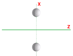
Figure 7: Two steady sources with a distance between them of $2d$ in the $x-$direction.

7 Two Sources

7.1 Two Sources at rest

For emission from two steady sources in Heavy-Ion Collisions, two-photon correlations were studied in Ref. [38]. Here we use our represented method. We assume that the two source system is symmetric, i.e. both positions of the sources are placed symmetrically and also their normal vectors, $\hat{\sigma}^{\mu}$, are the same, Fig. 7. If the normal were $\hat{\sigma}^{\mu}=(1,0,0,0)$, then the invariant scalar $k^{\mu}\,\hat{\sigma}_{\mu}=k^{0}$; it has been mentioned already that we actually do not need this additional requirement to illustrate the correlation function, which would arise from an idealized symmetric system. In case of two symmetric sources at rest ($\gamma_{s}=1$) the source function is (for stars we can savely assume $H_{1}\left(t\right)=H_{2}\left(t\right)$):

$$S(x,k) = \sum\limits_{s=1,2}\,S_{s}\left(x,k\right)$$ (90)

$$= (k^{\mu}\hat{\sigma}_{\mu})H\left(t\right)\,\sum\limits_{s=1,2}\frac{G_{s}\left(x,y,z\right)\,}{C_{\gamma}}\,\exp\left[-\frac{k\cdot u_{s}}{T_{s}}\right]\,,$$

while the function $J$ in the Jüttner approximation is

$$J_{(\pm)}(k,q) = \sum\limits_{s=1,2}\exp\left[\mp\frac{\kappa\cdot u_{s}}{2T_{s}}\right]\,\exp(iqx_{s})\int_{S}d^{4}x\ S_{s}(x,k)\,\exp(iqx)\,,$$ (91)

where $x_{s}$ is the position of the center of the source, and the spatial integrals run separately for each of the identical sources, i.e. we assume stars with identical density profiles, but with different temperatures, $T_{s}$.

In case of steady sources $u^{\mu}_{s}=(1,0,0,0)$, and the spatial integral for one source is the same as for a single source. Thus,

$$\int d^{4}x\,S\left((x,k\right) = \sum\limits_{s=1,2}\int_{s}d^{4}x\,S_{s}\left(x,k\right)$$ (92)

$$= \left(2\pi R^{2}\right)\,(k^{\mu}\hat{\sigma}_{\mu})\sum\limits_{s=1,2}\,\frac{D}{C_{\gamma}}\exp\left(-\frac{E_{k}}{T_{s}}\right),$$

and

$$J_{(\pm)}(k,q) = \sum\limits_{s=1,2}\exp\left[\mp\frac{{\kappa}^{0}}{2T_{s}}\right]\,\exp(iqx_{s})\int_{S}d^{4}x\,S_{s}\left(x,k\right)\,\exp(iqx)$$ (93)

$$= \left(2\pi R^{2}\right)\,(k^{\mu}\hat{\sigma}_{\mu})\,\exp\left(-\frac{R^{2}}{2}\,q^{2}\right)$$

$$\times\sum\limits_{s=1,2}\frac{D}{C_{\gamma}}\exp\left(-\frac{E_{k}}{T_{s}}\right)\exp\left[\mp\frac{{\kappa}^{0}}{2T_{s}}\right]\,\exp(i\,q^{0}\,x^{0}_{s})\exp(-i\mbox{\boldmath$q$}\cdot\mbox{\boldmath$x$}_{s})\,.$$

In the $J(k,q)_{(+)}J(k,-q)_{(-)}$ product the terms $\exp[\pm{\kappa}^{0}/(2T_{s})]$ cancel each other. Both $J(k,q)_{(+)}$ and $J(k,-q)_{(-)}$ includes a sum $[\exp(i\mbox{\boldmath$q$}\cdot\mbox{\boldmath$x$}_{s})+\exp(-i\mbox{\boldmath$q$}\cdot\mbox{\boldmath$x$}_{s})]$, and their product leads to a factor $2[1+\cos(2\mbox{\boldmath$q$}\cdot\mbox{\boldmath$x$}_{s})]$. Consequently, if the two sources have the same parameter, just different locations, $x_{1}=-x_{2}$ (see Fig.84) then

$$C(k,q)=1+\frac{1}{2}\exp(-R^{2}q^{2})[1+\cos(2\mbox{\boldmath$q$}\cdot\mbox{\boldmath$x$}_{s})].$$ (94)

Like above in case of one source, one may compare the correlation function for binaries in (94) with the previous result Eq. (42). The difference between these both results is caused by the Gaussian source function in (57) which is used in order to obtain (94), while in (42) the Einstein-Hopf model for the thermal radiation source has been applied.

This result agrees with Ref. [38] (Section 9.1 on p.41 ibid.), and in the limit of $\mbox{\boldmath$x$}_{s}=0$ it returns the single source result, Eq. (84). If the distance of the two sources is $2d$, i.e. $x_{1}=d$ and $x_{2}=-d$, then $2\mbox{\boldmath$q$}\cdot\mbox{\boldmath$x$}_{s}=2q_{x}\,d$, thus the modification appears in the $q_{x}$-direction only. In the other directions, $q_{y}$, the single source result (84) is returned. For distances under $4R$ the zero-points are artificial because the stars will overlap.

7.1.1 Sources with varying distances

Eq. (94) is valid when the two stars are close to each other relative to us. That means, they have just past each other in the orthogonal plane. We parametrize the distance between the stars, $\mbox{\boldmath$x$}_{s}$ with a time component, $x_{s}\rightarrow x_{s}(t)$.

Figure 8: Four diagrams of the correlation function in Eq. (97). The two figures at the top show the oscillation of the correlation function over periods $1\,{\rm a.u.}$ and $25\,{\rm a.u.}$ respectively. The two figures at the bottom show the reduction of the oscillation. The x-axis is to get a perspective of the time scales. The parameters are: $\textit{R}=1.2\times 10^{9}$m, $\textit{k}=7.85\times 10^{6}$m^-1, $\textit{L}=4.14\times 10^{16}{\rm m}$, $d=1m$, major axis A is $1\,{\rm a.u.}$, orbital period 0.7 year.

Assuming the stars rotate each other in circular orbits, the distance $\mbox{\boldmath$x$}_{s}\left(t\right)$ on the major axis is given by

$$x_{s}(t)=A\sin(\frac{2\pi}{\mathcal{T}}t+\Phi),$$ (95)

where A is the maximum distance of the major axis, and $\mathcal{T}$ is the total orbital period. $\Phi$ is a phase shift to be adjusted such that when $t=0$, the two stars have just past each other, $x_{s}(0)=2R$, where R is the radius of the star. Our simple model is not applicable when one star is behind the other, shadowing the light from one of the stars. This will give us the possibility to have the detector distance fixed, and Eq. (94) will depend on time. For two sun-like stars, with A=25 a.u., G is Newton’s gravitational constant, the period is given by Kepler’s third law:

$$\mathcal{T}=2\pi\sqrt{\frac{A^{3}}{G(M_{A}+M_{B})}}=2.7\times 10^{9}\,s\ \simeq 85\,y,$$ (96)

where $M_{A}$ and $M_{B}$ are the masses of the two stars. Hence, Eq. (94) becomes

$$C(q,t) = 1+\frac{1}{2}e^{-R^{2}q^{2}}[1+\cos(2qx_{s}(t))]$$ (97)

$$= 1+\frac{1}{2}e^{-R^{2}q^{2}}[1+\cos(2qA\sin(\frac{2\pi}{\mathcal{T}}t+\Phi))]\,.$$

At $d=1m$ there is a rapid oscillation, but there is a rather special behaviour when the sign of the gradient of the sine changes. Four figures for two different orbital periods (and hence major axis) are plotted in Fig. 8, one for $A=1\,a.u.$, and the second for $A=25\,a.u.$ respectively.

As seen in Fig. 8 there are rapid oscillations, but there is an interesting effect appearing during a period of rotation. During the turning points of the sine function the correlation function get a reduction in the oscillation. The reduction appears when the stars reaches their maximum separation on the axis parallel to the rotation. If the stars are rotating in elliptical orbits, the reduction will be different depending if they are at a maximum, or minimum separation. Finally, the correlation function over a longer period and over different distances is shown in Fig. 9.

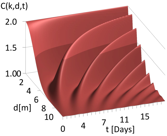
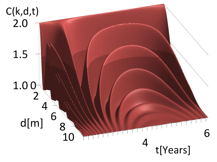
Figure 9: The correlation Eq. (94) plotted against time $t$, and detector distance $d$, with the corresponding parameters, distance to system $L=4.14\cdot 10^{16}m$, wave-vector $k=7.85\cdot 10^{6}$, phase shift $\Phi=1.64\cdot 10^{-4}$, max major axis amplitude $A=25AU$, mean-radius of stars $R=1.20\cdot 10^{9}m$. Second picture is over a turning point.

7.1.2 Sources with elliptical orbits

A binary system with an elliptical orbit, Fig. 10, is characterised by the eccentricity $e$. This will effect the relative velocities they pass each other as seen from our point of view, if they are transiting each other when they are closest, or furthest away. In this ideal scenario we will lie on the major axis. Then the stars will move faster when they are closest to each other. If we imagine that the two stars pass each other when they have their furthest and closest distance, to first approximation then they should show two slightly different correlation functions after the crossing because of the different velocities. We can consider the difference (differential HBT method),

$$\delta C(k,q,t)=\frac{1}{2}\left(\cos\left(2q\frac{A}{1{+}e}\sin\left(\frac{2\pi}{\mathcal{T}_{1}}t+\Phi_{1}\right)\right)-\cos\left(2q\frac{A}{1{-}e}\sin\left(\frac{2\pi}{\mathcal{T}_{2}}t+\Phi_{2}\right)\right)\right)e^{-R^{2}q^{2}},$$ (98)

and this function vanishes for $\epsilon=0$ when they are orbiting in perfect circles; here $T_{1/2}$ is the orbital period for the furthest and closest distances, and $\Phi_{1/2}$ the two phase shits respectively and the dependence on the distance with the eccentricity is given by $r_{max}=A(1+\epsilon)$ and $r_{min}=A(1-\epsilon)$ [41]. The period are based on circular motion at these distances, so they are only an approximation for a short time.

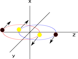
Figure 10: Two Stars orbiting around a common center-of-mass in an elliptical orbit.

Eq. (98) has a very particular shape that can be seen in Fig. 11a and Fig. 11b. It will show its effect in just a couple of days. The closer the system is in a circular orbit the longer their correlation functions stays in phase. This can be a method of assisting in determination of the orbital period, velocity and eccentricity in case these two stars can’t be resolved separately.

Figure 11: The differential HBT correlator as given by Eq. (98). The parameter are the following: Left pannel: $e=0.01$. Right pannel: $e=0.5$. Furthermore, orbital period ${\cal T}=1\,{\rm year}$, stellar mean-radius $\textit{R}=1.2\cdot 10^{9}$m, wave-number $\textit{k}=7.85\cdot 10^{6}$m^-1, distance between stars and detectors $\textit{L}=4.14\cdot 10^{16}{\rm m}$, distance of both detectors $d_{AB}=1m$, $A=1\,a.u.$.

7.2 Two sources in motion

We study the system the same way as before, but now we use the present method. The two sources are moving in opposite directions, so that $u_{s}=u_{1}$ or $u_{2}$ where $u_{1}^{\mu}=\gamma_{s}\left(1,\mbox{\boldmath$v$}_{1}\right)$, $u_{2}=\bar{u}_{s}^{\mu}=(\gamma_{s},\gamma_{s}(-\mbox{\boldmath$v$}_{1}))$, and $\mbox{\boldmath$u$}_{s}\equiv\gamma_{s}\,\mbox{\boldmath$v$}_{s}$, so that $\mbox{\boldmath$u$}_{1}=-\mbox{\boldmath$u$}_{2}$, see Fig. 12. Similarly, $x_{s}=x_{1}$ or $x_{2}$ where $x_{s}^{\mu}=(t_{s},\mbox{\boldmath$x$}_{s})$, $\bar{x}_{s}^{\mu}=(t_{s},-\mbox{\boldmath$x$}_{s})$, and $\mbox{\boldmath$x$}_{1}=-\mbox{\boldmath$x$}_{2}$. We assume again $\hat{\sigma}^{\mu}=(1,0,0,0)$ for the normal of hypersurface, and $t_{1}=t_{2}$. For binary stars the change of the velocity, and position due to the rotation (which is having a frequency of the order of 1/day) can be considered as quasi-static, so the two-photon correlation is not effected by this change. If we have several sources then the source function is

$$S\left(x,k\right) = \sum\limits_{s=1,2}S_{s}\left(x,k\right)=(k^{\mu}\,\hat{\sigma}_{\mu})H\left(t\right)\,\sum\limits_{s=1,2}\frac{G_{s}(x,y,z)}{C_{\gamma}}\,\exp\left[-\frac{k\cdot u_{s}}{T_{s}}\right]\,,$$ (99)

while the $J$ function is

$$J(k,q)_{(\pm)} = \sum\limits_{s=1,2}\exp\left[\mp\frac{\kappa\cdot u_{s}}{2T_{s}}\right]\exp(iqx_{s})\int_{S}d^{4}x\,S_{s}(x,k)\,\exp(iqx)\,,$$ (100)

where $x_{s}$ is the 4-position of the center of source $s$, and the spatial integrals run separately for each of the identical sources, i.e. we assume stars with identical density profiles, but with different velocities, $u_{s}$ and temperatures, $T_{s}$.

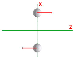
Figure 12: (color online) Two moving sources in the reaction ($[x-z]$) plane with a distance between them of $2d$ in the $x-$direction. The sources are moving in the directions indicated by the (red) arrows.

The integral for one source is very similar as for the case of one single source. Thus,

$$\int d^{4}x\,S\left(x,k\right)=\sum\limits_{s=1,2}\int_{S}d^{4}x\,S_{s}\left(x,k\right)$$ (101)

$$= (k^{\mu}\,\hat{\sigma}_{\mu})\,\left(2\pi R^{2}\right)\gamma_{s}\,\frac{D}{C_{\gamma}}\exp\left(-\frac{k^{0}\gamma_{s}}{T_{s}}\right)\left[\exp\left(\frac{\mbox{\boldmath$k$}\cdot\mbox{\boldmath$u$}_{s}}{T_{s}}\right)+\exp\left(-\frac{\mbox{\boldmath$k$}\cdot\mbox{\boldmath$u$}_{s}}{T_{s}}\right)\right].$$

This result returns Eq. (92) if $u^{\mu}_{s}=(1,0,0,0)$. The function $J_{(\pm)}(k,q)$ becomes

$$J_{(\pm)}(k,q) = \sum\limits_{s=1,2}\exp\left[\mp\frac{\kappa\cdot u_{s}}{2T_{s}}\right]\,\exp(iqx_{s})\int_{S}d^{4}x\,S_{s}(x,k)\,\exp(iqx)$$

$$=(k^{\mu}\,\hat{\sigma}_{\mu}) \!\!\!\!\!\!\!\!\!\!\!\left(2\pi R^{2}\right)\exp\left(-\frac{R^{2}q^{2}}{2}\right)\sum\limits_{s=1,2}\frac{\gamma_{s}\,D}{C_{s}}\exp\left[-\frac{k\cdot u_{s}}{T_{s}}\right]\exp\left[\mp\frac{\kappa\cdot u_{s}}{2T_{s}}\right]\,\exp(iqx_{s})$$

$$=(k^{\mu}\,\hat{\sigma}_{\mu}) \!\!\!\!\!\!\!\!\!\!\!\left(2\pi R^{2}\right)\exp\left(-\frac{R^{2}}{2}q^{2}\right)\frac{\gamma_{s}\,D}{C_{s}}\exp\left[\mp\frac{k^{0}\gamma_{s}}{T_{s}}\right]\exp\left[\mp\frac{{\kappa}^{0}}{2}\frac{\gamma_{s}}{T_{s}}\right]\exp(iq^{0}x_{s}^{0})$$

$$\times\left[\exp\left[\frac{\mbox{\boldmath$k$}\cdot\mbox{\boldmath$u$}_{s}}{T_{s}}\right]\exp\left[\pm\frac{\mbox{\boldmath$\kappa$}\cdot\mbox{\boldmath$u$}_{s}}{2T_{s}}\right]\exp(-i\mbox{\boldmath$q$}\cdot\mbox{\boldmath$x$}_{s})+\exp\left[-\frac{\mbox{\boldmath$k$}\cdot\mbox{\boldmath$u$}_{s}}{T_{s}}\right]\exp\left[\mp\frac{\mbox{\boldmath$\kappa$}\cdot\mbox{\boldmath$u$}_{s}}{2T_{s}}\right]\exp(i\mbox{\boldmath$q$}\cdot\mbox{\boldmath$x$}_{s})\right],$$

where the factor $\exp(iq^{0}x_{s}^{0})$ can be dropped if the time distribution is simultaneous for the two sources, because then $x_{s}^{0}=0$. We have again approximated $\kappa$ as a constant, $\kappa=k\Theta$. This allows us treat $\kappa$ as a constant of the integrals. This returns Eq. (93) if $u^{\mu}_{s}=(1,0,0,0)$. Now we can divide the two-photon correlation with the square of the single photon distribution

$$\frac{Re\,[J_{(+)}(k,q)\,J_{(-)}(k,-q)]}{\left|\int d^{4}x\,S(x,k)\right|^{2}} = \exp(-R^{2}q^{2})\frac{\cosh\left(\frac{\displaystyle 2\,\mbox{\boldmath$k$}\cdot\mbox{\boldmath$u$}_{s}}{\displaystyle T_{s}}\right)+\cosh\left(\frac{\displaystyle\mbox{\boldmath$\kappa$}\cdot\mbox{\boldmath$u$}_{s}}{\displaystyle T_{s}}\right)\cos(2\,\mbox{\boldmath$q$}\cdot\mbox{\boldmath$x$}_{s})}{\cosh\left(\frac{\displaystyle 2\,\mbox{\boldmath$k$}\cdot\mbox{\boldmath$u$}_{s}}{\displaystyle T_{s}}\right)+1}\,.$$

Consequently, if the two sources have the same parameter, just opposite locations with respect to the center, and opposite velocities, then the correlation function is

$$C(k,q) = 1+\exp(-R^{2}q^{2})\frac{\cosh\left(\frac{\displaystyle 2\,\mbox{\boldmath$k$}\cdot\mbox{\boldmath$u$}_{s}}{\displaystyle T_{s}}\right)+\cosh\left(\frac{\displaystyle\mbox{\boldmath$\kappa$}\cdot\mbox{\boldmath$u$}_{s}}{\displaystyle T_{s}}\right)\cos(2\,\mbox{\boldmath$q$}\cdot\mbox{\boldmath$x$}_{s})}{\cosh\left(\frac{\displaystyle 2\,\mbox{\boldmath$k$}\cdot\mbox{\boldmath$u$}_{s}}{\displaystyle T_{s}}\right)+1}\,.$$ (104)

This expression returns Eq. (94) if $u^{\mu}_{s}=(1,0,0,0)$, and $C(k,q)=2$ if $q=0$.

7.3 Two simplest configurations

We will now consider two configurations I and II, where in case I the orbital, $[x,y]$ plane is perpendicular to the direction of the observer, $[z]$, on the Earth, and II where the Earth is in the plane of rotation, in direction $z$. We assume furthermore that the two stars of the binary have the same mass, temperature and their orbits are identical circular orbits. This is a highly simplified configuration compared to the general configuration in Fig. 1.

7.3.1 I - Orbital plane is orthogonal to the direction of the Earth

This configuration is shown in Fig. 13.

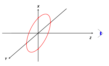
Figure 13: The trajectory of the Binary system is in the $[x,y]$-plane, the observer is in the orthogonal, $z$-direction to the plane. The $z$-axis is the rotation axis.

Let the angular speed of rotation be $\omega$, and $k\gg q$, $\mbox{\boldmath$k$}=(0,0,k_{z})$ but the small differences in $q$ can be measured. We need to determine the source parameter, $\mbox{\boldmath$u$}_{s}$ and $\mbox{\boldmath$x$}_{s}$. If the radius of the orbit is $A$ and the angular velocity of the rotation is $\omega$ then $u_{s}=\omega A$ and $x_{s}=d=A$. The two stars are opposite to each other so that $\mbox{\boldmath$u$}_{A}=\mbox{\boldmath$u$}_{s}$, $\mbox{\boldmath$u$}_{B}=-\mbox{\boldmath$u$}_{A}$, $\mbox{\boldmath$x$}_{B}=-\mbox{\boldmath$x$}_{A}$. These vectors are time dependent: So, for anti-clockwise rotation $\mbox{\boldmath$x$}_{s}=x_{s}\,(\cos(\omega t),\sin(\omega t),0)$, and $\mbox{\boldmath$u$}_{s}=u_{s}\,(-\sin(\omega t),\cos(\omega t),0)$.

In case I, the vector $k$ is orthogonal to both $\mbox{\boldmath$u$}_{A}$ and $\mbox{\boldmath$u$}_{B}$ all the time, so we can have a $z$ directed $k$ only, and so $(\mbox{\boldmath$k$}\cdot\mbox{\boldmath$u$}_{s})$ vanishes. The products $(\mbox{\boldmath$q$}\cdot\mbox{\boldmath$x$}_{s})$ and $(\mbox{\boldmath$\kappa$}\cdot\mbox{\boldmath$u$}_{s})$ for $z$ directed $q$ vanish so

$$C(k_{z},q_{z})=1+\exp(-R^{2}q^{2}_{z})\ .$$ (105)

Usually $R\ll A$, therefore $C(k_{z},q_{z})\approx 2$ for astronomical configurations, and the dependence on the much larger $A$ leads to stronger variation at smaller $q$ values:

$$C(k_{z},q_{x})\! = \!1{+}\frac{1}{2}\exp(-R^{2}q^{2}_{x})\left[1+\cos\left(2q_{x}A\cos(\omega t)\right)\cosh\left(\frac{{-}\kappa_{x}\omega A\sin(\omega t)}{T_{s}}\right)\right],$$

$$C(k_{z},q_{y})\! = \!1{+}\frac{1}{2}\exp(-R^{2}q^{2}_{y})\left[1+\cos\left(2q_{y}A\sin(\omega t)\right)\cosh\left(\frac{\kappa_{y}\omega A\cos(\omega t)}{T_{s}}\right)\right].$$ (106)

Here we assumed that the orbital velocity of the binary star components is non-relativistic, so we can neglect the relativistic $\gamma$ factor. $\kappa_{x}$ and $\kappa_{y}$ are respectively the mean angular size in x, and y direction. For a symmetric source they are both $\kappa_{x}=\kappa_{y}=k\frac{2R}{L}=k\Theta$.

As $R\ll A$ the leading exponential term tends to $1$ for small and intermediate $q_{x}$ or $q_{y}$ values. At the same time at $q_{x}=q_{y}=0$ both the $\cos$ and $\cosh$ terms tend to $1$, so the value of the correlation function is $2$. The $\cos$ terms drop to zero when $q_{x}=\pi/[2A\cos(\omega t)]$ or $q_{y}=\pi/[2A\sin(\omega t)]$. These terms may drop much faster than the leading exponential term as $A\gg R$, and show a rather special $t$ depencence due to the orbital rotation.

The arguments in the $\cosh$ terms are of the order $\approx 10^{-8}$ for a binary configuration. Same with the two stars orbiting with a distance $1\,a.u.$. This is no surprise because the extra terms are coming from the velocity dependence of the emission function through Jüttner distribution. The velocity is given by $\omega A\approx 400\frac{km}{s}$. Thus Eq. (106) effectively goes back to the result presented earlier when the velocities of the sources where not explicitly accounted for.

Eq. (106) goes like the earlier result Eq. (97), as a consequence of the velocity-dependent part of the correlation function going to unity.

7.3.2 II - The direction of the Earth falls in the orbital plane

This configuration can in principle occur in two ways, the $z$-axis is spanning the distance between the center of the Binary and the observer on the Earth, and the plane of rotation of the binary can either be the $[x,z]$-plane or the $[y,z]$-plane, see Fig. 14 and Fig. 15.

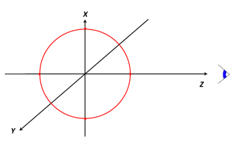
Figure 14: The trajectory of the Binary system is in the $[x,z]$-plane, the observer is in the plane in the $z$-direction.

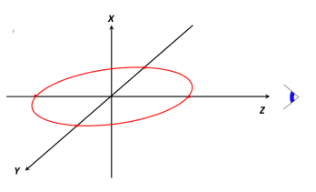
Figure 15: The trajectory of the Binary system is in the $[y,z]$-plane, the observer is in the plane in the $z$-direction.

We can freely choose the direction of the $x$ and $y$ axes, so we chose the configuration so that the rotation plane of the Binary is the $[x,z]$-plane. Consequently, with this choice neither the distance between the two starts of the binary nor their velocity will have any $y$-component, see Fig. 14. Thus in case II the relation between $u_{s}$ and $x_{s}$ are the same, but now the anti-clockwise rotation is in the [x,z] plane, $\mbox{\boldmath$x_{s}$}=x_{s}\,(\cos(\omega t),0,\sin(\omega t))$ and $\mbox{\boldmath$u_{s}$}=u_{s}(-\sin\omega t,0,\cos(\omega t))$.

The decomposition of the correlation function, Eq. (104) now becomes:

$$C(k_{z},q_{x}) = 1+\exp(-R^{2}q^{2}_{x})\frac{\cosh\left(\frac{2k_{z}\omega A\cos(\omega t)}{T_{s}}\right)+\cosh\left(\frac{-\kappa_{x}\omega A\sin(\omega t)}{T_{s}}\right)\cos(2q_{x}A\cos(\omega t))}{\cosh\left(\frac{2k_{z}\omega A\cos(\omega t)}{T_{s}}\right)+1}\,,$$

$$C(k_{z},q_{y}) = 1+\exp(-R^{2}q^{2}_{y}),$$

$$C(k_{z},q_{z}) = 1+\exp(-R^{2}q^{2}_{z})\frac{\cosh\left(\frac{2k_{z}\omega A\cos(\omega t)}{T_{s}}\right)+\cosh\left(\frac{\kappa_{z}\omega A\cos(\omega t)}{T_{s}}\right)\cos(2q_{z}A\sin(\omega t))}{\cosh\left(\frac{2k_{z}\omega A\cos(\omega t)}{T_{s}}\right)+1}\,.$$

Just as in the previous case, we have assumed that the orbital velocity of the binary star components is non-relativistic, so we can neglect the relativistic $\gamma$ factor. Also as we have seen the term $\cosh(\kappa_{\mu}u^{\mu})\approx 1$, and the argument in $\cosh(k_{z}u_{z})$ is of order $\approx 10^{-4}$. This is also $1$ for an ordinary binary system. Even for the fastest binary observed with a period of 5 minutes the contribution is only of $\approx 1.004$ [42].

8 Summary and Outlook

Our investigation starts with a reconsideration of the classical HBT effect, both in terms of classical electrodynamics and quantum electrodynamics. Within a simple model for the thermal radiation field we have determined the correlation function for stars at rest in Eq. (17), and we have explained how one may deduce the diameter of stars from this correlator. Afterwards, the correlation function for binary systems has been determined in Eq. (42) for comparsion with a modified HBT approach used in heavy-ion collisions. Another aspect which has carefully to be treated concerns the two-photon wavefunctions, which differ in case of stars and heavy-ion collisions (HIC), because of the different geometrical limits of detector distances and radial diamater of the thermal sources, i.e. either stars or hadronic fireballs.

Afterwards, inspired by recent developments with HBT analyses in heavy-ion collisions taking the relative velocity of the sources into account, we have tried to modify the HBT approach used in heavy-ion collisions to the case of binary star systems. Especially, we we have considered the differential HBT approach as it is in use for analyzing the hadronic fireballs created in heavy-ion collision experiments.

Since the fireball in heavy-ion collisions expands rapidly in space and time, the correlation function in HIC is determined by covariant integrals over the four-dimensional space-time. On the other side, stars emit permanently thermal radiation and ther stellar radii remain constant. Furthermore, the opacity of stars is usually so extremely high, that the photons only originate from the two-dimensional surface of the stars nstead from the entire three-dimensional volume of the stars. Accordingly, the HBT approach used in HIC has to be modified for the case of stars by simplifiying the four-dimensional integrals itno two-dimensional integrals.

A further key-point in order to determine the correlator regards the emission function which determines the number of photons emitted into a phase-space element. Furthermore, it has been shown that the Jüttner-distribution, frequently used in HIC, is also a good approximation for stars. Then the new approach has been applied in order to determine the correlator for stars at rest in Eq. (84) and for stars in motion in Eq. (89), While an exact agreement between the classical approach and the modified HIC approach cannot be expected because of the different descriptions for the thermal radiation field, we have shown that the result in (84) corresponds to the previuos result in Eq. (17),

Then we have determined the correlation function for binary stars at rest to each other in Eq. (94) and for the case of binary stars in motion in Eq. (104). Like in case of one star, we have shown that the result in Eq. (94) obtained from the modified HIC approach corresponds to the expression in Eq. (42) which was obtained from the classical HBT approach.

The first results of our approach have shown that the dependence on velocities do not influence the correlation function for normal binary stars, as one expected. But the rather specific oscillation dependence of the correlation function during a period of rotation is a characteristic sign of binary systems, and can help to determine some parameters of the orbits when the stars are not optically resolved. This has been elucidated by the difference of the two correlators of a binary system (differential HBT approach) in Eq. (98).

It has been outlined that due to the restriction of real experiments being bounded on Earth limits the possibility of fully exploiting the correlation function compared to heavy-ion collisions. Our model assumes a thermally equilibrium symmetric sources, while more exotic objects could in principle also be investigated within the approach presented.

9 Acknowledgements

One of the authors (S.Z.) thanks for the pleasant hospitality of the Physics Department at Bergen University (BCPL, Bergen/Norway). He also acknowledges for kind support from Professor Joerg Aichelin (Subatech, Nantes/France).

References

- [1] R. Hanbury Brown, R.Q. Twiss, Nature 177, 27 (1956).
- [2] R. Hanbury Brown, R.Q. Twiss, Nature 178, 1046 (1956).
- [3] G. Goldhaber, S. Goldhaber, W. Lee and A. Pais, Phys. Rev. 120, 300 (1960).
- [4] H. Boggild et al., NA44 collaboration, Phys. Lett. B 302, 510 (1993); Phys. Lett. B 349, 386 (1995).
- [5] D. Miskowiec et al., E877 collaboration, Nucl. Phys. A 610, 237c (1996).
- [6] M.A. Lisa, N.N. Ajitanand, J.M. Alexander, et al., Phys. Lett. B 496, 1 (2000); M.A. Lisa, U. Heinz, U.A. Wiedemann, Phys. Lett. B 489, 287 (2000); E. Mount, G. Graef, M. Mitrovski, M. Bleicher, M.A. Lisa, Phys. Rev. C 84, 014908 (2011).
- [7] M. Lisa, S. Pratt, R. Soltz, U. Wiedemann, Ann. Rev. Nucl. Part. Sci. 55 357 (2005); arXiv:nucl-ex/0505014v2.
- [8] S. Pratt, Phys. Rev. Lett. 53, 1219 (1984).
- [9] L.P. Csernai, V.K. Magas, H. Stöcker, and D.D. Strottman, Phys. Rev. C 84, 024914 (2011).
- [10] L.P. Csernai, D.D. Strottman and Cs. Anderlik, Phys. Rev. C 85, 054901 (2012).
- [11] L.P. Csernai, S. Velle, Int. J. Mod. Phys. E 23, 1450043 (2014).
- [12] L.P. Csernai, S. Velle and D.J. Wang, Phys. Rev. C 89, 034916 (2014).
- [13] L.P. Csernai, S. Velle and D.J. Wang, Nucl. Phys. A 931, 1056 (2014).
-
[14]
USNO, NAVY: The Washington Double Star Catalog (2012)
http://www.usno.navy.mil/USNO/astrometry/optical-IR-prod/wds/WDS - [15] R. Hanbury Brown, R.Q. Twiss, Phil. Mag. 45, 663 (1954).
- [16] R.J. Glauber, Phys. Rev. 130, 2529 (1963).
- [17] R.J. Glauber, Phys. Rev. Lett. 10, 84 (1963).
- [18] R.J. Glauber, Phys. Rev. 131, 2766 (1963).
- [19] J.D. Jackson, Classical Electrodynamics, John Wiley and Sons, 3. Ed., (1998).
- [20] A. Einstein and L. Hopf, Ann. d. Phys. 33, 1105 (1910).
- [21] M.O. Scully, M.S. Zubairy, Quantum Optics, Cambridge University Press, (1997).
- [22] Thomas J. Humanic, Int. J. Mod. Phys. E 15, 197 (2006).
- [23] U. Heinz, B.V. Jacak, Ann. Rev. Nucl. Part. Sci. 49 529 (1999).
- [24] B. Saleh, Photoelectron Statistics, Springer, Berlin, 1978.
- [25] H. Chen, T. Peng, S. Karmakar, Z. Xie and Y. Shih, Phys. Rev. A 84, 033835 (2011).
- [26] A.I. Akhiezer, W.B. Berestezki, Quantum Electrodynamics, New York, Consultants Bureau 1957, 2. Ed., Wiley (1965).
- [27] A.S. Davydov, Qantum Mechanics, Headington Hill Hall, Oxford, England, 2. Ed., Pergamon Press (1976).
- [28] L. Landau and R. Peierls, Z. Phys. 69, 56 (1931).
- [29] E.C.G. Sudarshan and T. Rothman, Am. J. Phys. 59, 592 (1991).
- [30] I. Bialynicki-Birula, Acta Physica Polonica A 86, 97 (1994); Photon Wave Function in E. Wolf Ed., Progress in Optics XXXVI, Elsevier, Amsterdam (1996).
- [31] B.J. Smith and M.G. Raymer, New J. Phys. 9, 414 (2007).
- [32] W. Florkowski: Phenomenology of Ultra-relativistic heavy-Ion Collisions, World Scientific Publishing Co., Singapore (2010).
- [33] D. Miskowiec, et al., E877 Collaboration, Nucl. Phys. A 590, 557c (1995).
- [34] B. Cameron Reed, J. Roy Astron. Soc. Can., Vol. 87, 123 (1993).
- [35] S. Jordan, The Gaia Project - technique, performance and status. Astron. Nachr. 329 (2008) 875; arXiv:0811.2345v1.
- [36] L.P. Csernai: Introduction to relativistic heavy ion collisions, Wiley, Chichester (1994).
- [37] F. Cooper, G. Frye, Phys. Rev. D 10, 186 (1974).
- [38] T. Csörgő, Heavy Ion Phys. 15, 1-80, (2002); arXiv: hep-ph/0001233v3.
- [39] M. Csanád, M. Vargyas, Eur. Phys. J. A 44, 473 (2010).
- [40] I.S. Gradshteyn and I.M. Ryzhik: Table of integrals, series and products, Academic Press (1965).
- [41] E. Lillestøl, O. Hunderi, R. Lien, Generell Fysikk for Universiteter og hogskoler, Bind 2 Unversitetsforlaget (2006).
- [42] S.C. C. Barros et. al ULTRACAM photometry of the ultracompact binaries V407 Vul and HM Cnc, Monthly Notices of the Royal Astronomical Society, 374, 1334 (2007).