Generalized Second Law of Thermodynamics in $f(T,T_{G})$ gravity

Abstract

An equilibrium picture of thermodynamics is discussed at the apparent horizon of FRW universe in $f(T,T_{G})$ gravity, where $T$ represents the torsion invariant and $T_{G}$ is the teleparallel equivalent of the Gauss-Bonnet term. It is found that one can translate the Friedmann equations to the standard form of first law of thermodynamics. We discuss GSLT in the locality of assumption that temperature of matter inside the horizon is similar to that of horizon. Finally, we consider particular models in this theory and generate constraints on the coupling parameter for the validity of GSLT in terms of recent cosmic parameters and power law solutions.

Keywords: $f(T,T_{G})$ theory; Dark Energy; Thermodynamics.
PACS: 04.50.Kd; 95.36.+x; 97.60.Lf; 04.70.Df.

1 Introduction

The discovery of black hole (BH) thermodynamics suggest that there is a fundamental connection between relativistic gravity and thermodynamics laws, however people have been trying to find a significant way to develop such connection [1]. BH acts as a thermodynamic system with temperature being related to surface gravity and entropy with horizon area [2]. Jacobson [3] unveiled the issue of relating BH thermodynamics to the Einstein gravity and derived Einstein field equations in local Rindler spacetime using the entropy $S=A/4G$ and Clausius relation $TdS=\delta{Q}$. Frolov and Kofman [4] showed that for the flat quasi de-Sitter geometry of inflationary universe, Friedmann equations can result from $dE=TdS$ for slowly rolling scalar field. In [5], Padmanabhan explored such connection in case of spherically symmetric BHs and showed that field equations can be stated in the form $dE+PdV=TdS$. This study is further extended to generic static spacetimes in Lanczos-Lovelock gravity and shown that the near-horizon field equations again represent a thermodynamic identity in all these models [6].

Cai and Kim [7] showed that Friedmann equations with any spatial curvature can be derived from the Clausius relation $TdS=\delta{Q}$. The relation between gravity and thermodynamics has also been tested in Einstein as well as Gauss-Bonnet and Lovelock gravities. Cai and Cao [8] showed that Friedmann equations in braneworld scenario can be cast to the form of first law of thermodynamics at the apparent horizon. This work is also extended in the framework of warped DGP braneworld [9] and Gauss-Bonnet Braneworld [10]. Akbar and Cai [11] found that formulation of thermodynamic laws in $f(R)$ and scalar tenser gravities is not trivial when compared to Einstein gravity and Clausius relation is to be modified. In this perspective, Eling et al. [12] studied the thermodynamic laws in $f(R)$ gravity and remarked that non-equilibrium description of thermodynamics needed, whereby the Clausius relation is modified to the form $\delta{Q}=T(dS+d_{\jmath}{S})$, where $d_{\jmath}{S}$ is the additional entropy term. Cai and Cao [13] found that in scalar tensor theories thermodynamics associated with the apparent horizon of the FRW universe results in non-equilibrium description which modifies the standard Clausius relation. The thermodynamics properties have been discussed in various modified theories [14]-[20].

The development of cosmology and gravitation can be seen as one of the scientific triumphs of the twentieth century. In current situation modified theories of gravity have been appeared as significant tool to discuss various cosmic issues [21]. The introduction of non-minimal coupling between matter and curvature in the context of modified theories has become a center of interest for the researchers [22]. Another important and conceptually rich class consists of gravitational modifications involving torsion description of gravity. It is interesting to mention here that teleparallel equivalent of GR has been constructed by Einstein himself by including torsionless Levi-Civita connection instead of curvatureless Weitzenb ck connection and the vierbein as the fundamental ingredient for the theory [23]. Harko et al. [24] constructed a more general type of $f(T)$ gravity by introducing a non-minimal interaction of torsion with matter in the Lagrangian density. We [25, 26] have discussed the validity of energy bounds and GSLT for specific models and find the feasible constraints on the involved free parameters. Kofinas and Saridakis [27] proposed a novel theory namely $f(T_{G})$ gravity and then its generalized form $f(T,T_{G})$ gravity and they also discussed its cosmological significance. Recently, we have discussed the energy condition bounds in this modified gravity and tested two well known models [28] which are proposed in [27].

In this study, we are interested to explore laws of thermodynamics in $f(T,T_{G})$ gravity which is a more generic modified theory involving torsion and Gauss-Bonnet contributions [27]. In previous studies, we have explored the issue of equilibrium thermodynamics in $f(R,T)$ [29], $f(R,L_{m})$ [30] and $f(R,T,R_{\mu\nu}T^{\mu\nu})$ [31] theories of gravity. We find that equilibrium picture of thermodynamics in such theories needs more study to follow. However, in this paper we find that one can develop the equilibrium picture of thermodynamics in generic modified theory models which involve contribution from torsion scalar. The paper has the following format: In section 2, we present the general formalism of field equation in $f(T,T_{G})$ gravity for FRW universe. In section 3, the first law of thermodynamics (FLT) is established and we discuss the validity of GSLT for different $f(T,T_{G})$ models in section 4. Finally, section 5 summarizes our findings.

2 $f(T,T_{G})$ Gravity

In this section, we briefly review some basic components of TEGR and hence of $f(T,T_{G})$. The dynamical variables of TEGR are the vielbein fields $e_{A}(x^{\mu})$ which can be represented in components as $e_{a}=e_{a}^{\mu}\partial_{\mu}$. The connection 1-forms $\omega^{a}_{b}(x^{\mu})$ (the source of parallel transportation) in terms of vielbein field is given by $\omega^{a}_{b}=\omega^{a}_{b\mu}dx^{\mu}=\omega^{a}_{bc}e^{c}$. The structure coefficients arising from the veilbein commutation relation

$$[e_{a},e_{b}]=C^{c}_{ab}e_{c},$$

are defined by

$$C^{c}_{ab}=e_{a}^{\mu}e_{b}^{\nu}(e^{c}_{\mu,\nu}-e^{c}_{\nu,\mu}).$$

One can define torsion and curvature tensor in tangent components as

$$T^{a}_{bc} = \omega^{a}_{cb}-\omega^{a}_{bc}-C^{a}_{bc},$$ (1)

$$R^{a}_{bcd} = \omega^{a}_{bd,c}-\omega^{a}_{bc,d}+\omega^{e}_{bd}\omega^{a}_{ec}-\omega^{e}_{bc}\omega^{a}_{ed}-C^{e}_{cd}\omega^{a}_{be}.$$ (2)

Furthermore, for an orthonormal veilbein, the metric tensor is defined by the relation

$$g_{\mu\nu}=\eta_{ab}e^{a}_{\mu}{e}^{b}_{\nu},$$

where $\eta_{ab}=diag(-1,1,1,1)$. Herein, a,b run over $0,1,2,3$ for the tangent space of the manifold and $\mu,\nu$ are coordinate indices on the manifold which also run over $0,1,2,3$.

In order to be consistent with the condition $R^{a}_{bcd}=0$ (teleparallelism condition), we express the Weitzenb$\ddot{o}$ck connection as follows

$$\tilde{\omega}^{\lambda}_{\mu\nu}=e_{a}^{\lambda}e^{a}_{\mu,\nu},$$

while in terms of Levi-Civita connection, the Ricci scalar $R$ is given by

$$e\bar{R}=-eT+2(eT_{\nu}^{\nu\mu})_{,\mu},$$

where $e=det(e^{a}_{\mu})=\sqrt{|g|}$ and $T=\frac{1}{4}T^{\mu\nu\lambda}_{\mu\nu\lambda}+\frac{1}{2}T^{\mu\nu\lambda}T_{\lambda\nu\mu}-T_{\nu}^{\nu\mu}T^{\lambda}_{\lambda\mu}$ is the torsion scalar. Consequently, the Lagrangian density describing TEGR in D-dimensions is given by

$$S_{tel}=-\frac{1}{2\kappa_{D}^{2}}\int_{M}d^{D}xeT.$$ (3)

Following these lines TEGR action has been extended to the form [21]

$$\mathcal{I}=\frac{1}{2\kappa^{2}}\int{dx^{4}ef(T)}.$$ (4)

In a recent paper [27], teleparallel equivalent of Gauss-Bonnet theory has been proposed involving a new torsion scalar $T_{G}$, where, in Levi-Civita connection, the Gauss-Bonnet term is defined by

$$e\bar{G}=eT_{G}+\verb"total diverg",$$

and the corresponding action takes the following form

$$S_{tel}=-\frac{1}{2\kappa_{D}^{2}}\int_{M}d^{D}xeT_{G}.$$ (5)

Since both theories $f(T)$ and $f(T_{G})$ arise independently, therefore a comprehensive theory involving both $T$ and $T_{G}$ as basic ingredient has been proposed by Kofinas and Saridakis defined by the following action [27]

$$S=-\frac{1}{2\kappa_{D}^{2}}\int_{M}d^{D}xef(T,T_{G}).$$ (6)

In some certain limits of the function $f(T,T_{G})$, other theories like GR, TEGR, Einstein-Gauss-Bonnet theory etc. can be discussed.

We consider the flat FRW universe model with $a(t)$ as expansion scalar given by

$$ds^{2}=-dt^{2}-a^{2}(t)(dx^{2}+dy^{2}+dz^{2}).$$ (7)

The diagonal vierbein and the dual vierbein for this metric are

$$e^{a}_{\mu}=diag(1,a(t),a(t),a(t)),$$

$$e^{\mu}_{a}=(1,a^{-1}(t),a^{-1}(t),a^{-1}(t)),$$

while the corresponding determinant is given by $e=a(t)^{3}$. The torsion scalar and Gauss-Bonnet equivalent term $T_{G}$ for this geometry are

$$T=6H^{2},\quad T_{G}=24H^{2}(\dot{H}+H^{2}),$$ (8)

where $H=\frac{\dot{a}}{a}$ is the Hubble parameter. In this study, we consider the matter action $S_{m}=\int\mathcal{L}_{matter}\sqrt{-g}dx^{4}$ corresponding to natter energy momentum tensor $\Theta_{\mu\nu}$, which is assumed as perfect fluid. Now the variation of action $S+S_{m}$ implies the following gravitational equations for FRW geometry

$$f-12H^{2}f_{T}-T_{G}f_{T_{G}}+24H^{3}\dot{f}_{T_{G}}=2\kappa^{2}\rho_{m},$$ (9)

$$f-4(\dot{H}+3H^{2})f_{T}-4H\dot{f}_{T}-T_{G}f_{T_{G}}+\frac{2}{3H}T_{G}\dot{f}_{T_{G}}+8H^{2}\ddot{f}_{T_{G}}=-2\kappa^{2}p_{m},$$

(10)

where $\rho_{m}$ and $p_{m}$ indicates the density and pressure of ordinary matter, $f_{TT},~{}f_{TT_{G}},...$ represent the second and higher-order derivatives with respect to $T$ and $T_{G}$ respectively. Moreover dot represents the time derivative and these derivatives are given by

$$\dot{f}_{T} = f_{T}T\dot{T}+f_{TT_{G}}\dot{T}_{G},\quad\dot{f}_{T_{G}}=f_{TT_{G}}\dot{T}+f_{T_{G}T_{G}}\dot{T}_{G},$$ (11)

$$\ddot{f}_{T_{G}} = f_{TTT_{G}}\dot{T}^{2}+2f_{TT_{G}T_{G}}\dot{T}\dot{T}_{G}+f_{T_{G}T_{G}T_{G}}\ddot{T}_{G}^{2}+f_{TT_{G}}\ddot{T}+f_{T_{G}T_{G}}\ddot{T}_{G},$$ (12)

where the derivatives of torsion scalar $T$ and teleparallel equivalent to Gauss-Bonnet term $T_{G}$ can be set in terms of Hubble parameter $H$ as

$$\dot{T} = 12H\dot{H},\quad\dot{T}_{G}=24H^{2}(\ddot{H}+2H\dot{H})+48H\dot{H}(\dot{H}+H^{2}),$$

$$\ddot{T} = 12(\dot{H}^{2}+H\ddot{H}),\quad\ddot{T}_{G}=48\dot{H}^{3}+144H\dot{H}\ddot{H}+288\dot{H}^{2}H^{2}+24H^{2}\dddot{H}$$

$$+ 96H^{3}\ddot{H}.$$

The dynamical equations (9) and (10) can be rewritten as

$$H^{2} = \frac{\kappa^{2}}{3}(\rho_{m}+\rho_{\vartheta}),$$ (13)

$$\dot{H} = -\frac{\kappa^{2}}{2}(\rho_{m}+p_{m}+\rho_{\vartheta}+p_{\vartheta}),$$ (14)

where $\rho_{\vartheta}$ and $p_{\vartheta}$ are the density and pressure of dark energy, respectively given by

$$\rho_{\vartheta} = \frac{1}{2\kappa^{2}}[6H^{2}-f+12H^{2}f_{T}+T_{G}f_{T_{G}}-24H^{3}\dot{f}_{T_{G}}],$$ (15)

$$p_{\vartheta} = \frac{1}{2\kappa^{2}}[-2(2\dot{H}+3H^{2})+f-4(\dot{H}+3H^{2})f_{T}-4H\dot{f}_{T}-T_{G}f_{T_{G}}$$ (16)

$$+ \frac{2}{3H}T_{G}\dot{f}_{T_{G}}+8H^{2}\ddot{f}_{T_{G}}].$$

For FRW spacetime, the energy density $\rho_{\vartheta}$ and pressure $p_{\vartheta}$ of torsion contributions satisfy the following relation

$$\dot{\rho_{\vartheta}}+3H(\rho_{\vartheta}+p_{\vartheta})=0.$$ (17)

3 Thermodynamics in $f(T,T_{G})$ Gravity

Here, we discuss the first and second laws of thermodynamics at the apparent horizon of FRW universe in $f(T,T_{G})$ gravity.

3.1 First Law of Thermodynamics

The condition $h^{\alpha\beta}\partial_{\alpha}\tilde{r}\partial_{\beta}\tilde{r}=0$, implies the radius of dynamical apparent horizon. For flat FRW geometry, radius $\tilde{r}_{A}$ is

$$\tilde{r}_{A}=\frac{1}{H},$$ (18)

Taking the time derivative of the above equation, it follows that

$$\frac{\tilde{r}^{-3}_{A}d\tilde{r}_{A}}{dt}=H\dot{H}.$$

Substituting above result in Eq.(14), we get

$$\frac{1}{2\pi\tilde{r}_{A}}\left(\frac{2\pi\tilde{r}_{A}d\tilde{r}_{A}}{G}\right)=4\pi\tilde{r}_{A}^{3}H\left[\rho_{m}+p_{m}+\frac{1}{16\pi{G}}\left(-4\dot{H}(1+f_{T})-4H\dot{f_{T}}\right.\right.$$ (19)

$$+ \left.\left.(16H\dot{H}-8H^{3})\dot{f_{T_{G}}}+8H^{2}\ddot{f_{T_{G}}}\right)\right]dt.$$

Multiplying Eq.(19) with $\left(1-\frac{\dot{\tilde{r}}_{A}}{2H\tilde{r}_{A}}\right)$, it leads to

$$\frac{|\kappa_{sg}|}{2\pi}d\left(\frac{A}{4G}\right)=\left(1-\frac{\dot{\tilde{r}}_{A}}{2H\tilde{r}_{A}}\right)\tilde{r}_{A}{A}H\left[\rho_{m}+p_{m}+\frac{1}{16\pi{G}}\left(-4\dot{H}(1+f_{T})\right.\right.$$ (20)

$$- \left.\left.4H\dot{f_{T}}+(16H\dot{H}-8H^{3})\dot{f_{T_{G}}}+8H^{2}\ddot{f_{T_{G}}}\right)\right]dt,$$

where $A=4\pi{\tilde{r}^{2}_{A}}$ is the area of apparent horizon, $\kappa_{sg}=\frac{1}{\tilde{r}_{A}}(1-\frac{\dot{\tilde{r}}_{A}}{2H\tilde{r}_{A}})$ is the surface gravity and $T=\frac{|\kappa_{sg}|}{2\pi}$ is identified as temperature of apparent horizon. Furthermore, Eq.(20) involves Bekenstein-Hawking entropy relation [1, 2] $S=A/4G$ defined in Einstein gravity. Consequently, Eq.(20) can be rewritten as

$$TdS=\tilde{r}_{A}{A}H(\rho_{m}+p_{m})dt-2\pi\tilde{r}_{A}^{2}(\rho_{m}+p_{m})d\tilde{r}_{A}+\frac{(\tilde{r}_{A}{A}H-2\pi\tilde{r}_{A}^{2}\dot{\tilde{r}}_{A})}{16\pi{G}}$$ (21)

$$\times \left(-4\dot{H}(1+f_{T})-4H\dot{f_{T}}+(16H\dot{H}-8H^{3})\dot{f_{T_{G}}}+8H^{2}\ddot{f_{T_{G}}}\right)dt.$$

The matter energy density inside the apparent horizon is defined by the relation $E={V}\rho_{tot}$ with $V=4/3\pi\tilde{r}_{A}^{3}$ and for this theory it results in

$$dE=4\pi{\tilde{r}}_{A}^{2}(\rho_{m}+\rho_{\vartheta}){d}\tilde{r}_{A}-4\pi\tilde{r}_{A}^{3}(\rho_{m}+\rho_{\vartheta}+p_{m}+p_{\vartheta})Hdt,$$ (22)

where we have employed the standard continuity equation which holds in $f(T,T_{G})$ gravity.

Inserting $dE$ in Eq.(21), we get

$$TdS=-dE+2\pi\tilde{r}_{A}^{2}(\rho_{m}+\rho_{\vartheta}-p_{m}-p_{\vartheta})d\tilde{r}_{A}.$$ (23)

Now introducing the total work density which is defined as [33]

$$W=-\frac{1}{2}T^{(tot)\alpha\beta}h_{\alpha\beta}=\frac{1}{2}(\rho_{tot}-p_{tot}).$$ (24)

Eq.(23) takes the standard form of FLT

$$TdS=-dE+dW,$$ (25)

which is FLT in $f(T,T_{G})$ gravity identical to that in Einstein, Gauss-Bonnet and Lovelock gravities and usual FLT is satisfied by the respective field equations [8]-[10].

4 GSLT in $f(T,T_{G})$ Gravity

Here, we explore the validity of GSLT in the framework of $f(T,T_{G})$ gravity at the apparent horizon. According to GSLT, the sum of the horizon entropy and entropy of ordinary matter fluid components is not decreasing with time [7]. In literature, it is shown that GSLT can be met in the framework of modified theories of gravity [14]-[20, 29, 30, 31]. It would be interesting to examine the GSLT in $f(T,T_{G})$ modified theory. The Gibb’s equation which relates the entropy of matter and energy sources inside the horizon $S_{in}$ to the density and pressure in the horizon is defined as

$$T_{in}dS_{in}=d(\rho_{m}V)+p_{m}dV.$$ (26)

Equivalently, it can be expressed as

$$T_{in}\dot{S}_{in}=4\pi{\tilde{r}^{2}_{A}}(\rho_{m}+p_{m})(\dot{\tilde{r}}_{A}-H\tilde{r}_{A}),$$ (27)

where $\rho_{m}$ and $p_{m}$ can be evaluated of the form

$$\rho_{m} = \frac{1}{2}\left[f-12H^{2}f_{T}-T_{G}f_{T_{G}}+24H^{3}\dot{f}_{T_{G}}\right],$$ (28)

$$p_{m} = \frac{1}{2}\left[-f+4(\dot{H}+3H^{2})f_{T}+4H\dot{f}_{T}+T_{G}f_{T_{G}}-\frac{2}{3H}T_{G}\dot{f}_{T_{G}}-8H^{2}\ddot{f}_{T_{G}}\right].$$

Substituting Eqs.(27) and (28) in Eq.(27), it follows

$$T_{in}\dot{S}_{in}=2\pi{\tilde{r}^{2}_{A}}(\dot{\tilde{r}}_{A}-4H\tilde{r}_{A})\left[\partial_{t}(4Hf_{T})+(8H^{3}-16H\dot{H})\dot{f}_{T_{G}}-8H^{2}\ddot{f}_{T_{G}}\right].$$ (30)

Using the horizon entropy relation, one can find

$$T_{h}\dot{S}_{h}=\frac{1}{2\tilde{r}_{A}HG}(2H\tilde{r}_{A}\dot{\tilde{r}}_{A}-\dot{\tilde{r}}^{2}_{A}).$$ (31)

Now we discuss the validity of GSLT which requires $(\dot{T}_{h}\dot{S}_{h}+\dot{T}_{in}\dot{S}_{in})\geqslant 0$. In this setting, we assume a relation between the temperature of matter and energy sources within the horizon and temperature of apparent horizon i.e., $T_{in}=bT_{h}$, where $0<b<1$. It is natural to assume a relation between the temperature of apparent horizon and entire contents within the horizon which results in thermal equilibrium for the choice of $b=1$. Generally speaking, the horizon temperature varies from the temperature of all energy sources inside the horizon and this variation makes the spontaneous flow of energy between between the horizon and fluid components so that thermal equilibrium is no longer preserved [33]. Here, we are discussing the equilibrium description of thermodynamics in $f(T,T_{G})$ gravity, so that we limit our results to the case of thermal equilibrium $b=1$ i.e., the horizon temperature is equal to that of fluid components inside the horizon.

After some manipulation Eqs.(30) and (31) can be summed to the following form

$$T_{h}\dot{S}_{tot} = \frac{-\dot{H}}{2GH^{4}}(2H^{2}+\dot{H})-\frac{2\pi}{H^{4}}(H^{2}+\dot{H})\left[\partial_{t}(4Hf_{T})+(8H^{3}-16H\dot{H})\dot{f}_{T_{G}}\right.$$ (32)

$$- \left.8H^{2}\ddot{f}_{T_{G}}\right],$$

which is a condition to validate the GSLT in $f(T,T_{G})$ gravity and it can be varified for different choices of Lagrangian. To illustrate the validity of GSLT in $f(T,T_{G})$ gravity, we consider some generic $f(T,T_{G})$ models of the following form [27]

1. $f(T,T_{G})=-T+\alpha_{1}\sqrt{T^{2}+\alpha_{2}{T_{G}}}$,

2. $f(T,T_{G})=-T+\beta_{1}\sqrt{T^{2}+\beta_{2}T_{G}}+\alpha_{1}T^{2}+\alpha_{2}T\sqrt{|T_{G}|}$,

3. $f(T,T_{G})=-T+\beta_{1}(T^{2}+\beta_{2}T_{G})+\beta_{3}(T^{2}+\beta_{4}T_{G})^{2}$,

where $T_{G}$ contains the quartic torsion term, $\alpha_{i}$’s and $\beta_{i}$’s are dimensionless coupling parameters. These models have been proposed in [27], where authors discussed the phase space analysis and expansion history from early-times inflation to late-times cosmic acceleration with no need of introducing cosmological constant. It is found that effective EoS parameter can represents different eras of the universe namely, quintessence, phantom and quintom phase (crossing of phantom divide line).

• $f(T,T_{G})=-T+\alpha_{1}\sqrt{T^{2}+\alpha_{2}{T_{G}}}$

Initially, we consider the model of the form $f(T,T_{G})=-T+\alpha_{1}\sqrt{T^{2}+\alpha_{2}{T_{G}}}$, where $\alpha_{i}$’s are constrained for the validity of GSLT. The derivatives of $f$ can be calculated as

$$f_{T} = -1+\alpha_{1}T(T^{2}+\alpha_{2}{T_{G}})^{-1/2},$$

$$\dot{f}_{T} = \alpha_{1}\dot{T}(T^{2}+\alpha_{2}{T_{G}})^{-1/2}-\frac{\alpha_{1}}{2}(2T^{2}\dot{T}+\alpha_{2}T\dot{T}_{G})(T^{2}+\alpha_{2}{T_{G}})^{-3/2},$$

$$\dot{f}_{T_{G}} = \frac{-\alpha_{1}\alpha_{2}}{4}(T^{2}+\alpha_{2}{T_{G}})^{-3/2}(2T\dot{T}+\alpha_{2}\dot{T}_{G}),$$

$$\ddot{f}_{T_{G}} = \frac{\alpha_{1}\alpha_{2}}{4}(T^{2}+\alpha_{2}{T_{G}})^{-3/2}\left[\frac{3}{2}(T^{2}+\alpha_{2}{T_{G}})^{-1}(2T\dot{T}+\alpha_{2}\dot{T}_{G})+(2\dot{T}^{2}\right.$$

$$+ \left.2T\ddot{T}+\alpha_{2}\ddot{T}_{G})\right].$$

Using the above relations, one can find GSLT of the following form

$$T_{h}\dot{S}_{tot} = \frac{-\dot{H}}{2GH^{4}}(2H^{2}+\dot{H})-\frac{2\pi}{H^{4}}(H^{2}+\dot{H})\left[4\dot{H}(-T+\alpha_{1}\sqrt{T^{2}+\alpha_{2}{T_{G}}})\right.$$ (33)

$$+ \left.4H\{\alpha_{1}\dot{T}(T^{2}+\alpha_{2}{T_{G}})^{-1/2}-\frac{\alpha_{1}}{2}(2T^{2}\dot{T}+\alpha_{2}T\dot{T}_{G})(T^{2}+\alpha_{2}{T_{G}})^{-3/2}\}\right.$$

$$+ \left.(8H^{3}-16H\dot{H})\{\frac{-\alpha_{1}\alpha_{2}}{4}(T^{2}+\alpha_{2}{T_{G}})^{-3/2}(2T\dot{T}+\alpha_{2}\dot{T}_{G})\}-8H^{2}\right.$$

$$\times \left.\{\frac{\alpha_{1}\alpha_{2}}{4}(T^{2}+\alpha_{2}{T_{G}})^{-3/2}\{\frac{3}{2}(T^{2}+\alpha_{2}{T_{G}})^{-1}(2T\dot{T}+\alpha_{2}\dot{T}_{G})+(2\dot{T}^{2}\right.$$

$$+ \left.2T\ddot{T}+\alpha_{2}\ddot{T}_{G})\}\}\right].$$

Here, we define some cosmic parameters namely deceleration, jerk and snap parameters in terms of $H$ as

$$q=-\left(1+\frac{\dot{H}}{H^{2}}\right),\quad r=2q^{2}+q-\frac{\dot{q}}{H},\quad s=\frac{(r-1)}{3(q-1/2)},$$

so that the time derivatives of $H$ can be expressed in terms of these parameters as

$$\dot{H} = -H^{2}(1+q),\quad\ddot{H}=H^{3}(j+3q+2),\quad\dddot{H}=H^{4}(s-4j-3q(q+4)-6).$$

Hence, one can represent $T,~{}T_{G}$ and their derivatives in terms of recent value of Hubble parameter $H_{0}$ and cosmic parameters of the following form

$$T = 6H_{0}^{2},\quad T_{G}=-24qH_{0}^{4},\quad\dot{T}=12H_{0}^{3}(1+q),$$

$$\dot{T}_{G} = 48H_{0}^{5}(1+q)^{2}-96H_{0}^{5}(1+q)+24H_{0}^{5}(j+3q+2),$$

$$\ddot{T} = 12H_{0}^{4}(1+q)^{2}+12H_{0}^{4}(j+3q+2),$$

$$\ddot{T}_{G} = -48H_{0}^{6}(1+q)^{3}-144H_{0}^{6}(1+q)(j+3q+2)+288H_{0}^{6}(1+q)^{2}$$ (34)

$$+ 24H_{0}^{6}(s-4j-3q(q+4)-6)+96H_{0}^{6}(j+3q+2).$$

Substituting relations (34) in (33), it implies the GSLT in terms of recent values of cosmic parameters. In this study, we set the present day values of Hubble, deceleration, jerk and snap parameters as $H_{0}=73.8,~{}q_{0}=-0.81\pm 0.14,~{}j_{0}=2.16^{+0.81}_{-0.75}$ and $s_{0}=-0.22^{+0.21}_{-0.19}$ [33]. In Figure 1, we show the evolution of GSLT for model 1 in terms of parameters $\alpha_{1}$ and $\alpha_{2}$. It can be seen that GSLT is satisfied for $\alpha_{i}>0$.

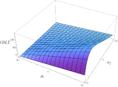
Figure 1: Evolution of GSLT for the model $f(T,T_{G})=-T+\alpha_{1}\sqrt{T^{2}+\alpha_{2}{T_{G}}}$ in terms of coupling parameters $\alpha_{1}$ and $\alpha_{2}$.

Cosmic expansion history is thought to have experienced the decelerated phase and hence transition to accelerating epoch. Thus, power law solutions can play vital role to connect the matter dominated phase with accelerating paradigm. The existence of power law solutions in FRW setting is particularly relevant to intimate all possible cosmic evolutions. The scale factor for power law cosmology is defined as

$$a(t)=a_{0}t^{m},$$

where $m$ is a positive real number. If $0<m<1$, then the required power law solution is decelerating while for $m>1$ it exhibits accelerating behavior. To be more explicit for the above constraint, we set the power law cosmology for accelerated cosmic expansion ($m>1$). For FRW universe, we show the evolution of GSLT in Figure 2. It can be seen that validity of GSLT requires $m>2$ with $\alpha_{1}=14$ and $\alpha_{2}=0.02$.

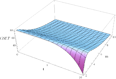
Figure 2: Evolution of GSLT for the model $f(T,T_{G})=-T+\alpha_{1}\sqrt{T^{2}+\alpha_{2}{T_{G}}}$ versus $m$ and $t$ with coupling parameters $\alpha_{1}=14$ and $\alpha_{2}=0.02$.

• $f(T,T_{G})=-T+\beta_{1}\sqrt{T^{2}+\beta_{2}T_{G}}+\alpha_{1}T^{2}+\alpha_{2}T\sqrt{|T_{G}|}$

This model is modified version of previous model and involves higher order correction terms like $T^{2}$ and $T\sqrt{|T_{G}|}$. Here, one can find the derivatives $f$ as

$$\dot{f}_{T} = -1+\beta_{1}T\dot{T}(T^{2}+\beta_{2}T_{G})^{-1/2}+2\alpha_{1}T\dot{T}+\alpha_{2}\dot{T}\sqrt{|T_{G}|},$$

$$\dot{f}_{T} = [\{\beta_{1}(T^{2}+\beta_{2}T_{G})^{-1/2}+2\alpha_{1}\}\dot{T}-\{\beta_{1}T^{2}\dot{T}+\frac{1}{2}\beta_{1}\beta_{2}T\dot{T}_{G}\}(T^{2}+\beta_{2}T_{G})^{-3/2}$$

$$+ \frac{\alpha_{2}}{2}(|T_{G}|)^{-1/2}\dot{T}_{G}],$$

$$\dot{f}_{T_{G}} = [\{-\frac{1}{2}\beta_{1}\beta_{2}T(T^{2}+\beta_{2}T_{G})^{-3/2}+\frac{\alpha_{2}}{2}(|T_{G}|)^{-1/2}\}\dot{T}+\{-\frac{\beta_{1}\beta_{2}^{2}}{4}(T^{2}+\beta_{2}T_{G})^{-3/2}$$

$$- \frac{\alpha_{2}T}{4}(|T_{G}|)^{-3/2}\}\dot{T}_{G}],$$

$$\ddot{f}_{T_{G}} = \{-\frac{\beta_{1}\beta_{2}}{2}(T^{2}+\beta_{2}T_{G})^{-3/2}+\frac{3\beta_{1}\beta_{2}}{2}T^{2}(T^{2}+\beta_{2}T_{G})^{-5/2}\}\dot{T}^{2}+2\{\frac{3}{4}\beta_{1}\beta_{2}^{2}T(T^{2}$$ (35)

$$+ \beta_{2}T_{G})^{-5/2}-\frac{\alpha_{2}}{4}(|T_{G}|)^{-3/2}\}\dot{T}\dot{T}_{G}+\{\frac{3}{8}\beta_{1}\beta_{2}^{3}(T^{2}+\beta_{2}T_{G})^{-5/2}$$

$$+ \frac{3\alpha_{2}T}{8}(|T_{G}|)^{-5/2}\}\ddot{T}_{G}.$$

Using the derivatives (35), we can represent the GSLT as

$$T_{h}\dot{S}_{tot} = \frac{-\dot{H}}{2GH^{4}}(2H^{2}+\dot{H})-\frac{2\pi}{H^{4}}(H^{2}+\dot{H})\left[4H\{(\beta_{1}(T^{2}+\beta_{2}T_{G})^{-1/2}+2\alpha_{1})\dot{T}\right.$$ (36)

$$- \left.(\beta_{1}T^{2}\dot{T}+\frac{1}{2}\beta_{1}\beta_{2}T\dot{T}_{G})(T^{2}+\beta_{2}T_{G})^{-3/2}+\frac{\alpha_{1}}{2}(|T_{G}|)^{-1/2}\dot{T}_{G}\}+4\dot{H}\{-1\right.$$

$$+ \left.\beta_{1}T\dot{T}(T^{2}+\beta_{2}T_{G})^{-1/2}+2\alpha_{1}T\dot{T}+\alpha_{2}\dot{T}\sqrt{|T_{G}|}\}+(8H^{3}-16H\dot{H})\right.$$

$$\times \left.\{(\frac{-\beta_{1}\beta_{2}}{2}T(T^{2}+\beta_{2}T_{G})^{-3/2}+\frac{\alpha_{2}}{2}(|T_{G}|)^{-1/2})\dot{T}+(-\frac{\beta_{1}\beta_{2}^{2}}{4}(T^{2}+\beta_{2}T_{G})^{-3/2})\right.$$

$$- \left.\frac{\alpha_{2}T}{4}(|T_{G}|)^{-3/2})\dot{T}_{G}\}-8H^{2}\{(-\frac{\beta_{1}\beta_{2}}{4}(T^{2}+\beta_{2}T_{G})^{-3/2}+\frac{3\beta_{1}\beta_{2}}{2}T^{2}(T^{2}\right.$$

$$+ \left.\beta_{2}T_{G})^{-5/2})\dot{T}^{2}+(\frac{3}{2}\beta_{1}\beta_{2}^{2}T(T^{2}+\beta_{2}T_{G})^{-5/2}-\frac{\alpha_{2}}{2}(|T_{G}|)^{-3/2})\dot{T}\dot{T}_{G}\right.$$

$$+ \left.(\frac{3}{8}\beta_{1}\beta_{2}^{3}(|T_{G}|)^{-5/2}+\frac{3\alpha_{2}T}{8}(|T_{G}|)^{-5/2})\ddot{T}_{G}\}\right].$$

We first analyze the evolution of GSLT in terms of present day values of cosmic parameters and show the respective behavior in Figure 3. In left plot we present the validity of GSLT in terms of parameters $\beta_{i}$, which can be met only if $\alpha_{i}<0$. Similarly, in right plot we fix $\beta_{i}$ and GSLT is satisfied if $\alpha_{i}<0$. Furthermore, we consider the power law cosmology and present the validity of GSLT in term of $t$ and $m$ as shown in Figure 4.

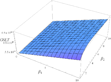
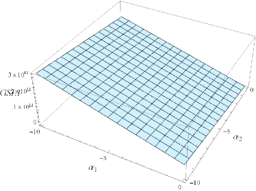
Figure 3: Evolution of GSLT for the model $f(T,T_{G})=-T+\beta_{1}\sqrt{T^{2}+\beta_{2}T_{G}}+\alpha_{1}T^{2}+\alpha_{2}T\sqrt{|T_{G}|}$ versus the parameters $\alpha_{i}(i=1,2)$ and $\beta_{i}(i=1,2)$. The left plot corresponds to parameters $\alpha_{1}=-0.2$ and $\alpha_{2}=-0.1$ and right plot corresponds to $\beta_{1}=0.2$ and $\beta_{2}=2$.

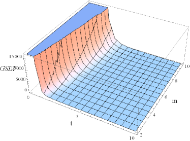
Figure 4: Evolution of GSLT for the model $f(T,T_{G})=-T+\beta_{1}\sqrt{T^{2}+\beta_{2}T_{G}}+\alpha_{1}T^{2}+\alpha_{2}T\sqrt{|T_{G}|}$ versus $m$ and $t$ with $\alpha_{1}=-0.2$, $\alpha_{2}=0.1$, $\beta_{1}=0.2$ and $\beta_{2}=0.1$.

• $f(T,T_{G})=-T+\beta_{1}(T^{2}+\beta_{2}T_{G})+\beta_{3}(T^{2}+\beta_{4}T_{G})^{2}$

Here, $f(T,T_{G})$ model involves fourth order torsion terms and second order contribution from $T_{G}$. For this model, the derivatives of $f$ are obtained as

$$f_{T} = -1+2\beta_{1}T+4\beta_{3}T(T^{2}+\beta_{4}T_{G}),$$

$$\dot{f}_{T} = (2\beta_{1}+12\beta_{3}T^{2}+4\beta_{3}\beta_{4}T_{G})\dot{T}+4\beta_{3}\beta_{4}T\dot{T}_{G},$$

$$\dot{f}_{T_{G}} = 4\beta_{3}\beta_{4}T\dot{T}+2\beta_{3}\beta_{4}^{2}\dot{T}_{G},$$

$$\ddot{f}_{T_{G}} = 4\beta_{3}\beta_{4}\dot{T}^{2}+4\beta_{3}\beta_{4}T\ddot{T}+2\beta_{3}\beta_{4}^{2}\ddot{T}_{G}.$$

Using the above expressions we find constraint for GSLT of the form

$$T_{h}\dot{S}_{tot} = \frac{-\dot{H}}{2GH^{4}}(2H^{2}+\dot{H})-\frac{2\pi}{H^{4}}(H^{2}+\dot{H})\left[4H\{(2\beta_{1}+12\beta_{3}T^{2}+4\beta_{3}\beta_{4}T_{G})\dot{T}\right.$$ (37)

$$+ \left.4\beta_{3}\beta_{4}T\dot{T}_{G}\}+4\dot{H}\{-1+2\beta_{1}T+4\beta_{3}(T^{2}+\beta_{4}T_{G})T\}+(8H^{3}-16H\dot{H})\right.$$

$$\times \left.\{(2\beta_{1}+12\beta_{3}T^{2}+4\beta_{3}\beta_{4}T_{G})\dot{T}+4\beta_{3}\beta_{4}T\dot{T}_{G}\}-8H^{2}\{4\beta_{3}\beta_{4}(\dot{T}^{2}+T\ddot{T})\right.$$

$$+ \left.2\beta_{3}\beta_{4}^{2}\ddot{T}_{G}\}\right].$$

One can see that constraint (37) depends only on the parameters $\beta_{1}$, $\beta_{3}$ and $\beta_{4}$. To specify the values of these parameters we consider recent cosmic parameters (34) and show the evolution of GSLT in left plot of Figure 5. In right plot we consider the power law cosmology and fix $\beta_{i}$ to find variation to find variation of GSLT versus $m$ and $t$.

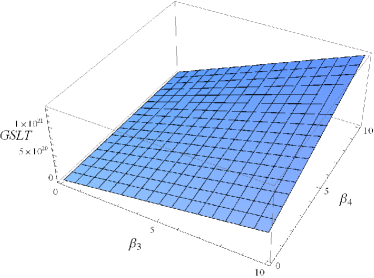
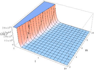
Figure 5: Evolution of GSLT for the model $f(T,T_{G})=-T+\beta_{1}(T^{2}+\beta_{2}T_{G})+\beta_{3}(T^{2}+\beta_{4}T_{G})^{2}$. In left plot we fix the $\beta_{1}=2$ and show the variation of $\beta_{3}$ and $\beta_{4}$. The right plot shows the evolution of GSLT in terms of parameter $m$ and time $t$ with $\beta_{1}=.1$, $\beta_{3}=1$ and $\beta_{4}=2$.

5 Concluding Remarks

In this paper, the thermodynamics properties have been discussed in $f(T,T_{G})$ theory, where $T$ stands for torsion and $T_{G}$ represents the teleparallel equivalent of the Gauss-Bonnet term. We present the equilibrium picture of thermodynamics at the apparent horizon of FRW spacetime. We show that field equations can be cast to the form of FLT $TdS=-dE+dW$. We find that no entropy production term is produced in this work as compared to modified theories involving curvature matter coupling [29]-[31]. The results of this theory coincide with that in Einstein, Gauss-Bonnet, Lovelock and braneworld modified theories [8]-[10].

We also explore the validity of GSLT in the framework of $f(T,T_{G})$ gravity. In this perspective, we consider three generic $f(T,T_{G})$ models namely, $f(T,T_{G})=-T+\alpha_{1}\sqrt{T^{2}+\alpha_{2}{T_{G}}}$, $f(T,T_{G})=-T+\beta_{1}\sqrt{T^{2}+\beta_{2}T_{G}}+\alpha_{1}T^{2}+\alpha_{2}T\sqrt{|T_{G}|}$, and $f(T,T_{G})=-T+\beta_{1}(T^{2}+\beta_{2}T_{G})+\beta_{3}(T^{2}+\beta_{4}T_{G})^{2}$. We set the constraint for GSLT in terms of present day values of Hubble, deceleration, jerk and snap parameters. In Figure 1, we show the evolution of GSLT for model 1 and it is found to be satisfied if $\alpha_{i}>0$. In this discussion we further consider the power law cosmology and found the constraints for accelerated cosmic expansion. Figure 2 shows that GSLT can be met for $m>2$ with $\alpha_{1}=14$ and $\alpha_{2}=0.02$. For second model one requires coupling parameters $\alpha_{i}<0$ with $\beta_{i}>0$. Moreover in case of model 3, we fix $\beta_{1}=2$ and show the variation of $\beta_{3}$ and $\beta_{4}$ in left plot of Figure 5. In right plot the evolution of GSLT for power law cosmology with fixed parameters $\beta_{i}$.

References

• [1] Hawking, S.W.: Commun. Math. Phys. 43(1975)199; Bekenstein, J.D.: Phys. Rev. D 7(1973)2333.
• [2] Bardeen, J.M., Carter, B. and Hawking, S.W.: Commun. Math. Phys. 31(1973)161.
• [3] Jacobson, T.: Phys. Rev. Lett. 75(1995)1260.
• [4] Frolov, A.V. and Kofman, L.: JCAP 05(2003)009.
• [5] Padmanabhan, T.: Class. Quantum Grav. 19(2002)5387.
• [6] Paranjape, A., Sarkar, S. and Padmanabhan, T.:Phys. Rev. D 74(2006)104015; Kothawala, D. and Padmanabhan, T.: Phys. Rev. D 79(2009)104020.
• [7] Cai, R.G. and Kim, S.P.: JHEP 02(2005)050.
• [8] Cai, R.G. and Cao, L.M.: Nucl. Phys. B 785(2007)135.
• [9] Sheykhi, A., Wang, B. and Cai, R.G.: Nucl. Phys. B 779(2007)1.
• [10] Sheykhi, A., Wang, B. and Cai, R.G.: Phys. Rev. D 76(2007)023515.
• [11] Akbar, M. and Cai, R.G.: Phys. Rev. D 75(2007)084003.
• [12] Eling, C., Guedens, R. and Jacobson, T.: Phys. Rev. Lett. 86(2006)121301.
• [13] Cai, R.G. and Cao, L.M.: Phys. Rev. D 75(2007)064008.
• [14] Bamba, K. and Geng, C.Q.: Phys. Lett. B 679(2009)282; JCAP 06(2010)014; ibid. 11(2011)008; Bamba, K., Geng, C.Q. and Tsujikawa, S.: Phys. Lett. B 668(2010)101; Bamba, K., Geng, C.Q., Nojiri, S., and Odinstov, S.D.: Europhys. Lett. 89(2010)50003; Bamba, K., Jamil, M., Momeni, D. and Myrzakulov, R.: Astrophys. Space Sci. 344(2013)259.
• [15] Wu, S.-F., Wang, B., Yang, G.-H. and Zhang, P.-M.: Class. Quantum Grav.25(2008)235018; Sheylhi, A., Teimoori, Z. and Wang, B.: Phys. Lett. B 718(2013)1203.
• [16] Jamil, M., Saridakis, E.N. and Setare, M.R.: JCAP 11(2010)032.
• [17] Wu, S.-F., Wang, B., Yang, G.-H. and Zhang, P.-M.: Class. Quantum Grav. 25(2008)235018.
• [18] Sadjadi, H.M.: Phys. Rev. D 73(2006)063525; ibid. 76(2007)104024; Phys. Lett. B 645(2007)108.
• [19] Karami, K. and Abdolmaleki, A.: JCAP 04(2012)007.
• [20] Sheykhi, A., Wang, B. and Cai, R.G.: Nucl. Phys. B 779(2007)1; Phys. Rev. D 76(2007)023515; Sheykhi, A.: Phys. Rev. D 87(2013)024022.
• [21] Nojiri, S. and Odintsov, S.D.: Int. J. Geom.Meth. Mod. Phys. 4(2007)115; Phys.Rept. 505(2011)59; De Felice, A., Tsujikawa, S.: Living Rev. Rel. 13(2010)03; Bamba, K. Capozziello, S. Nojiri, S. and Odintsov, S.D.: Astrophys. Space Sci. 345(2012)155.
• [22] Bertolami, O., Harko, T., Lobo, F.S.N. and Pa ramos, J.: The Problems of Modern Cosmology (Tomsk State Pedagogical University Press, 2009); Harko, T., Lobo, F.S.N., Nojiri, S. and Odintsov, S.D.: Phys. Rev. D 84(2011)024020; Sharif, M. and Zubair, M.: J. Phys. Soc. Jpn. 81(2012)114005; ibid. 82(2013)014002; ibid. 82(2013)064001; Houndjo, M.J.S.: Int. J. Mod. Phys. D 21(2012)1250003; Alvarenga, F.G. et al.: Phys. Rev. D 87(2013)103526; Odinstov, S.D. and Saez-Gomez, D.: Phys. Lett. B 725(2013)437; Haghani, Z., Harko, T., Lobo, F.S.N., Sepangi, H.R. and Shahidi, S.: Phys. Rev. D 88(2013)044023; Sharif, M., Zubair, M.: Gen. Relativ. Gravit. 46, 1723(2014); Sharif, M., Zubair, M.: Astrophys. Space Sci. 349, 29(2014).
• [23] Moller, C.: Mat. Fys. Skr. Dan. Vid. Selsk. 1(1961)10; Pellegrini, C. and Plebanski, J.: Mat. Fys. Skr. Dan. Vid. Selsk. 2(1963)4.
• [24] Harko, T., Lobo, F.S.N., Otalora, G. and Saridakis, E.N.: Phys. Rev. D 89(2014)124036.
• [25] Zubair, M. and Waheed, S.: Astrophys. Space Sci. 355(2014)361.
• [26] Zubair, M.: Thermodynamic laws in modified gravity with non-minimal torsion matter coupling (Submitted)
• [27] Kofinas, G. and Saridakis, E.N.: Phys. Rev. D 90(2014)084044; Phys. Rev. D 90(2014)084045; Kofinas, G., Leon, G. and Saridakis, E.N.: Class. Quantum Grav. 31(2014)175011.
• [28] Waheed, S. and Zubair, M.: arXiv:1503.07413
• [29] Sharif, M. and Zubair, M.: JCAP 03(2012)028; J. Exp. Theor. Phys. 117(2013)248.
• [30] Sharif, M. and Zubair, M.: Adv. High Energy Phys. 2013(2013)947898.
• [31] Sharif, M. and Zubair, M.: JCAP 11(2013)042.
• [32] Hayward, S.A.: Class. Quantum Grav. 15(1998)3147; Hayward, S.A., Mukohyama, S. and Ashworth, M.: Phys. Lett. A 256(1999)347.
• [33] Izquierdo, G. and Pavon, D.: Phys. Lett. B 633(2006)420.
• [34] Rapetti, D. et al.: Mon. Not. R. Astron. Soc. 375(2007)1510; Riess, A. G. et al.: Astrophys. J. 730(2011)119; N. J. Poplawski: Class. Quantum Grav. 24(2007)3013.