Dynamics of a bond-disordered $S=1$ quantum magnet near $z=1$ criticality

Abstract

Neutron scattering is used to study NiCl_2-2xBr${}_{2x}\cdot$4SC(NH₂)₂, $x=0.06$, a bond-disordered modification of the well-known gapped $S=1$ antiferromagnetic quantum spin system NiCl${}_{2}\cdot$4SC(NH₂)₂. The magnetic excitation spectrum throughout the Brillouin zone is mapped out at $T=60$ mK using high-resolution time-of-flight spectroscopy. It is found that the dispersion of spin excitation is renormalized, as compared to that in the parent compound. The lifetime of excitations near the bottom of the band is substantially decreased. No localized states are found below the gap energy $\Delta\simeq 0.2$ meV. At the same time, localized zero wave vector states are detected above the top of the band. The results are consistent with a more or less continuous random distribution of bond strengths, and a discrete, possibly bimodal, distribution of single-ion anisotropies in the disordered material.

I Introduction

Quantum magnets with disorder and randomness are presently attracting a great deal of attention.Glarum et al. (1991); Fisher (1994); Vojta (2006); Zheludev and Roscilde (2013) They often exhibit behavior that is qualitatively different from that of their disorder-free counterparts. There are actually several ways to introduce randomness in a magnetic material. The effect of site disorder (or site dilution) is rather well understood. Randomly removing spins has particularly severe consequences for gapped quantum paramagnets. Their non-magnetic ground state is destroyed, and magnetic order often emerges at finite temperatures through the formation of correlated clusters around the impurities.Shender and Kivelson (1991); Uchiyama et al. (1999); Uchinokura (2002); Smirnov and Glazkov (2007) In contrast, the effect of random exchange interactions, or bond disorder, is more subtle. In systems with a spin gap the ground state may survive. However, materials close to a magnetic quantum-critical point (QCP) are more drastically affected. Indeed, near QCP even a small variation in the Hamiltonian parameters may lead to the qualitative change of the ground state.Sachdev (2011, 2000, 2008) Recently, VojtaVojta (2013) has numerically investigated the effect of bond disorder on the dynamic properties of a gapped quantum magnet in the vicinity of the $z=1$ QCP. Among the predictions are some intriguing disorder-induced features, such as localized states inside the gap, or the possibility of “weak ordering”. Unfortunately, despite the rapid increase in the number of organometallic quantum magnets,Landee and Turnbull (2013) and the ease of achieving bond disorder via chemical substitution on nonmagnetic sites involved in superexchange,Yankova et al. (2012) there is presently a shortage of suitable model compounds to test the predictions of Ref. Vojta, 2013. Most of the known gapped quantum magnets (e. g. TlCuCl₃,Oosawa and Tanaka (2002) IPA-CuCl₃,Náfrádi et al. (2013) PHCC,Hüvonen et al. (2012, 2012, 2013); Glazkov et al. (2014) Sul-Cu₂Cl₄,Wulf et al. (2011) Cu(Qnx)Cl₂Keith et al. (2011); Povarov et al. (2014)) exhibit a “blue shift” of magnons in the presence of bond disorder. Thus, chemical modification increases the spin gap and pushes these systems away from the $z=1$ QCP.

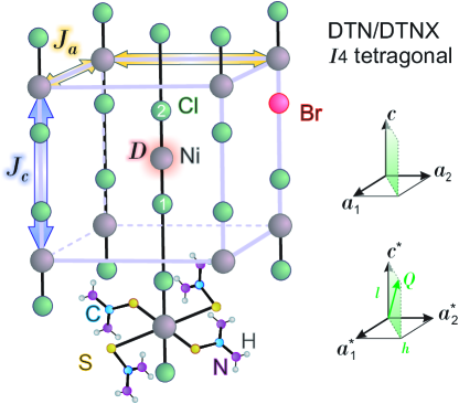
Figure 1: (Color online) A sketch of the NiCl_2-2xBr${}_{2x}\cdot$4SC(NH₂)₂ structure. The surrounding thiourea units are shown only for one of the Ni²⁺ ions. The main magnetic interactions (see Hamiltonian (1)) for $S=1$ nickel ions are labeled. Two non-equivalent chlorine positions are marked as 1 and 2. The scattering plane for the present neutron experiment is shown on the right, in both real (top) and reciprocal (bottom) space representations.

One known exception is the extensively studied $S=1$ gapped quantum magnet dichlorotetrakis-thiourea nickel NiCl${}_{2}\cdot$4SC(NH₂)₂ (commonly abbreviated as DTN).Paduan-Filho et al. (1981); Zapf et al. (2006); Zvyagin et al. (2007); Yin et al. (2008); Mukhopadhyay et al. (2012); Tsyrulin et al. (2013); Wulf et al. (2015) In contrast to integer-spin Heisenberg magnets such as CsNiCl₃,Kenzelmann et al. (2001); Zaliznyak et al. (2001) the gap in DTN is due to huge planar single-ion anisotropy. The three-dimensional interactions in DTN are also strong enough to make the Haldane gap physics irrelevant.Haldane (1983); Sakai and Takahashi (1990) Bond disorder is introduced into DTN by a random Br substitution on the Cl site. This actually produces a “red shift” (decrease) of the spin gap.Yu et al. (2012); Wulf et al. (2013) In this respect, Br-substituted DTN, NiCl_2-2xBr${}_{2x}\cdot$4SC(NH₂)₂ (below abbreviated as DTNX), appears to be the most promising candidate for an experimental realization of the physics discussed in Ref. Vojta, 2013.

The present work is a study of spin dynamics in DTNX with $x=6$% Br substitution. High-resolution inelastic neutron scattering experiments provide a detailed picture of magnetic excitations throughout the Brillouin zone. The measured spectra exhibit certain key differences compared to the parent material: an increase of the bandwidth, a reduction of excitation lifetimes, and new localized states at high energies. We discuss the relation between these experimental results and the numerical predictions of Ref. Vojta, 2013. In addition, we touch on the relevance of our findings to the previous thermodynamic studies of DTNX in applied magnetic fields.Yu et al. (2012); Wulf et al. (2013)

The paper is organized as follows: In Sec. II we review the structure and magnetic properties of our target material, and describe the experimental setup and techniques; a brief overview of the collected data is given in Sec. III, followed by detailed analysis and discussion in Sec. IV; Sec. V summarizes our conclusions and outlines the future research directions; some more technical issues are laid out in the appendixes.

II Material and experimental details

II.1 The parent and disordered compounds

Disorder-free DTN NiCl${}_{2}\cdot$4SC(NH₂)₂ is an organometallic magnet belonging to a highly symmetric $I4$ tetragonal space group.Lopez-Castro and Truter (1963) Magnetic $S=1$ Ni²⁺ ions occupy the positions in the body-centered tetragonal lattice (see Fig. 1) with $a=9.558$ Å and $c=8.981$ Å. Due to this body-centered arrangement, the magnetic system can be seen as a combination of two interpenetrating tetragonal lattices that are totally decoupled at the mean-field level. Within each of these subsystems the magnetic properties are captured by the following Hamiltonian:

$${{\mathcal{H}}}=\sum\limits_{\left\langle i,j\right\rangle,n}D(S^{z}_{in})^{2}+J_{c}\textbf{S}_{in}\textbf{S}_{i(n+1)}+J_{a}\textbf{S}_{in}\textbf{S}_{jn},$$ (1)

where $\left\langle i,j\right\rangle$ is the summation over the nearest neighbors in the tetragonal $(a,a)$ plane, and index $n$ refers to the summation along the $c$ axis. The magnetic properties are dominated by the strong single-ion anisotropy of easy-plane type $D\simeq 0.78$ meV. The next term in the magnetic hierarchy is the nearest-neighbor Heisenberg exchange interaction $J_{c}\simeq 0.141$ meV within the chains running along the high-symmetry axis. The least important interaction is the interchain coupling $J_{a}\simeq 0.014$ meV, which is an order of magnitude weaker than $J_{c}$.Zapf et al. (2006) As a result of the huge anisotropy, the ground state of DTN is a quantum-disordered XY paramagnet with a spin-singlet nonmagnetic ground state and a spin gap $\Delta\simeq 0.3$ meV.

It has been previously demonstrated that Br substitution has a very slight effect on the lattice parameters and does not affect the symmetry.Yu et al. (2012) The bromine ions are site selective: They occupy Cl-1 positions in the lattice as shown in Fig. 1. Chemical substitution decreases the critical field $H_{c1}$ of magnetic ordering in DTNX, indicating a reduced spin gap.Yu et al. (2012); Wulf et al. (2013) This gap reduction is significant: Already at $x=13$% bromine concentration $\Delta\simeq 0.1$ meV is almost three times smaller than in the parent compound.

II.2 Quantities measured

Magnetic inelastic neutron scattering almost directly probes the dynamic spin structure factor:

$$\mathcal{S}^{\alpha\beta}(\mathbf{Q},\omega)=\int e^{-i[(\mathbf{Q}\cdot\mathbf{r})-\omega t]}\left\langle S^{\alpha}(0,0)S^{\beta}(\mathbf{r},t)\right\rangle\dfrac{d^{3}\mathbf{r}dt}{2\pi}.$$ (2)

The actual neutron intensity measured in experiments is proportional to the differential cross section, and for unpolarized neutrons is given by: Squires (2012)

$$I(\mathbf{Q},\omega)\propto\frac{d^{2}\sigma}{dEd\Omega}\propto F^{2}(Q)\sum_{\alpha}\left(1-\frac{Q_{\alpha}^{2}}{Q^{2}}\right)\mathcal{S}^{\alpha\alpha}(\mathbf{Q},\omega).$$ (3)

Here $\mathbf{Q}$ and $\hbar\omega$ the momentum and energy transfers, respectively. $F^{2}(Q)$ is the magnetic form factor for Ni²⁺, known from numerical calculations.Prince (2004) No absolute normalization of the data was performed in this study.

II.3 Experimental setup

In the present work we used large (mass $\sim 1$ g) fully deuterated single crystals of DTNX with 6% Br substitution. They were grown from the solution by the same method as in previous works.Paduan-Filho et al. (2004); Zapf et al. (2006); Yu et al. (2012); Wulf et al. (2013) The measurements were carried out on the high resolution cold neutron time-of-flight (TOF) spectrometer IN5 at Institut Laue–Langevin.Ollivier and Mutka (2011) Sample environment was a ³He-⁴He dilution cryostat. All data were collected on two co-aligned single crystals at $T=60$ mK, which is much lower than all the relevant energy scales of DTN. The principal experimental scattering plane was $(1,-1,0)$, providing access to scattering vectors of type $(h,h,l)$ (see Fig. 1). Two data sets were collected, using incident neutron energies $E_{\text{i}}=2.26$ and $1.17$ meV, respectively. A Gaussian fit to the elastic incoherent scattering provided an estimate of the energy resolution: $\sqrt{8\ln 2}\sigma\simeq 38~{}\mu$eV and $16~{}\mu$eV full width at half height, respectively. In the high-resolution setup, incoherent elastic scattering has virtually no effect on the data collected above $\hbar\omega=25~{}\mu$eV energy transfer. For each incident energy, the sample was rotated step-wise through the data collection, to fully cover the first Brillouin zone.

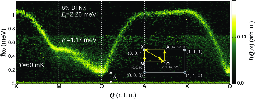
Figure 2: (Color online) False color plot of the neutron scattering intensity measured in 6% DTNX at $T=60$ mK. The data are presented as a multi-panel cut along the trajectory shown in the inset. The data collected with $E_{\text{i}}=2.26$ and 1.17 meV incident energy are combined in each panel. The integration range in $\mathbf{Q}$ transverse to the cut directions is $\pm 0.02$ reciprocal lattice units.

III Data overview

The bulk of the neutron TOF data collected in 6% DTNX at $T=60$ mK is visualized in Fig. 2. These are a series of false color plots of the measured inelastic intensity, presented as two-dimensional momentum-energy cuts along high-symmetry directions. The data below and above $0.7$ meV energy transfer were taken with neutron incident energies $E_{\text{i}}=1.17$ meV and $E_{\text{i}}=2.26$ meV, respectively. We stress that the data are plotted “as is”, without any background subtraction.

The measured spectrum of 6% DTNX is qualitatively similar to that of disorder-free DTN.Zapf et al. (2006) It is dominated by a well-defined magnon mode with a dispersion minimum at the antiferromagnetic zone center $\text{{O}}=(1/2,1/2,1/2)$. Two saddle points are located at $\text{{M}}=(0,0,1/2)$ and $\text{{A}}=(1/2,1/2,0)$, correspondingly. The highest energy of the single-magnon excitation is found at $\text{{X}}=(0,0,0)$. The main difference with the parent material is a much reduced spin gap $\Delta\simeq 0.2$ meV, compared to $\Delta\simeq 0.3$ meV in DTN.

At lower energies, the excitations in DTNX appear less sharp than at high energy transfers. Notably, there are no additional excited states below the gap energy at the O point or any other region of the Brillouin zone down to $25$ $\mu$eV. Finally, we note a subtle drop of intensity around $0.4$ meV. The latter is found in data sets with both neutron incident energies, and hence is unlikely to be of instrumental origin. Although it resembles an avoided crossing in the false-color plot shown, it is actually always observed at the same energy transfer, irrespective of wave vector. Its origin remains unclear.

IV Analysis and discussion

IV.1 Dispersive excitations

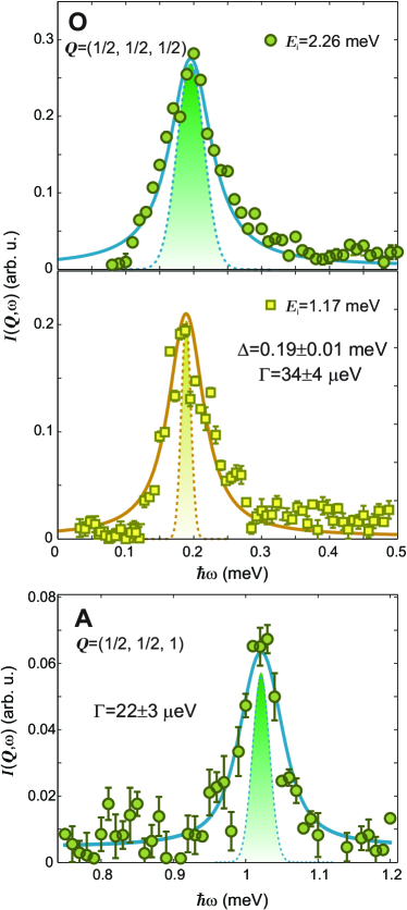
Figure 3: (Color online) Constant-$\mathbf{Q}$ cuts at the center (O) and at the boundary (A) of antiferromagnetic Brillouin zone of 6% DTNX. Squares and circles correspond to $E_{\text{i}}=1.17$ meV and $E_{\text{i}}=2.26$ meV, respectively. Voigt fits (4) are shown by solid lines. The shaded areas represent the experimental energy resolution.

		DTN		6% DTNX
		Zapf et al. (2006)Zapf et al. (2006)		Present study Eq. (1) only		Present study Eq. (1)$+J_{d}$		Present study Eq. (1)$+J_{c2}$		Present study Eq. (1)$+J_{d}+J_{c2}$
$D$		$0.780(3)$ meV		$0.792(3)$ meV		$0.812(2)$ meV		$0.805(2)$ meV		$0.807(2)$ meV
$J_{c}$		$0.141(3)$ meV		$0.155(1)$ meV		$0.158(1)$ meV		$0.149(1)$ meV		$0.150(1)$ meV
$J_{a}$		$0.014(1)$ meV		$0.0158(3)$ meV		$0.0161(2)$ meV		$0.0155(2)$ meV		$0.0157(2)$ meV
$J_{d}$		-		-		$0.0059(5)$ meV		-		$0.0060(4)$ meV
$J_{c2}$		-		-		-		$-0.0095(7)$ meV		$-0.0096(7)$ meV
$D/J_{c}$		$5.5(1)$		$5.11(3)$		$5.14(3)$		$5.40(3)$		$5.38(3)$
$J_{a}/J_{c}$		$0.098(7)$		$0.102(2)$		$0.102(2)$		$0.104(2)$		$0.105(2)$

Table 1: Results of fitting the RPA dispersion relation (5) to the measured excitation energies in 6% DTNX. Additional perturbations to the basic Hamiltonian (1) are considered (see Appendix A for more details). The results of an analogous analysis for disorder-free DTN from Ref. Zapf et al., 2006 are also shown.

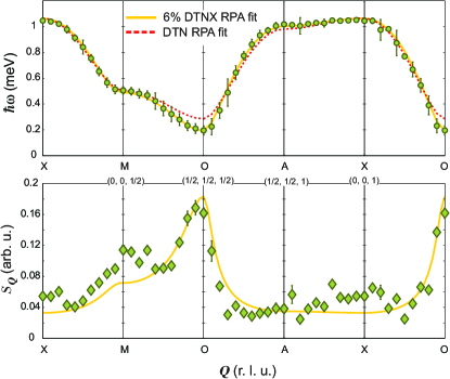
Figure 4: (Color online) Top panel: Magnon dispersion relation measured in 6% DTNX, as deduced from Voigt fits to individual constant-$\mathbf{Q}$ cuts of $E_{\text{i}}=2.26$ meV dataset. The solid line is a fit to the RPA prediction of Eq. (5) with the parameters summarized in the last column of Table 1. The dashed line is the reference magnon dispersion in disorder-free DTN following Ref. Zapf et al., 2006. Bottom panel: Integrated intensity corrected for the magnetic form factor and polarization factor, $\mathcal{S}_{\mathbf{Q}}$, as determined in fits to the same individual cuts. The solid line is the RPA result, which is simply the inverse of $\hbar\omega_{\mathbf{Q}}$.

Since we lack a suitable microscopic model to globally describe the spectrum in a quantum magnet with disorder, we chose a more empirical approach to data analysis. We quantitatively analyze the $E_{\text{i}}=2.26$ meV dataset, covering the full magnetic excitation band. The measured data were broken up into a series of individual constant-$\mathbf{Q}$ cuts. In each such cut, the scattering is a well-defined peak that we approximated by a Voigt profile:

$$I(\mathbf{Q},\omega)=\mathcal{S}_{\mathbf{Q}}F^{2}(Q)\left(2-\frac{Q_{\bot}^{2}}{Q^{2}}\right)V(\hbar\omega-\hbar\omega_{\mathbf{Q}},\sigma,\Gamma_{\mathbf{Q}}).$$ (4)

The Gaussian width $\sigma$ represents experimental energy resolution (the values quoted above, with the energy transfer correction includedLowde (1960); Lechner (1985)). For each cut, the parameters of this model are as follows. $\hbar\omega_{\mathbf{Q}}$ is the position of the peak that we associate with the single-magnon energy. The Lorentian width $\Gamma_{\mathbf{Q}}$ of the Voigt function represents the intrinsic magnon line width and, potentially, wave vector resolution (“focusing”) effects. $\mathcal{S}_{\mathbf{Q}}$ is the peak’s integrated intensity. Due to the planar nature of the ground state, we assumed that the observed magnon corresponds to transverse spin fluctuations $\mathcal{S}^{xx}(\mathbf{Q},\omega)=\mathcal{S}^{yy}(\mathbf{Q},\omega)$. The polarization factors in the expression above are chosen accordingly, with $Q_{\bot}$ being the momentum transfer in the $(a,a)$ plane. Examples of fits to individual cuts can be found in Fig. 3.

The thus obtained magnon dispersion relation is plotted in symbols in the upper panel of Fig. 4. These data were further analyzed within the random-phase approximation (RPA),Jensen and Mackintosh (1991) treating the Heisenberg exchange as a perturbation to decoupled $S=1$ single ions. The RPA dispersion relation is:

$$\hbar\omega_{\mathbf{Q}}=\sqrt{D^{2}+4D\gamma(\mathbf{Q})}.$$ (5)

Here $\gamma(\mathbf{Q})=\sum\limits_{\mathbf{r}}J_{\mathbf{r}}\cos(\mathbf{Qr})$ is essentially the Fourier transform Heisenberg exchange interactions in the system. For our fit, we consider not only the parameters $D$, $J_{c}$ and $J_{a}$, but also two possible perturbations to the Hamiltonian (1): diagonal exchange between the tetragonal sublattices $J_{d}$ and the next-nearest neighbor exchange along the $c$ direction $J_{c2}$. The reasons to introduce these perturbations are discussed in Appendix A. Fitting the RPA dispersion relation to the data in Fig. 4 (top panel) yields the parameter values summarized in Table 1. The fit itself is represented by the solid line. For a direct comparison, we also quote Hamiltonian parameters for disorder-free DTN from the previous studiesZapf et al. (2006) and plot the corresponding dispersion relation in a dashed line.

As the analysis shows, the gap softening in DTNX is primarily due to the increase of the bandwidth. Even as the anisotropy becomes stronger with the Br substitution, the ratio $D/J_{c}$ actually decreases from $5.5$ in pure DTN to $5.1-5.4$ in 6% DTNX, depending on the terms included in the model Hamiltonian. The ratio $J_{a}/J_{c}$ is still around $0.1$ within the uncertainty limit. The RPA dispersion (5) can be modified to account for quantum renormalization of the bare Hamiltonian parameters. This correction, described in Appendix B, changes the $D/J_{c}$ ratio to $4.7$ in the parent material.Zapf et al. (2006); Zhang et al. (2013) In 6% DTNX, as found from the present experiment, it will be between $4.06$ and $4.36$. The ratio $J_{a}/J_{c}\simeq 0.1$ is unchanged. Thus the reduced $D/J_{c}$ ratio is the key ingredient of the excitations “red shift” in DTNX.

The intensities $\mathcal{S}_{\mathbf{Q}}$ obtained in fits to individual cuts are plotted in symbols in the lower panel of Fig. 4. In the RPA, $\mathcal{S}_{\mathbf{Q}}$ is simply proportional to $1/\hbar\omega_{\mathbf{Q}}$. As shown by the solid line, this expectation is in a reasonable agreement with the data. The remaining discrepancies might be attributed to the possible contribution of longitudinal fluctuations, not included in our approach.

IV.2 Approaching criticality

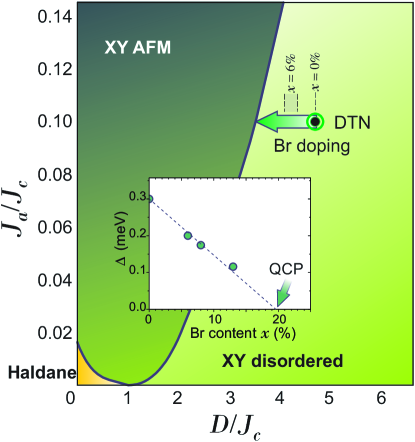
Figure 5: (Color online) Ground states of Hamiltonian (1), based upon the results of Refs. Wierschem and Sengupta, 2014a, b. The arrow indicates the approximate trajectory of DTNX upon Br substitution. The inset shows the energy gap in DTNX as a function of bromine content. Data points are the result of the present and previous studies.Zapf et al. (2006); Yu et al. (2012); Wulf et al. (2013) The dashed line is a guide for the eye.

Due to a random distribution of Br substitutes in the sample, the parameters of the microscopic Hamiltonian, including exchange constants and anisotropy, will themselves vary from one unit cell to the next in a random manner. This said, it stands to reason that the values obtained from analyzing magnon dispersion curves correspond to the average values of these parameters. The main mechanism leading to a decrease of the spin gap and driving DTNX closer to the QCP is a then a steadily decreasing $D/J_{c}$ ratio.

Fortunately, the phase diagram of Hamiltonian (1) is well known numerically,Sakai and Takahashi (1990); Wierschem and Sengupta (2014a, b) and shown in Fig. 5. For small anisotropy and almost isolated chains it includes a gapped topological Haldane phase. Sufficiently strong interchain interactions restore XY-like long range magnetic order. However, the system is again in a gapped non-magnetic “single ion” state for large anisotropy. The values of Hamiltonian parameters determined for the parent DTN compound,Zapf et al. (2006) allow us to place it in the latter region of the phase diagram (see Fig. 5). As mentioned above, Br substitution does not change the $J_{a}/J_{c}$ ratio significantly. Instead, by decreasing $D/J_{c}$, the system is driven left on the phase diagram, towards the line of long-range XY ordering. The inset of Fig. 5 show the energy gap $\Delta$ in DTNX as a function of Br content, as deduced from the current and previous studies.Zapf et al. (2006); Yu et al. (2012); Wulf et al. (2013) The decrease is roughly linear, and the gap may be expected to close around 20% Br content. At present it is not clear whether DTNX samples with such high Br concentrations are stable.

IV.3 Magnon lifetimes

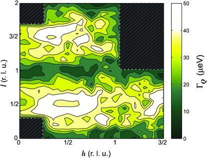
Figure 6: (Color online) False color map of measured intrinsic Lorentian magnon linewidth $\Gamma_{\mathbf{Q}}$ as found from Voigt fits to individual constant-$\mathbf{Q}$ cuts ($E_{\text{i}}=2.26$ meV dataset). Regions of reciprocal space with no data are shown hatched.

Beyond a simple change of average Hamiltonian parameters, several key features of the spectrum are to be attributed to disorder, i.e., to a microscopic random variation of these parameters in the sample. As shown in Fig. 3, the excitations at the antiferromagnetic zone center O have a significant energy width beyond the resolution of the instrument. This is further emphasized by comparing data obtained with different neutron incident energy. For $E_{\text{i}}=1.17$ meV the energy resolution is much sharper than for $E_{\text{i}}=2.26$ meV, but the obtained broad peak at $\mathbf{Q}=(1/2,1/2,1/2)$ is similar in both cases, with effective Lorentian linewidth $\Gamma=34\pm 4$ $\mu$eV. Although at high energies the excitations are sharper, their linewidth is still pronounced. Fitted linewidth at, for instance, point A is $\Gamma=22\pm 3$ meV. As the resolution function of a time-of-flight spectrometer sharpens with the increase in energy transfer,Lowde (1960); Lechner (1985) the linewidth $\Gamma$ still exceeds the estimated instrument resolution $\sigma$ at $\hbar\omega\simeq 1$ meV almost twice.

Wavevector resolution effects alone can not account for the observed increase of linewidth. A conservative estimate of $\mathbf{Q}$-resolution contribution to the peak width in energy cuts can be done as $\sigma_{\mathbf{Q}}\lesssim|\hbar\omega_{\mathbf{Q}+\delta\mathbf{Q}}-\hbar\omega_{\mathbf{Q}}|$. In our case, for the antiferromagnetic zone center this gives only $\sigma_{\mathbf{Q}}\simeq 5$ $\mu$eV, which is much less than the observed broadening.

The contour map of measured intrinsic line width $\Gamma_{\mathbf{Q}}$ is shown in Fig. 6. One can see that $\Gamma_{\mathbf{Q}}$ varies significantly along the tetragonal axis, but has a less pronounced variation in a transverse direction. The broadest excitations are found around the antiferromagnetic zone center where the dispersion is a minimum. This is in a strong contrast with the picture of excitation broadening previously observed in another bond-disordered gapped antiferromagnet PHCX.Hüvonen et al. (2012) In the latter case, magnon damping is due to scattering on isolated (discrete) impurities. As a result, it roughly scales with the single-magnon density of states, and is a maximum at the band top. In DTNX we find exactly the opposite. As will be argued below, the observed behavior of $\Gamma_{\mathbf{Q}}$ is consistent with a smooth continuous distribution of Heisenberg exchange strengths in the material.

IV.4 Localized states

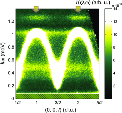
Figure 7: (Color online) High contrast false color map of $I(\mathbf{Q},\omega)$ for $\mathbf{Q}$ along $\mathbf{c}^{\ast}$ (here $E_{\text{i}}=2.26$ meV). The integration range in transverse direction is the entire Brillouin zone. Note the dispersionless (local) excitations just above the top of the magnon band denoted by arrows.

Figure 7 shows a high-contrast false color plot of $I(\mathbf{Q},\omega)$ integrated over the whole Brillouin zone and projected onto a $\mathbf{c}^{\ast}$ direction. Note that here we use a linear intensity scale, compared to the logarithmic scale used above in Fig. 2. In Fig. 7, the magnon band looks completely “overexposed”. There are clearly no additional states visible inside the gap. However, additional states are found just above the top of the band at $\hbar\omega\simeq 1.25$ meV. These are local excitations, as they show no dispersion.

Given the low intensity of the feature in 6% DTNX, how reliable is this observation? An important argument here is that the feature at $1.25$ meV has an intensity distribution, perfectly matching the sample’s reciprocal lattice. The intensity is cosine modulated along $[0~{}0~{}1]$ and constant along $[1~{}1~{}0]$. This is nontypical for the spurious features usually having no $\mathbf{Q}$-structure.Pintschovius et al. (2014) As the numerical calculations show, localized feature of this kind can actually be expected in a bond-disordered systemVojta (2013); Utesov et al. (2014) (this will be discussed in more details below). Indirect evidence of high-energy states in DTNX also comes from the experimentally observed pre-saturation “pseudoplateau” in magnetization.Yu et al. (2012) The width of the plateau $\Delta H\simeq 1.5$ T and the observed energy separation between the band top and the localized state $\hbar\Delta\omega\simeq 0.2$ meV are in a rough agreement. As these states are located at the regions of reciprocal space, equivalent to $Q=0$ momentum transfer, they should also be observable by such techniques as electron spin resonance and THz spectroscopy. A very recent THz spectroscopy experiment does show the presence of an additional feature at approximately the same energy in DTNX and its absence in the parent material.

IV.5 Disorder analysis

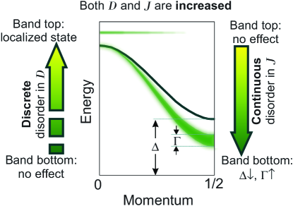
Figure 8: (Color online) A cartoon highlighting the main effects of various kinds of disorder on the spin excitation spectrum. The solid line is the magnon dispersion in the absence of disorder. The blurred curve is the spectrum of the disordered system.

To understand the emergence of local excitations and other features of the observed spectrum, we can establish a crude qualitative “mapping” between the Hamiltonians of DTN (1) and that of the dimer modeled studied in Ref. Vojta, 2013. The latter has two parameters: the intradimer exchange constant $\mathcal{J}$ and the interdimer coupling $\mathcal{K}$. The dimer strength $\mathcal{J}$ primarily determines the gap and interdimer exchange $\mathcal{K}$ determines the bandwidth. The increase of the former drives the system away, and of the latter — closer to QCP. In this sense, our $S=1$ individual magnetic sites with single-ion anisotropy can be seen as spin-gap objects analogous to the $S=1/2$ dimers. The parameter $\mathcal{J}$ is then naturally mapped to the single-ion anisotropy $D$ and the critical coupling $\mathcal{K}$ corresponds to the Heisenberg exchange $J$. Similar mapping between dimerized and single-ion anisotropy systems has also been used in a recent theoretical study of Utesov et al.Utesov et al. (2014)

The numerical study Ref. Vojta, 2013 predicts the presence of in-gap states in two cases of discrete disorder distribution: a small fraction of isolated sites having $\mathcal{J}<\left\langle\mathcal{J}\right\rangle$ (in our correspondence with DTN $D<\left\langle D\right\rangle$) or a small fraction of sites with $\mathcal{K}>\left\langle\mathcal{K}\right\rangle$ (in our case $J>\left\langle J\right\rangle$). Our analysis of the magnon spectrum in DTNX shows that anisotropy $D$ is effectively increased by Br substitution, so the former scenario is clearly not applicable. Thus, not having any in-gap bound states in DTNX may indicate that the disorder of the exchange constant $J$ is either weak or non-discrete. At the same time, as captured by the simulations of Ref. Vojta, 2013 (Fig. 5 therein), a small number of sites with a singular large value of $\mathcal{J}>\left\langle\mathcal{J}\right\rangle$ (i. e. $D>\left\langle D\right\rangle$) produces a localized state near the top of the magnon band. This is totally in line with our observation of high-energy local excitations in DTNX. The underlying assumption is that the anisotropy distribution is discrete, with just a few Ni²⁺ ions having a substantially increased $D$-term. The simulations also predict a broadening of the main magnon branch, in the case of a continuous broad distributions of either $\mathcal{K}$ and $\mathcal{J}$. The former broadens the magnons evenly in the entire Brillouin zone (Ref. Vojta, 2013 Supplementary Material, Fig. S4), while the latter mostly affects magnons at the bottom of the band (Fig. S5). Comparing it to our observations, we may again guess that the exchange constants in DTNX show a rather broad continuous distribution.

Certainly, the above discussion is based on a rather tenuous analogy between two very different Hamiltonians. However, if we accept this qualitative correspondence, the following picture emerges. The average values of both $\langle D\rangle$ and $\langle J\rangle$ are increased with the Br substitution, modifying the magnon dispersion relation accordingly. The anisotropy is decreased on only a few sites, probably in direct proximity of the Br substitutes. The exchange constants, however, have a broad statistical distribution around the average value. Schematically, this scenario is borne out in Fig. 8. A broad distribution of exchange constants in DTNX is not unexpected. It results from each Br substitute affecting a large number of bonds. Each such size-mismatched Br defect creates a strain field in the crystal, which, in turn, affects bond angles and thereby superexchange interactions. The strain field falls off as $\sim r^{-3}$ (Ref. Indenbom and Lothe, 1992), and in a soft material like DTNX is expected to be rather long-range.

V Conclusions

In summary, Br substitution has a profound effect on the spin dynamics of DTN, even at rather low concentrations. On the one hand, both anisotropy and exchange interactions are, on the average, increased. The ratio $D/J_{c}$ actually decreases, reducing the spin gap and driving the system closer to the QCP. Simultaneously, new features emerge due to disorder. Magnon lifetimes are shortened, predominantly at the bottom of the band. Somewhat counter-intuitively, localized states appear not inside the spin gap, but just above the top of the magnon band. This behavior can be explained by a hand-waving analogy with disorder in the Heisenberg-dimer model.Vojta (2013) We hope that our experiments will stimulate a study of randomness in the anisotropic single-ion Hamiltonian appropriate for DTN.

Appendix A Additional interactions

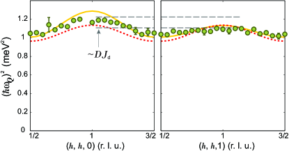
Figure 9: (Color online) Symbols: squared dispersion $(\hbar\omega_{\mathbf{Q}})^{2}$ along the $(h,h,0)$ and $(h,h,1)$ directions ($E_{\text{i}}=2.26$ meV). The dashed line is the dispersion model for pure DTN used by Zapf et al.Zapf et al. (2006). The solid line is best fit with $J_{d}$ perturbation included, as in the last column of Table 1.

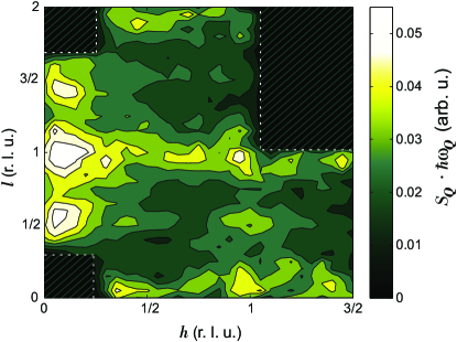
Figure 10: (Color online) Contour map of weighted peak intensity $\mathcal{S}_{\mathbf{Q}}\cdot\hbar\omega_{\mathbf{Q}}$ in the $(h,h,l)$ plane ($E_{\text{i}}=2.26$ meV). Note the half-period modulation along $\mathbf{c}^{\ast}$, i. e. the peaks at both integer and half-integer values of $l$.

Here we describe some features in our inelastic data that point to the presence of additional magnetic interactions, not included in the Hamiltonian (1). The first additional interaction is the so-called “diagonal” Heisenberg exchange between the two tetragonal sublattices. The presence of this exchange $J_{d}$ was already noted in the ESR experiment by Zvyagin et al.Zvyagin et al. (2008) and confirmed in neutron scattering investigation by Tsirulin et al.Tsyrulin et al. (2013) The introduction of $J_{d}$ leads to additional double-period modulation of the dispersion relation. This new periodicity can be indeed spotted in the data. Figure 9 shows a comparison of dispersion curves (actually, dispersion squared) measured along the $(h,h,0)$ and $(h,h,1)$ directions (symbols). The difference between the otherwise equivalent reciprocal-space directions is naturally explained by a non-zero $J_{d}$, as shown by the solid line which corresponds to the best-fit value of $J_{d}$. For comparison, the dashed line is the proposed DTN dispersion from Ref. Zapf et al., 2006, where $J_{d}$ is not included.

The second additional term that we consider is the next-nearest neighbor exchange coupling $J_{c2}$ along the chain direction. The evidence for this term comes from the very specific pattern found in the intensity distribution. The product $\mathcal{S}_{\mathbf{Q}}\cdot\hbar\omega_{\mathbf{Q}}$ shown in Fig. 10 exhibits a half-period modulation along the $\mathbf{c}^{\ast}$ direction. This implies the presence of additional interaction with the translation vector $\mathbf{r}=2\mathbf{c}$. Additionally, $J_{2c}$ manifests itself in a slight “blunting” of the $\cos$-like dispersion along the $c$ axis, near the top of the band. That, too, is consistent with our data. Note that next-nearest-neighbor interactions along the $c$ axis could not be detected in the high-field experiment of Ref. Tsyrulin et al., 2013, as their scattering plane was orthogonal to $\mathbf{c}$. Analyzing the measured dispersion in DTNX, we find $J_{c2}$ to be ferromagnetic, and therefore nonfrustrating. Both $J_{d}$ and $J_{c2}$ corrections are relatively small, and don’t qualitatively affect the general picture for DTN.

Appendix B Self-consistent corrections to the RPA

DTN

6% DTNX

Zapf et al. (2006)Zapf et al. (2006)

Tsirulin et al. (2013)Tsyrulin et al. (2013)

Present study Eq. (1) only

Present study Eq. (1)$+J_{d}$

Present study Eq. (1)$+J_{c2}$

Present study Eq. (1)$+J_{d}+J_{c2}$

$s^{2}$

$0.943$

$-$

$0.921$

$0.923$

$0.926$

$0.924$

$D$

$0.700(3)$ meV

$0.767$ meV

$0.682(3)$ meV

$0.702(2)$ meV

$0.702(2)$ meV

$0.701(3)$ meV

$J_{c}$

$0.150(3)$ meV

$0.177$ meV

$0.168(1)$ meV

$0.171(1)$ meV

$0.161(1)$ meV

$0.162(1)$ meV

$J_{a}$

$0.015(1)$ meV

$0.0134(3)$ meV

$0.0172(5)$ meV

$0.0174(2)$ meV

$0.0167(2)$ meV

$0.0170(5)$ meV

$J_{d}$

-

$0.0069(9)$ meV

-

$0.0064(5)$ meV

-

$0.0065(4)$ meV

$J_{c2}$

-

-

-

-

$-0.0103(7)$ meV

$-0.0104(7)$ meV

$D/J_{c}$

$4.7(1)$

$4.34$

$4.06(3)$

$4.10(3)$

$4.36(3)$

$4.33(3)$

$J_{a}/J_{c}$

$0.098(7)$

$0.076(2)$

$0.102(2)$

$0.102(2)$

$0.104(2)$

$0.105(2)$

Table 2: Results of fitting Eqs. (6-8) to our 6% DTNX dispersion data and to those for the parent compound (Ref. Zapf et al., 2006). For the parent compound, parameters deduced from the spin-wave dispersion measured in the saturated phase, are also listed. Tsyrulin et al. (2013)

		DTN		6% DTNX
		Sizanov and Syromyatnikov (2011)Sizanov and Syromyatnikov (2011)		Present study Eq. (1) only		Present study Eq. (1)$+J_{d}$		Present study Eq. (1)$+J_{c2}$		Present study Eq. (1)$+J_{d}+J_{c2}$
$D$		$0.666$ meV		$0.661(1)$ meV		$0.661(1)$ meV		$0.672(2)$ meV		$0.672(2)$ meV
$J_{c}$		$0.160$ meV		$0.176(1)$ meV		$0.177(1)$ meV		$0.169(1)$ meV		$170(2)$ meV
$J_{a}$		$0.0172$ meV		$0.0190(3)$ meV		$0.0192(2)$ meV		$0.0190(3)$ meV		$0.0193(2)$ meV
$J_{d}$		$0.0086$ meV		-		$0.0075(6)$ meV		-		$0.0075(5)$ meV
$J_{c2}$		-		-		-		$-0.007(1)$ meV		$-0.007(1)$ meV
$D/J_{c}$		$4.16$		$3.75(3)$		$3.73(3)$		$3.96(4)$		$3.95(6)$
$J_{a}/J_{c}$		$0.108$		$0.108(2)$		$0.109(2)$		$0.112(2)$		$0.113(3)$

Table 3: Results of fitting the dispersion obtained through the $1/D$ expansion (9) to the data for 6% DTNX. The results of an analogous treatment for the parent compound are also shown, following Ref. Sizanov and Syromyatnikov, 2011.

The RPA result (5) can be modified to account for the quantum renormalization of the dispersion relation. In the framework of a generalized spin-wave approach,Zapf et al. (2006); Zhang et al. (2013) relying on artificial restriction of Hilbert space for the spin-wave operators, Eq. (5) is transformed into:

$$\hbar\omega(\mathbf{Q})=\sqrt{D^{\prime 2}+4D^{\prime}s^{2}\gamma(\mathbf{Q})}.$$ (6)

Structurally this formula is identical to the RPA result (5). The difference is that the single-ion anisotropy $D$ is replaced by the effective value $D^{\prime}$ . In addition, instead of the bare exchange couplings $J_{\mathbf{r}}$, one uses renormalized $s^{2}J_{\mathbf{r}}$. The values of $D^{\prime}$ and $s^{2}$ are related to the “true” values $D$ and $J_{\mathbf{r}}$ by a set of self-consistent equations:

$$D=D^{\prime}\left(1+\dfrac{1}{4\pi^{3}}\int\limits_{\text{BZ}}\dfrac{\gamma(\mathbf{Q})}{\hbar\omega(\mathbf{Q})}d^{3}\mathbf{Q}\right),$$ (7)

$$s^{2}=2-\dfrac{1}{(2\pi)^{3}}\int\limits_{\text{BZ}}\dfrac{D^{\prime}+2s^{2}\gamma(\mathbf{Q})}{\hbar\omega(\mathbf{Q})}d^{3}\mathbf{Q}.$$ (8)

The integration is performed over the full Brillouin zone. Applying this correction to the parameters in Table 1 results in the values, summarized in Table 2. The parameters of pure DTN, determined from the spin-wave dispersion in the fully polarized phase,Tsyrulin et al. (2013) are also given for comparison.

An alternative approach was developed by Sizanov and Syromyatnikov.Sizanov and Syromyatnikov (2011) Their dispersion equation, based upon the bosonization and subsequent expansion in $1/D$, is:

$$\hbar\omega(\mathbf{Q})= D+\frac{3}{2D}\int_{\text{BZ}}\frac{\gamma(\mathbf{P})^{2}}{(2\pi)^{3}}d^{3}\mathbf{P}$$ (9)

$$+\frac{1}{D^{2}}\iint_{\text{BZ}}\frac{\gamma(\mathbf{P})\gamma(\mathbf{K})\gamma(\mathbf{P}-\mathbf{K})}{(2\pi)^{6}}d^{3}\mathbf{P}d^{3}\mathbf{K}$$

$$+\gamma(\mathbf{Q})-\frac{1}{2D}\gamma(\mathbf{Q})^{2}+\frac{1}{2D^{2}}\gamma(\mathbf{Q})^{3}$$

$$-\frac{1}{D^{2}}\gamma(\mathbf{Q})\int_{\text{BZ}}\frac{\frac{7}{4}\gamma(\mathbf{P})^{2}+\frac{1}{2}\gamma(\mathbf{P})\gamma(\mathbf{P}-\mathbf{Q})}{(2\pi)^{3}}d^{3}\mathbf{P}$$

$$+\frac{5}{4D^{2}}\iint_{\text{BZ}}\frac{\gamma(\mathbf{P})\gamma(\mathbf{K})\gamma(\mathbf{P}-\mathbf{K}+\mathbf{Q})}{(2\pi)^{6}}d^{3}\mathbf{P}d^{3}\mathbf{K}.$$

Applying this approach to our data results in the interaction parameters, summarized in Table 3. Values for pure DTN, as obtained in Ref. Sizanov and Syromyatnikov, 2011 by analyzing the data of Ref. Zapf et al., 2006, are also given for comparison. Although this approach leads to slightly different parameter values, the conclusion still holds: DTNX approaches QCP primarily due to the reduction of the ratio $D/J_{c}$.

References

- Glarum et al. (1991) S. H. Glarum, S. Geschwind, K. M. Lee, M. L. Kaplan, and J. Michel, “Observation of fractional spin S =1/2 on open ends of S =1 linear antiferromagnetic chains: Nonmagnetic doping,” Phys. Rev. Lett. 67, 1614 (1991).
- Fisher (1994) D. S. Fisher, “Random antiferromagnetic quantum spin chains,” Phys. Rev. B 50, 3799 (1994).
- Vojta (2006) T. Vojta, “Rare region effects at classical, quantum and nonequilibrium phase transitions,” J. Phys. A 39, R143 (2006).
- Zheludev and Roscilde (2013) A. Zheludev and T. Roscilde, “Dirty-boson physics with magnetic insulators,” C. R. Physique 14, 740 (2013).
- Shender and Kivelson (1991) E. F. Shender and S. A. Kivelson, “Dilution-induced order in quasi-one-dimensional quantum antiferromagnets,” Phys. Rev. Lett. 66, 2384 (1991).
- Uchiyama et al. (1999) Y. Uchiyama, Y. Sasago, I. Tsukada, K. Uchinokura, A. Zheludev, T. Hayashi, N. Miura, and P. Böni, “Spin-Vacancy-Induced Long-Range Order in a New Haldane-Gap Antiferromagnet,” Phys. Rev. Lett. 83, 632 (1999).
- Uchinokura (2002) K. Uchinokura, “Spin-Peierls transition in CuGeO3 and impurity-induced ordered phases in low-dimensional spin-gap systems,” J. Phys.: Condens. Matter 14, R195 (2002).
- Smirnov and Glazkov (2007) A. I. Smirnov and V. N. Glazkov, “Mesoscopic spin clusters, phase separation, and induced order in spin-gap magnets: A review,” J. Exp. Theor. Phys. 105, 861 (2007).
- Sachdev (2011) S. Sachdev, Quantum Phase Transitions (Cambridge University Press, U.K., 2011).
- Sachdev (2000) S. Sachdev, “Quantum criticality: Competing ground states in low dimensions,” Science 288, 475 (2000).
- Sachdev (2008) S. Sachdev, “Quantum magnetism and criticality,” Nat. Physics 4, 173 (2008).
- Vojta (2013) M. Vojta, “Excitation spectra of disordered dimer magnets near quantum criticality,” Phys. Rev. Lett. 111, 097202 (2013).
- Note (1) This QCP is not to be confused with the field-induced transition alike Bose–Einstein condensation of magnons.
- Note (2) This is a coexistence of sharp Bragg peaks with extremely broadened excitations at finite energies.
- Landee and Turnbull (2013) C. P. Landee and M. M. Turnbull, “Recent Developments in Low-Dimensional Copper(II) Molecular Magnets,” Eur. J. Inorg. Chem. 2013, 2266 (2013).
- Yankova et al. (2012) T. Yankova, D. Hüvonen, S. Mühlbauer, D. Schmidiger, E. Wulf, S. Zhao, A. Zheludev, T. Hong, V. O. Garlea, R. Custelcean, and G. Ehlers, “Crystals for neutron scattering studies of quantum magnetism,” Philos. Mag. 92, 2629 (2012).
- Oosawa and Tanaka (2002) A. Oosawa and H. Tanaka, “Random bond effect in the quantum spin system ,” Phys. Rev. B 65, 184437 (2002).
- Náfrádi et al. (2013) B. Náfrádi, T. Keller, H. Manaka, U. Stuhr, A. Zheludev, and B. Keimer, “Bond randomness induced magnon decoherence in a spin- ladder compound,” Phys. Rev. B 87, 020408 (2013).
- Hüvonen et al. (2012) D. Hüvonen, S. Zhao, M. Månsson, T. Yankova, E. Ressouche, C. Niedermayer, M. Laver, S. N. Gvasaliya, and A. Zheludev, “Field-induced criticality in a gapped quantum magnet with bond disorder,” Phys. Rev. B 85, 100410 (2012).
- Hüvonen et al. (2012) D. Hüvonen, S. Zhao, G. Ehlers, M. Månsson, S. N. Gvasaliya, and A. Zheludev, “Excitations in a quantum spin liquid with random bonds,” Phys. Rev. B 86, 214408 (2012).
- Hüvonen et al. (2013) D. Hüvonen, G. Ballon, and A. Zheludev, “Field-concentration phase diagram of a quantum spin liquid with bond defects,” Phys. Rev. B 88, 094402 (2013).
- Glazkov et al. (2014) V. N. Glazkov, G. Skoblin, D. Hüvonen, T. S. Yankova, and A Zheludev, “Formation of gapless triplets in the bond-doped spin-gap antiferromagnet (C4H12N2)(Cu2Cl6),” J. Phys.: Condens. Matter 26, 486002 (2014).
- Wulf et al. (2011) E. Wulf, S. Mühlbauer, T. Yankova, and A. Zheludev, “Disorder instability of the magnon condensate in a frustrated spin ladder,” Phys. Rev. B 84, 174414 (2011).
- Keith et al. (2011) B. C. Keith, F. Xiao, C. P. Landee, M. M. Turnbull, and A. Zheludev, “Random exchange in the spin ladder Cu(quinoxaline)X2 (X=Cl, Br),” Polyhedron 30, 3006 (2011).
- Povarov et al. (2014) K. Yu. Povarov, W. E. A. Lorenz, F. Xiao, C. P. Landee, Y. Krasnikova, and A. Zheludev, “The tunable quantum spin ladder Cu(Qnx)(Cl(1-x)Brx)2,” J. Magn. Magn. Mater. 370, 62 (2014).
- Paduan-Filho et al. (1981) A. Paduan-Filho, R. D. Chirico, K. O. Joung, and R. L. Carlin, “Field-induced magnetic ordering in uniaxial nickel systems: A second example,” J. Chem. Phys. 74, 4103 (1981).
- Zapf et al. (2006) V. S. Zapf, D. Zocco, B. R. Hansen, M. Jaime, N. Harrison, C. D. Batista, M. Kenzelmann, C. Niedermayer, A. Lacerda, and A. Paduan-Filho, “Bose-Einstein Condensation of Nickel Spin Degrees of Freedom in ,” Phys. Rev. Lett. 96, 077204 (2006).
- Zvyagin et al. (2007) S. A. Zvyagin, J. Wosnitza, C. D. Batista, M. Tsukamoto, N. Kawashima, J. Krzystek, V. S. Zapf, M. Jaime, N. F. Oliveira, and A. Paduan-Filho, “Magnetic Excitations in the Spin-1 Anisotropic Heisenberg Antiferromagnetic Chain System ,” Phys. Rev. Lett. 98, 047205 (2007).
- Yin et al. (2008) L. Yin, J. S. Xia, V. S. Zapf, N. S. Sullivan, and A. Paduan-Filho, “Direct Measurement of the Bose-Einstein Condensation Universality Class in at Ultralow Temperatures,” Phys. Rev. Lett. 101, 187205 (2008).
- Mukhopadhyay et al. (2012) S. Mukhopadhyay, M. Klanjšek, M. S. Grbić, R. Blinder, H. Mayaffre, C. Berthier, M. Horvatić, M. A. Continentino, A. Paduan-Filho, B. Chiari, and O. Piovesana, “Quantum-critical spin dynamics in quasi-one-dimensional antiferromagnets,” Phys. Rev. Lett. 109, 177206 (2012).
- Tsyrulin et al. (2013) N. Tsyrulin, C. D. Batista, V. S. Zapf, M. Jaime, B. R. Hansen, C. Niedermayer, K. C. Rule, K. Habicht, K. Prokes, K. Kiefer, E. Ressouche, A. Paduan-Filho, and M. Kenzelmann, “Neutron study of the magnetism in ,” J. Phys.: Condens. Matter 25, 216008 (2013).
- Wulf et al. (2015) E. Wulf, D. Hüvonen, R. Schönemann, H. Kühne, T. Herrmannsdörfer, I. Glavatskyy, S. Gerischer, K. Kiefer, S. Gvasaliya, and A. Zheludev, “Critical exponents and intrinsic broadening of the field-induced transition in ,” Phys. Rev. B 91, 014406 (2015).
- Kenzelmann et al. (2001) M. Kenzelmann, R. A. Cowley, W. J. L. Buyers, R. Coldea, J. S. Gardner, M. Enderle, D. F. McMorrow, and S. M. Bennington, “Multiparticle States in the Chain System ,” Phys. Rev. Lett. 87, 017201 (2001).
- Zaliznyak et al. (2001) I. A. Zaliznyak, S.-H. Lee, and S. V. Petrov, “Continuum in the Spin-Excitation Spectrum of a Haldane Chain Observed by Neutron Scattering in ,” Phys. Rev. Lett. 87, 017202 (2001).
- Haldane (1983) F. D. M. Haldane, “Continuum dynamics of the 1-D Heisenberg antiferromagnet: identification with the O(3) nonlinear sigma model,” Phys. Lett. A 93, 464 (1983).
- Sakai and Takahashi (1990) T. Sakai and M. Takahashi, “Effect of the Haldane gap on quasi-one-dimensional systems,” Phys. Rev. B 42, 4537 (1990).
- Yu et al. (2012) R. Yu, L. Yin, N. S. Sullivan, J. S. Xia, C. Huan, A. Paduan-Filho, N. F. Oliveira Jr, S. Haas, A. Steppke, C. F. Miclea, F. Weickert, R. Movshovich, E.-D. Mun, B. L. Scott, V. S. Zapf, and T. Roscilde, “Bose glass and Mott glass of quasiparticles in a doped quantum magnet,” Nature 489, 379 (2012).
- Wulf et al. (2013) E. Wulf, D. Hüvonen, J.-W. Kim, A. Paduan-Filho, E. Ressouche, S. Gvasaliya, V. Zapf, and A. Zheludev, “Criticality in a disordered quantum antiferromagnet studied by neutron diffraction,” Phys. Rev. B 88, 174418 (2013).
- Lopez-Castro and Truter (1963) A. Lopez-Castro and M. R. Truter, “The crystal and molecular structure of dichlorotetrakisthioureanickel, [(NH2)2CS]4NiCl2,” J. Chem. Soc. , 1309 (1963).
- Squires (2012) G. L. Squires, Introduction to the Theory of Thermal Neutron Scattering (Cambridge University Press, Cambridge, U.K., 2012).
- Prince (2004) E. Prince, International Tables for Crystallography, Volume C: Mathematical, Physical and Chemical Tables, International Tables for Crystallography (Wiley, U.K., 2004).
- Paduan-Filho et al. (2004) A. Paduan-Filho, X. Gratens, and N. F. Oliveira, “Field-induced magnetic ordering in ,” Phys. Rev. B 69, 020405 (2004).
- Ollivier and Mutka (2011) J. Ollivier and H. Mutka, “IN5 cold neutron time-of-flight spectrometer, prepared to tackle single crystal spectroscopy,” J. Phys. Soc. Jap. 80, SB003 (2011).
- Note (3) The uniform background is slightly higher in meV dataset, and this is the origin of the visual “cut-off” at meV in Fig. 2.
- Lowde (1960) R. D. Lowde, “The principles of mechanical neutron-velocity selection,” J. Nucl. Energy, Part A: Reactor Science 11, 69 (1960).
- Lechner (1985) R. E. Lechner, “Resolution and intensity of a TOF-TOF spectrometer,” in Neutron scattering in the nineties (1985).
- Jensen and Mackintosh (1991) J. Jensen and A. R. Mackintosh, Rare earth magnetism: structures and excitations, International series of monographs on physics (Clarendon Press, UK, 1991).
- Zhang et al. (2013) Z. Zhang, K. Wierschem, I. Yap, Y. Kato, C. D. Batista, and P. Sengupta, “Phase diagram and magnetic excitations of anisotropic spin-one magnets,” Phys. Rev. B 87, 174405 (2013).
- Wierschem and Sengupta (2014a) K. Wierschem and P. Sengupta, “Quenching the Haldane Gap in Spin-1 Heisenberg Antiferromagnets,” Phys. Rev. Lett. 112, 247203 (2014a).
- Wierschem and Sengupta (2014b) K. Wierschem and P. Sengupta, “Characterizing the Haldane phase in quasi-one-dimensional spin-1 Heisenberg antiferromagnets,” Mod. Phys. Lett. B 28, 1430017 (2014b).
- Pintschovius et al. (2014) L. Pintschovius, D. Reznik, F. Weber, P. Bourges, D. Parshall, R. Mittal, S. L. Chaplot, R. Heid, T. Wolf, D. Lamago, and J. W. Lynn, “Spurious peaks arising from multiple scattering events involving the sample environment in inelastic neutron scattering,” J. Appl. Cryst. 47, 1472 (2014).
- Utesov et al. (2014) O. I. Utesov, A. V. Sizanov, and A. V. Syromyatnikov, “Localized and propagating excitations in gapped phases of spin systems with bond disorder,” Phys. Rev. B 90, 155121 (2014).
- Note (4) D. Hüvonen et al., unpublished.
- Note (5) Ref. \rev@citealpnumVojta_PRL_2013_InGap, Fig. 1.
- Note (6) Ref. \rev@citealpnumVojta_PRL_2013_InGap Supplementary Material, Fig. S2.
- Indenbom and Lothe (1992) V. L. Indenbom and J. Lothe, Elastic Strain Fields and Dislocation Mobility, Modern Problems in Condensed Matter Sciences (North Holland, Netherlands, 1992).
- Zvyagin et al. (2008) S. A. Zvyagin, J. Wosnitza, A. K. Kolezhuk, V. S. Zapf, M. Jaime, A. Paduan-Filho, V. N. Glazkov, S. S. Sosin, and A. I. Smirnov, “Spin dynamics of in the field-induced ordered phase,” Phys. Rev. B 77, 092413 (2008).