Optical vortices: the concept of topological potential and analogies with two-dimensional electrostatics

Abstract

We show how the phase profile of a distribution of topological charges (TC) of an optical vortex (OV) can be described by a potential analogous to the Coulomb’s potential for a distribution of electric charges in two-dimensional electrostatics. From what we call the Topological Potential (TP), the properties of TC multipoles and a 2D radial distribution were analyzed. The TC multipoles have a transverse profile that is topologically stable under propagation and may be exploited in optical communications; on the other hand, the 2D distributions can be used to tune the transverse forces in optical tweezers. Considering the analogies with the electrostatics formalism, it is also expected that the TP allows the tailoring of OV for specific applications.

Vortices are ubiquitous in nature, and may appear when a physical field rotates around an axis. They play an important role in fluid turbulence Xia et al. (2014), atmospheric phenomena Scott and Dritschel (2006), superconductors/superfluids Abrikosov (2004); Aranson and Kramer (2002) and optics Yao and Padgett (2011). Indeed, optical vortices (OV) are unique because the electric field of light evolves linearly in free-space, and therefore, OV form a prototype system for understanding the general properties of vortices Dennis et al. (2010). Since the seminal work by Allen et al. Allen et al. (1992) OV are subject of intense research, being applied in areas as diverse as optical tweezers, laser traps and atom guides Dholakia and Cizmár (2011); Jaouadi et al. (2010); Rhodes et al. (2006), to excite surface plasmons Brasselet et al. (2013), and in classical and quantum communications Wang et al. (2012); Vincenzo et al. (2012).

A quantity present in OV is the topological charge (TC), which measures the number of twists the electromagnetic field gives around a given axis in a wavelength. The TC is a non-zero integer for a vortex, and characterizes their non-trivial topology Nakahara (2003). However, while the TC determines the vortex homotopy class, it does not determine the geometry; OV can possess the same TC but distinct geometries Amaral et al. (2013).

In this work we demonstrate that a distribution of TC in OV can be described in a similar way to that of a two-dimensional (2D) distribution of electric charges. The formalism herein presented may be used to design and to understand paraxial OV in unusual geometries and also should give insights for vortex properties in other physical systems.

Cylindrical coordinates, where $\mathbf{r}=\mathbf{r}\left(r,\phi,z\right)$, are considered throughout the paper. In OV, the Poynting vector (and also the beam wavefront) rotates around the propagation axis $r=0$. The phase of the electric field $\mathbf{E}\left(\mathbf{r}\right)$ is not defined at $r=0$, so $\mathbf{E}\left(r=0\right)=0$. When an optical vortex is an eigenstate of the light orbital angular momentum (OAM), the TC is equal to the OAM per photon Amaral et al. (2014). A point TC of charge $q$ is associated with a cylindrical vortex profile, and appears in $\mathbf{E}\left(\mathbf{r}\right)$ as a phase term $e^{iq\phi}$, where $\phi$ is the azimuthal angle. The analogy between an electrostatic charge distribution and a TC arrangement is considered here by noticing that adding two TCs $q_{1}$ and $q_{2}$ at the same point originates a phase $e^{i\left(q_{1}+q_{2}\right)\phi}$. So, the composition of TC is additive in the corresponding electric field. Also, since the total TC is usually conserved in physical processes, OV are resilient to atmospheric turbulence Wang and Zheng (2009) and decoherence Pugatch et al. (2007). Analogously, the effect of two electric charges placed at a point is also additive, and the total electric charge is a conserved quantity.

The azimuthal phase term constrains the beam intensity profile near $r=0$ at $z=0$. We assume that the vortex is inside a smooth envelope $A\left(\mathbf{r}\right)$ around the origin such that $\left.\vec{\nabla}_{\perp}A\left(\mathbf{r}\right)\right|_{r=0}\approx\mathbf{0}$, where $\vec{\nabla}_{\perp}$ is the gradient taken over the plane $r\phi$. The electric field $\mathbf{E}\left(\mathbf{r}\right)$ for a monochromatic and homogeneous linearly polarized light beam propagating along $\hat{z}$ axis on the paraxial regime is represented by

$$\mathbf{E}\left(\mathbf{r}\right)=\hat{x}\mathcal{E}\left(\mathbf{r}\right)e^{-i\left(kz-\omega t\right)}=\hat{x}f\left(r\right)e^{iq\phi}A\left(\mathbf{r}\right)e^{-i\left(kz-\omega t\right)},$$ (1)

and must satisfy the slowly varying envelope approximation (SVEA)

$$2ik\frac{\partial}{\partial z}\mathcal{E}\left(\mathbf{r}\right)=\nabla_{\perp}^{2}\mathcal{E}\left(\mathbf{r}\right).$$ (2)

Equation (2) implies that for any $q$ at $z=0$, where $\frac{\partial}{\partial z}\mathcal{E}\left(\mathbf{r}\right)=0$, $\nabla_{\perp}^{2}\left(fe^{iq\phi}\right)=0.$ So, $f=r^{\left|q\right|}$ at $r\approx 0$. For $q>0$ , one may verify that the vortex term $r^{q}e^{iq\phi}$ is the polar representation of the complex number $u^{q}$, while for $q<0,$ $r^{\left|q\right|}e^{-i\left|q\right|\phi}=\left(u^{*}\right){}^{\left|q\right|}$. Therefore, we assume that a TC of $q>0$ can be represented by $u^{q}$. However, since the topological properties are invariant under small continuous geometric perturbations, $u^{q}$ and $\left(u-\delta u\right)^{q}$ will roughly represent the same vortex for a sufficiently small $\delta u$. Also, if $q=q_{1}+q_{2}$, we may consider that $u^{q}\approx\left(u-\delta u_{1}\right)^{q_{1}}\left(u-\delta u_{2}\right)^{q_{2}}$ for small $\delta u_{i}$ ($i=1,2$) Amaral et al. (2013). A possible generalization of these transformations at $z=0$ is given by

$$\exp V\left(r,\phi,0\right)=\prod_{i=1}^{N}\left(u-u_{i}\right)^{q/N}=R\exp\left(i\Phi_{T}\right).$$ (3)

In the limit $q\rightarrow 0,\,N\rightarrow\infty$ with $q/N$ constant, it is obtained that $V\left(r,\phi\right)=\int da^{\prime}\rho\left(u^{\prime}\right)\log\left(u-u^{\prime}\right)$, where $\rho\left(u^{\prime}\right)$ is an effective TC density per unit area at $u^{\prime}=r^{\prime}e^{i\phi^{\prime}}$. This expression for $V$ is formally identical to the 2D electrostatic potential Panofsky and Phillips (1962); Smythe (1950). By extending the previous calculation to include $q<0$, we have the more general expression,

$$V\left(r,\phi,0\right)=\int da^{\prime}\left[\left|\rho\left(u^{\prime}\right)\right|\log\left|u-u^{\prime}\right|+i\rho\left(u^{\prime}\right)\arg\left(u-u^{\prime}\right)\right].$$ (4)

Considering the similarity with the 2D electrostatics Coulomb potential, we interpret $V\left(r,\phi,0\right)$ as a Topological Potential (TP) due to an arbitrary TC distribution over the plane $z=0$. Accordingly to this interpretation, the TP of a TC distribution on a plane is related to the potential associated with infinite linear distributions of electric charges. Of course there are some important differences. For example, the fact that $R=\exp\left\{\mathfrak{Re}\left[V\left(\mathbf{r}\right)\right]\right\}$ must be finite everywhere implies that $\mathfrak{Re}\left[V\left(\mathbf{r}\right)\right]$ must be always positive and cannot include the TC signal. In other terms, the intensity profile is not sufficient to determine the topological properties of an optical vortex. However, the phase profile, $\mathfrak{Im}\left[V\left(\mathbf{r}\right)\right]$, contains all the topological properties, and it also constrains the intensity profile. It must be remarked that although $\mathfrak{Re}\left[V\left(\mathbf{r}\right)\right]$ is only an approximation valid near $r=0$, $\mathfrak{Im}\left[V\left(\mathbf{r}\right)\right]$ is exact. Another important difference between the TP and electrostatics is that the TC is necessarily a discrete quantity and, as will be shown later, the continuum generalization implied by Eq. (4) indicates that in the general case $\rho\left(u^{\prime}\right)$ is not a direct map of the TC distribution. As a remark to our interpretation of Eq. (4), the reader should notice that it was insinuated in Nye and Berry (1974) that the vortex phase could be understood as a potential, and the TP introduced in this work extends this concept by adding the spatial structure.

Another important reason to consider Eq. (4) as a potential comes from the expression for the transverse paraxial momentum density of light, $\mathbf{p}_{\perp}$. It is possible to write in our notation that Allen et al. (1992)

$$\mathbf{p}_{\perp}\propto\mathfrak{Im}\left\{\boldsymbol{\nabla}_{\perp}V\left(\mathbf{r}\right)\right\}I\left(\mathbf{r}\right).$$ (5)

In a semiclassical interpretation of Eq. (5), we may understand the intensity profile $I\left(\mathbf{r}\right)$ as the probability of finding a photon at a position $\mathbf{r}$, while $\mathfrak{Im}\left\{\boldsymbol{\nabla}_{\perp}V\left(\mathbf{r}\right)\right\}$ represents the local transverse momentum of the photon. Thus, considering that such light beam can transfer this momentum to an object, the associated force term would be proportional to the gradient of the TP.

An application for Eq. (4) is to shape the core of an optical vortex at $z=0$. Assuming that at $r\sim 0$ the vortex envelope is Gaussian , $A\left(\mathbf{r}\right)\sim e^{-r^{2}/2}$, the dark core profile of the vortex is described by $\hat{r}\cdot\vec{\nabla}_{\perp}\mathcal{E}\left(\mathbf{r}\right)=0$, which by using the Cauchy-Riemann conditions gives

$$r_{\mbox{core}}^{2}\left(\phi\right)=\left.\frac{\partial}{\partial\phi}\int da^{\prime}\left|\rho\left(u^{\prime}\right)\right|\arg\left(u-u^{\prime}\right)\right|_{r=r_{core}\left(\phi\right)}.$$ (6)

This sort of relation between the phase profile and vortex core geometry was empirically inferred from experimental data Curtis and Grier (2003) and verified under more general conditions in Lin et al. (2005). However, in the present formalism it arises naturally. Since we did not consider aperture effects, Eq. (6) is expected to be valid when $\rho$ is concentrated near $r\approx 0$. If $\rho\left(\mathbf{r}\right)$ has the same sign for all $\mathbf{r}$, Eq. (6) simplifies to $r_{\mbox{core}}^{2}=\left|\partial\Phi_{T}/\partial\phi\right|$, where the azimuthal derivative is called Local Circulation (LC) and has an important meaning. It is locally proportional to the classical OAM density and for a point TC it gives exactly the total OAM per photon (TC) $q$ Amaral et al. (2014). The LC in the present context is the local OAM as discussed in Amaral et al. (2014). The vortex radius may be adjusted by tuning the LC to obtain OV with designed shapes Curtis and Grier (2003); Lin et al. (2005). It is also possible, by distributing the TCs over given geometrical patterns to obtain more general OV profiles as lines, corners and triangles Amaral et al. (2013). These procedures can shape the OV profile at $z=0$. However, the necessary conditions for beam profile stability under propagation for beams produced via a TCs distribution remains as an open question. The connections between the TP and the theory of spiral light beams Abramochkin and Volostnikov (2004) may provide an answer to this point. But this discussion is outside the scope of the present paper.

An electrostatics-related feature from Eq. (4) is the existence of TCs multipoles. Since multipoles are usually composed of oppositely charged TCs, they may annihilate under propagation and may be unstable Boivin et al. (1967); Roux (1995, 2004). However, by expanding the integration kernels of Eq. (4) in terms of circular harmonics, one may verify that a vortex may be represented in general as $V\left(r,\phi,0\right)=A_{0}\left(r\right)+iB_{0}\left(r,\phi\right)+\sum_{j=1}^{\infty}\left[A_{j}\left(r\right)\cos\left(j\phi\right)+B_{j}\left(r\right)\sin\left(j\phi\right)\right]$, where $A_{j}\left(r\right),\,B_{j}\left(r\right)$ are complex functions. We remark that point multipoles with $A_{j}$ and $B_{j}$ proportional to $r^{-\left(j+1\right)}$ are not meaningful for OV because these terms imply that when $r\rightarrow 0$, both $\mathfrak{Re}\left[V\left(\mathbf{r}\right)\right]$ and $\mathfrak{Im}\left[V\left(\mathbf{r}\right)\right]$ diverge. We consider that a pure TC multipole is represented by

$$\Phi_{T}=\alpha\sin\left(j\phi+\beta\right)/j,$$ (7)

where $\alpha$ is constant and $j\neq 0$. For an azimuthally periodic solution of Eq. (1) $j$ must be an integer. A fractional $j$ leads to a line of phase discontinuity similar to those of Berry (2004); Leach et al. (2004). $\beta$ is an orientation offset while $\alpha$ determines vortex core local radius via Eq. (6), such that

$$r_{\mbox{core}}\left(\phi\right)=\sqrt{\left|\alpha\cos\left(j\phi+\beta\right)\right|}.$$ (8)

To produce and characterize some experimental consequences of the previous discussion, we modulated the wavefront of a 800 nm fiber-coupled laser diode by using a liquid crystal phase-only spatial light modulator (SLM) in one arm of a Michelson interferometer, with the same experimental setup and detection scheme as previously described in Amaral et al. (2014). Unless otherwise stated, the data was collected at the SLM image plane ($z=0$ cm). The phase profiles on the SLM were composed of a carrier wave, a circular apodization with a fixed radius and the phase of interest.

We show in Figs. 1 (a, d, g) the experimental intensity profiles for TC multipoles of order $j=$1, 2 and 3 by applying the phase profile of Eq. (7) to the SLM. The solid lines represent the expected core profile as given by the LC. Blue and red lines surround, respectively, regions of negative and positive LC. The solid lines have only the maximum radius as an adjustable parameter, and since $\alpha=40$ for all $j$, the same value was used for all curves. Figs. 1 (b, e, h) show the LC, $\partial\Phi_{T}/\partial\phi$, as determined from the experimental data Amaral et al. (2014), and Figs. 1 (c, f, i) exhibits the expected LC according to Eq. (7). A good agreement is found between the theoretically expected results and the experimental findings. The disagreement exists only at the darkest regions near the profile center, where we were not able to properly measure the phase. A technical aspect which is worth noticing is that the intensity profile of multipoles is very sensitive to the spatial filter iris transverse position, and misalignments makes the lobes profile nonsymmetrical.

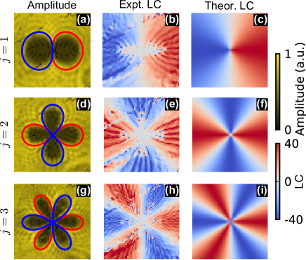
Figure 1: Multipoles of TC at $z=0$ cm. The rows correspond to the data for a dipole (a, b, c), quadrupole (d, e, f) and an hexapole (g, h, i). In columns we display the beam amplitude profiles (a,d,g), the experimental LC (b, e, h) and theoretical LC obtained from Eq. (7) (c, f, i). The solid lines in (a, d, g) corresponds to the expected OV core profile from Eq. (6), and their colors (red, blue) represent the enclosed TC sign (+, -).

An important property of TC multipoles is that their LC is stable under propagation, as can be seen by varying the position of the CCD along the $z$ axis. Experimental amplitude and LC at different values of $z$ are shown in Fig. 2 for $j=4$. It may be observed in the amplitude profiles, Figs. 2 (a-d), that pairs of amplitude lobes with opposed LC signs annihilate under propagation. The resulting bright spots are located at zero LC regions. Creation and annihilation of oppositely charged OV pairs under propagation are well established in literature Nye and Berry (1974); Indebetouw (1993); Roux (1995); Maleev and Swartzlander (2003), but to our knowledge the previous descriptions were always associated with, respectively, creation and destruction of TC. In the case we describe here, the beam’s topological structure is preserved under propagation, as can be seen from the LC in Fig. 2 (e-h). For negative $z$, the amplitude lobes rotate in the opposite direction to that shown in Figs. 2 (a-d).

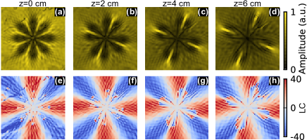
Figure 2: Propagation of a vortex octupole $\left(j=4\right)$ in free-space. In the top row (a-d) it is displayed the amplitude profile at increasing propagation distance from the SLM image plane $(z=0\mbox{ cm})$, while in the bottom row (e-h) is shown the experimental LC. Notice that the LC remains stable under propagation.

Another important property of the TP, Eq. (4), is that it satisfies a Gauss law inside a region $D$ for the total enclosed TC,

$$\oint_{\partial D}d\vec{l}\cdot\vec{\nabla}V\left(\mathbf{r}\right) =2\pi i\int_{D}da^{\prime}\rho\left(\mathbf{r}^{\prime}\right).$$ (9)

Equation (9) is a generalization of the usual expression for the winding number over the phase profile, where one would have $Q_{T}$ instead of $\int_{D}da^{\prime}\rho\left(\mathbf{r}^{\prime}\right)$ as the total TC enclosed by $\partial D$. However, since Eq. (9) was obtained from a continuum generalization, care must be taken in cases of continuous $\rho$. The discrete nature of TC makes $\rho$ an effective TC density.

To exemplify the meaning of $\rho$ in the continuous case we produced a radial distribution for simplicity. We consider that $\rho=\rho_{0}r^{n}$, where $\rho_{0}$ is constant, over a circle of radius $a$ and the total TC distributed is $Q_{T}$. Since now $\rho$ is distributed along a large region, the approximation of $r\sim 0$ is not valid, and the amplitude profile is not described by Eq. (6). However, the phase profile from Eq. (4) is always valid and equal to

$$\Phi_{T}=\begin{cases}Q_{T}\left[\left(\frac{r}{a}\right)^{n+2}\left(\phi-\pi\right)+\pi\right]&,\,r<a,\\ Q_{T}\phi&,\,r\geq a,\end{cases}$$ (10)

where we substituted $\rho_{0}=Q_{T}\left(n+2\right)/(2\pi a^{n+2})$ and it is assumed that $n\geq-2$.

Equation (10) is a generalization which smoothly connects usual OV $(n=-2)$ to helico-conical beams, or optical twisters Alonzo et al. (2005); Daria et al. (2011) in which $n=-1$. Optical twisters are interesting because they carry angular momentum and also have a higher photon density than the usual Laguerre-Gauss or Bessel beams Daria et al. (2011). Therefore they are of interest for manipulating particles Daria et al. (2011) and may also be of interest to nonlinear optics of OAM carrying beams Desyatnikov et al. (2005). To our knowledge, other values of $n$ were never previously reported in the literature.

We produced beams with the phase profile given by Eq. (10), with $Q_{T}=5$, fixed $a$ and varying $n$, and the results are shown in Fig. 3. In the phase profiles, Fig. 3(a-d), it can be seen that larger $n$ increase the phase twisting at $r<a$ and reallocates the TC towards the border along $\phi=\pi$. The TC displacement can be seen also in the zeros of the amplitude profiles, as shown in Fig. 3(e-h). The LC profiles, Fig. 3(i-l), shows that larger $n$ values decrease the LC near the center of the circle. In Fig. 3(m-p) we show the mean LC as a function of the radial distance to the center of the circle. The values obtained (black dots) agree with the theoretically expected from the phase profile (solid blue) via Eq. (10). The LC reduction in the center can be understood by considering that larger $n$ push $\rho$ to the boundaries of the circle $a$. Therefore the LC profile is directly associated with the $\rho$ distribution. Also, since the LC is proportional to the local classical OAM of the beam Amaral et al. (2014), this indicates that the classical OAM profile depends similarly on $\rho$.

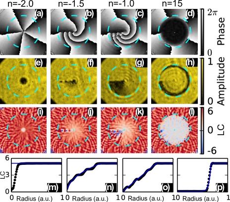
Figure 3: Data for 2D radial distribution, Eq. (10), with $Q_{T}=5$, fixed $a$ and varying $n$ (columns) at $z=0$ cm. $a$ is graphically represented by cyan dashed lines. The determined LC (black dots) at (m-p) corresponds to the azimuthally averaged LC at a given radial distance from the center of the circle as a function of the radial distance. The blue solid lines in (m-p) correspond to the values expected from the applied phase mask.

In summary, we introduced in this work the concept of the Topological Potential (TP), Eq. (4), by performing conformal transformations over screw dislocations Nye and Berry (1974). The identification of the TP paves the way for further understanding and tailoring of OV because it creates a bridge between OV and 2d electrostatics. For applications where the shape of an OV is relevant, as in optical tweezers Dholakia and Cizmár (2011), laser traps Jaouadi et al. (2010) or atom guides Rhodes et al. (2006), the TP might be used to design OVs for specific applications Amaral et al. (2013). Shaped OV may also allow selective excitation of plasmonic modes Brasselet et al. (2013). However, while the present work can be directly used for OV at the focus, further development is necessary to understand the effects of propagation and address issues as the stability of OV Abramochkin and Volostnikov (2004).

Another important point is that the discussed examples obtained from the TP might be useful in some applications. For instance, the intensity profile instability of TC multipoles may be used to determine the position of an extended object image plane, and in aligning spatial filters. Another possibility is that, since multipoles form a complete (Fourier) basis of orthogonal modes on the azimuthal phase, they may be suited for applications in quantum communications Vincenzo et al. (2012). In telecommunications, they are an alternative to Laguerre-Gauss beams for data multiplexing Wang et al. (2012) that can be more stable to turbulence Wang et al. (2012); Wang and Zheng (2009), since the topological information is distributed over the beam profile. The 2D TC distributions might be used to locally adjust the LC, and consequently the local OAM, of a light beam by calculating Eq. (4) analytically or numerically. This is specially interesting for optical tweezers, because then it becomes possible to locally adjust the light induced torques. Therefore, one may in principle control trapped particles in 2D by simply adjusting the TC distribution.

We acknowledge the financial support from the Brazilian agencies CNPq (INCT-Fotônica) and FACEPE. A. M. A. also acknowledge Tiago T. Saraiva for the helpful discussions.

References

- Xia et al. (2014) H. Xia, N. Francois, H. Punzmann, and M. Shats, Phys. Rev. Lett. 112, 104501 (2014).
- Scott and Dritschel (2006) R. K. Scott and D. G. Dritschel, J. Atmos. Sci. 63, 726 (2006).
- Abrikosov (2004) A. Abrikosov, Rev. Mod. Phys. 76, 975 (2004).
- Aranson and Kramer (2002) I. Aranson and L. Kramer, Rev. Mod. Phys. 74, 99 (2002).
- Yao and Padgett (2011) A. M. Yao and M. J. Padgett, Adv. Opt. Photon. 3, 161 (2011).
- Dennis et al. (2010) M. R. Dennis, R. P. King, B. Jack, O. Kevin, and M. J. Padgett, Nature Phys. 6, 118 (2010).
- Allen et al. (1992) L. Allen, M. W. Beijersbergen, R. J. C. Spreeuw, and J. P. Woerdman, Phys. Rev. A 45, 8185 (1992).
- Dholakia and Cizmár (2011) K. Dholakia and T. Cizmár, Nature Photon. 5, 335 (2011).
- Jaouadi et al. (2010) A. Jaouadi, N. Gaaloul, B. Viaris de Lesegno, M. Telmini, L. Pruvost, and E. Charron, Phys. Rev. A 82, 023613 (2010).
- Rhodes et al. (2006) D. P. Rhodes, D. M. Gherardi, J. Livesey, D. McGloin, H. Melville, T. Freegarde, and K. Dholakia, J. Mod. Opt. 53, 547 (2006).
- Brasselet et al. (2013) E. Brasselet, G. Gervinskas, G. Seniutinas, and S. Juodkazis, Phys. Rev. Lett. 111, 193901 (2013).
- Wang et al. (2012) J. Wang, J. Yang, I. M. Fazal, N. Ahmed, Y. Yan, H. Huang, Y. Ren, Y. Yue, S. Dolinar, M. Tur, and A. E. Willner, Nature Photon. 6, 488 (2012).
- Vincenzo et al. (2012) D. Vincenzo, E. Nagali, S. Walborn, L. Aolita, S. Slussarenko, L. Marrucci, and F. Sciarrino, Nature Comm. 3, 961 (2012).
- Nakahara (2003) M. Nakahara, Geometry, Topology and Physics (Taylor & Francis, 2003).
- Amaral et al. (2013) A. M. Amaral, E. L. Falcão-Filho, and C. B. de Araújo, Opt. Lett. 38, 1579 (2013).
- Amaral et al. (2014) A. M. Amaral, E. L. Falcão-Filho, and C. B. de Araújo, Opt. Express 22, 30315 (2014).
- Wang and Zheng (2009) L. Wang and W. Zheng, J. Opt. A: Pure Appl. Opt. 11, 065703 (2009).
- Pugatch et al. (2007) R. Pugatch, M. Shuker, O. Firstenberg, A. Ron, and N. Davidson, Phys. Rev. Lett. 98, 203601 (2007).
- Panofsky and Phillips (1962) W. K. H. Panofsky and M. Phillips, Classical Electricity and Magnetism (Addison-Wesley Publishing Company, 1962).
- Smythe (1950) W. R. Smythe, Static and Dynamic Electricity (McGraw-Hill Book Company, 1950).
- Nye and Berry (1974) J. F. Nye and M. V. Berry, Proc. R. Soc. Lond. A 336, 165 (1974).
- Note (1) Even our experimental beam having a flat-top amplitude profile, the Gaussian corresponds to the first correction to the condition near . Explicitly, .
- Curtis and Grier (2003) J. E. Curtis and D. G. Grier, Opt. Lett. 28, 872 (2003).
- Lin et al. (2005) J. Lin, X. Yuan, S. Tao, X. Peng, and H. Niu, Opt. Express 13, 3862 (2005).
- Abramochkin and Volostnikov (2004) E. G. Abramochkin and V. G. Volostnikov, Phys.-Usp. 47, 1177 (2004).
- Boivin et al. (1967) A. Boivin, J. Dow, and E. Wolf, J. Opt. Soc. Am. 57, 1171 (1967).
- Roux (1995) F. Roux, J. Opt. Soc. Am. B 12, 1215 (1995).
- Roux (2004) F. Roux, Opt. Commun. 236, 433 (2004).
- Berry (2004) M. V. Berry, J. Opt. A: Pure Appl. Opt. 6, 259 (2004).
- Leach et al. (2004) J. Leach, E. Yao, and M. J. Padgett, New J. Phys. 6, 71 (2004).
- Indebetouw (1993) G. Indebetouw, J. Mod. Opt. 40, 73 (1993).
- Maleev and Swartzlander (2003) I. Maleev and G. Swartzlander, J. Opt. Soc. Am. B 20, 1169 (2003).
- Alonzo et al. (2005) C. A. Alonzo, P. J. Rodrigo, and J. Glückstad, Opt. Express 13, 1749 (2005).
- Daria et al. (2011) V. R. Daria, D. Z. Palima, and J. Glückstad, Opt. Express 19, 476 (2011).
- Desyatnikov et al. (2005) A. S. Desyatnikov, A. A. Sukhorukov, and Y. S. Kivshar, Phys. Rev. Lett. 95, 203904 (2005).