Direct Measurement of Time-Frequency Analogues of Sub-Planck Structures

Abstract

Exploiting the correspondence between Wigner distribution function and a frequency-resolved optical gating (FROG) measurement, we experimentally demonstrate existence of the chessboard-like interference patterns with a time-bandwidth product smaller than that of a transform-limited pulse in the phase space representation of compass states. Using superpositions of four electric pulses as realization of compass states, we have shown via direct measurements that displacements leading to orthogonal states can be smaller than limits set by uncertainty relations. In the experiment we observe an exactly chronocyclic correspondence to the sub-Planck structure in the interference pattern appearing for superposition of two Schödinger-cat-like states in a position-momentum phase space.

It is the superposition principle that leads to interference and diffraction phenomena, determines evolution of wavepackets in classical and quantum systems. When applying to macroscopic objects, the interpretation paradox of wave function in superposition arises from Schrödinger’s gedanken experiment on cat states Schrodinger-cat . By a Schrödinger-cat-like state in quantum optics one usually understands a coherent superposition of two coherent states, say, $|\alpha\rangle+|-\alpha\rangle$. Experimentally, such superpositions were created, e.g., in the atomic and molecular systems ion ; Haroche , superconducting circuits supQbits ; Wal , and quantum optical setups Ourjoumtsev-1 ; Tak . It has been noted by Zurek Zurek that a superposition of two Schrödinger-cat-like states (four coherent states in total, $|\alpha\rangle+|-\alpha\rangle+|i\alpha\rangle+|-i\alpha\rangle$, a so called compass state) in a Wigner phase-space description wigner1932 gives rise to the interference structure changing rapidly on an area smaller than a Planck’s constant $\hbar$. The result is counterintuitive because the Heisenberg’s uncertainty principle sets a limitation on the simultaneous resolutions in two conjugate observables.

It turns out that the sub-Planck structure determines scales important to the distinguishability of quantum states Zurek , thereby, potentially has an impact on an ultra-sensitive quantum metrology ion-trap ; Toscano and could affect efficient storage of quantum information entangle-2 ; Science . In principle, these sub -Planck structures could be used to improve the sensitivity in weak-force detection Roy ; weak and to help maintaining a high fidelity in the continuous-variable teleportation protocols decay ; teleportation . In practice, the classical wave optics analogues of sub-Planck structures in time-frequency domain were observed experimentally so far only for superposition of two Gaussian pulses Ludmila ; Walmsley . Obviously, a single Schrödinger-cat-like state offers a sensitivity to the perturbations only in one direction: perpendicularly to the line joining the coherent states. To provide sensitivity in all directions, another pair of coherent states is needed. Theoretical proposals for generation of compass states include interaction in cavity-QED systems GSA-PRA ; Science , evolution in a Kerr medium Tanas ; Magda and fractional revivals of molecular wavepackets Ghosh . Nevertheless, there was no experimental proof in the more complex and demanding case of superposition of four pulses. The main technical challenge in the preparation of states separated simultaneously in two conjugate coordinates comes from the difficulty in keeping the coherence among them. Furthermore, performing measurements of such tiny phase space structures is far from trivial.

In this Letter, we report a direct measurement of a compass state superposition of four optical pulses and the corresponding interference pattern in the time-frequency domain. The mathematical equivalence between the electric field of an ultrashort pulse and the quantum mechanical wave function of the same shape, enables us to observe the phase space structures through the time-dependent spectrum of light. The experimental data obtained from frequency-resolved optical gating (FROG) measurements of light pulses reveals sub-Planck structure analogues corresponding directly to the compass states. In the interference patterns, areas smaller than that of transform-limited pulses are measured, illustrating that displacements leading to orthogonality of compass states can be smaller than the Fourier limit imposed on the pulses forming these superpositions.

As illustrated in Fig. 2(b), in our second-harmonic generation (SHG) FROG measurement frog-book the input optical pulse $E(t)$ is split into two replicas with a tunable time delay by passing through a standard Michelson interferometer. These two mutually delayed replicas mix in a $\chi^{(2)}$ nonlinear crystal such as the Barium borate (BBO) crystal used in our experiment. Then, a spectrally resolved sum frequency signal is recorded for each time delay $\tau$. The resulting time-frequency map (spectrogram) implemented by the nonlinear self-optical gating mechanism can be formulated as the following function for an initial field $E(t)$:

$$\mathcal{I}^{\text{FROG}}_{\text{E}}(\tau,\omega)=\biggl{|}\int_{\scriptscriptstyle{-\infty}}^{\scriptscriptstyle{\infty}}\!\!\!\!E(t)\,E(t-\tau)\,e^{i\omega t}\,dt\biggl{|}^{2}.$$ (1)

For pulses with real envelopes and a linear phase, the spectrogram (1) is easily mapped to the Wigner quasi-probability distribution $W(q,p)$ wigner1932 :

$$W(q,p)=\frac{1}{\pi\hbar}\int_{-\infty}^{\infty}\,e^{2i\xi p/\hbar}\,F(q-\xi){F}^{\ast}(q+\xi)\,d\xi,$$ (2)

as

$$\mathcal{I}^{\text{FROG}}_{\text{E}}(\tau,\omega)\propto\big{|}W(\tau/2,\omega/2)\big{|}^{2}.$$ (3)

Here, ${F}^{\ast}(q)$ denotes the complex conjugate of $F(q)$, $\hbar$ is set to $1$, and our time and frequency domains are represented by $(\tau,\omega)$. Moreover, under these conditions, all cross-sections of the FROG spectrogram correspond to a scalar product between the probe state $E(t)$ and its ‘twin’ appropriately shifted in time or frequency chirp ; Ludmila . Thus, zeros of the cross-sections appear for these values of time and frequency shifts that lead to orthogonal states. In the following, we check the scale of the phase space displacements resulting in distinguishable states based on this property. Let us stress that the data presented here comes from direct spectrogram measurements and, unlike typical FROG applications, does not involve steps of state reconstruction.

In our experiment, an Er-doped fiber laser with $1564\,$nm center wavelength, $37\,$nm spectral bandwidth and $5.68\,\mathrm{MHz}$ repetition rate is used as the light source. To construct a compass state, i.e., the superposition of four coherent states, a pulse shaper is introduced to split the input pulse in both time and frequency domains, as illustrated in Fig.2(a) C-C . Here, a telescope is employed to improve the spectral resolution of the pulse shaper by expanding the beam diameter from $2.8\,\mathrm{mm}$ (at the collimator) to $4.5\,$mm. The input pulse is directly shaped in frequency domain, though a set of grating, lens, and a spatial light modulator (SLM). The whole spectrum occupies $320$ pixels in the SLM, and the throughput of our pulse shaper is around $30$%. The spectral separation is realized by blocking the central range of the input spectrum, see Fig. 2(a); while the temporal separation $2t_{0}$ is achieved by imposing an extra mask function $M_{\text{SLM}}(\omega)=\cos(\omega t_{0})e^{-i\omega t_{0}}$ via the SLM opt . The spectrally and temporally separated coherent pulses are further made transform limited by compensating the residual spectral phase via the phase modulation function of the pulse shaper. The power spectrum and temporal intensity of an example are shown in Figs. 2(a) and  2(b), respectively. In total, an initial laser spectra was divided into four pulses separated simultaneously by $2\omega_{0}$ in frequency and $2t_{0}$ in time, i.e., shaped into our time-frequency representation of the compass state. For practical reasons, in the experiment separation between pulses in frequency was kept constant while time separation $2t_{0}$ varied from $1.5\,$ps to $5\,$ps.

In the ideal case, when the pulses cut from the initial laser spectrum have Gaussian envelopes, the state generated in a pulse shaper has the form

$$E_{\text{in}}(t) \simeq e^{-(t-t_{0})^{2}-i(\omega-\omega_{0})t}+e^{-(t+t_{0})^{2}-i(\omega-\omega_{0})t}$$ (4)

$$+ e^{-(t-t_{0})^{2}-i(\omega+\omega_{0})t}+e^{-(t+t_{0})^{2}-i(\omega+\omega_{0})t},$$

(b)  

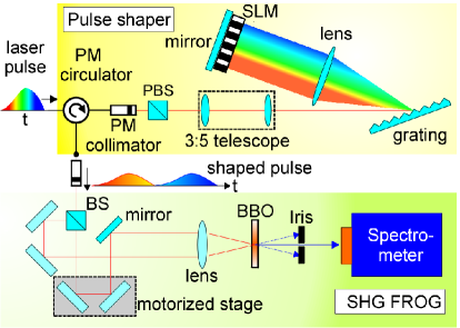
(a)

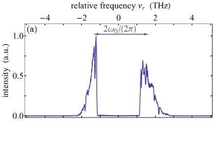
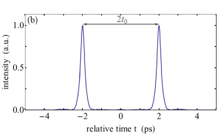
Figure 1: (Color online) Schematic view of our experimental setup, including (a) Pulse shaper composited of a set of grating, lens, and spatial light modulator (SLM); (b) SHG FROG composited by a beam splitter (BS) and a motorized stage in one arm to control time delay $\tau$, a nonlinear crystal (BBO) for the second harmonic generation (SHG), and a spectrometer.

Figure 2: Typical experimental profiles for our compass states are shown as a function of (a) relative frequency $\nu_{r}=\omega/(2\pi)$ and (b) time $t$. Here, the four pulses are concurrently separated by $\omega_{0}/\pi=3.3\,$THz in frequency and $2t_{0}=4\,$ps in time.

where $2t_{0}$ and $2\omega_{0}$ are the time and frequency separations between the Gaussian peaks. For the clarity of notation, normalization coefficients and parameters denoting width of the wavepackets are omitted in Eq. (4). Depending on the context, in the text that follows we will use either a regular frequency $\nu$ or the corresponding angular frequency $\omega=2\pi\nu$. The compass state $E_{\text{in}}(t)$ from Eq. (4) is constructed as a superposition of two mutually delayed pairs of pulses with the same carrier frequency in each pair; it corresponds to the original compass state from Zurek paper Zurek rotated by $\pi/{4}$ in the phase space.

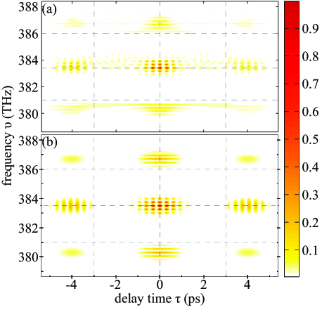
Figure 3: (Color online) Compass state in the phase space obtained by (a) FROG map measured for $t_{0}=2$ps; and (b) numerical simulation calculated for a superposition of four perfect identical Gaussian pulses.

A comparison between a theoretical simulation and experimentally obtained time and frequency phase space maps of compass states is presented in Fig. 3, where spectrograms corresponding to the same time and frequency separation between the cat states are plotted. Experimental data from SHG FROG spectrogram measured for $t_{0}=2\,$ps is shown in Fig. 3(a); while the theoretical plot calculated analytically for perfect Gaussian pulses is presented in Fig. 3(b). In addition to four peaks representing Gaussian wavepackets and located at the four corners of the plots, characteristic patterns of interference fringes are clearly visible between every two of the peaks. Moreover, in the center of four perimeters, a chessboard-like interference pattern appears. In the following, we will verify that for large enough separation between the peaks this chessboard-like pattern is constructed from areas smaller than $\Delta\tau\Delta\omega=1/2$ indicated by uncertainty relation, which would correspond to sub-Planck areas in the position-momentum phase space. For the shape of our pulses is obtained by cutting the laser spectra, a slight discrepancy between the patterns formed by the real experimental profiles and theoretically considered ideal Gaussian pulses can be seen between Figs. 3(a) and 3(b).

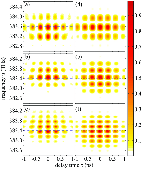
Figure 4: (Color online) Zooms of the central interference structure of FROG maps measured for (a) $t_{0}=1.25$ps, (b) $t_{0}=1.75$ps, and (c) $t_{0}=2.5$ps. As a comparison, the corresponding simulations calculated for compass states build from perfect Gaussian pulses are shown in (d), (e), and (f), respectively.

In the Wigner representation of a compass state, the middle interference pattern is build up from small rectangles of alternating positive and negative values of the function. Even though recordings in the FROG spectrograms take on only non-negative values, areas of the above-mentioned rectangles remain the same, i.e., the distances between subsequent zero lines do not change. For a large enough separation distances between pulses forming the superposition, these areas grow smaller than the area unit defined by the elementary uncertainty relation. In quantum mechanical version, the area unit is equal to $\hbar/2$; while in a chronocyclic phase space, it is simply $1/2$. It is worth noting that even for smaller separation distances “sub-Fourier” areas might appear in the FROG maps, namely, the areas smaller than those corresponding to dispersion $\Delta\tau\Delta\omega$ calculated for any from the pulses forming the compass state superposition. To demonstrate how the interference structure appearing in the middle of FROG maps changes with change of initial parameters, in Fig. 4, zooms of the central parts of spectrograms for different time separations between pair of pulses are presented. Figure 4 shows the Zoom of the central interference patterns obtained from the FROG traces for (a) $t_{0}=1.25\,$ps, (b) $t_{0}=1.75\,$ps, and (c) $t_{0}=2.5\,$ps. The corresponding theoretical plots made for superpositions of four identical Gaussian pulses are shown in in Figs. 4(d), (e), and (f), respectively. The comparison serves to illustrate that areas between zero lines of FROG maps indeed decrease with an increasing separation between pair of pulses. Again, as due to imperfections, amplitudes of pulses used in the experiment were not the same and the resulting interference patterns measured are not symmetric in respect to the central wavelength line.

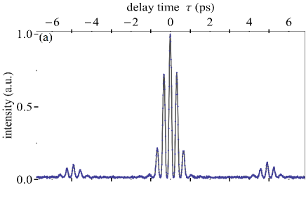
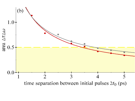
Figure 5: (Color online) (a) A central frequency ($\nu=383.36\,$THz) cross-section of the FROG map measured for $t_{0}=2.5\,\mathrm{ps}$. Here, blue dots depict measured intensity values for a given time delay $\tau$ introduced between two input state copies in the arms of FROG apparatus. (b) Average areas, $\Delta\tau\Delta\omega$, of the rectangles appearing between the zero lines in the interference structure of the central part of FROG maps. Values depicted by red or gray dots correspond to two independent sets of experimental data, respectively. Region below the uncertainty relation limit of $0.5$ is denoted in yellow.

Finally, let us examine the cross-section of the FROG map measured for $t_{0}=2.5\,$ps along the central wavelength $\lambda=782\,$nm ($\nu=383.36\,$THz) presented in Fig. 5(a). As mentioned before, the cross-sections of FROG spectrograms give values of the scalar product of a probe field with its ideal copy, but shifted in phase space in a direction perpendicular to the direction defining the cross-section. It is clearly seen that the values of the function plotted in Fig. 5(a) decrease to zero between the subsequent peaks. A time shift equal to one half of the distance between the zeros results in the superpositions orthogonal to the initial compass state. This result is complementary to the one reported in Ref. Ludmila , where zeros in cross-sections defined by $\tau=0$ were shown. Figure 5(b) demonstrates how average areas $\Delta\tau\Delta\omega$ of individual rectangles forming the central interference pattern, change with the change of parameter $t_{0}$. The average values of $\Delta\tau\Delta\omega$ plotted in Fig. 5(b) are calculated for two independently collected sets of data (depicted by gray or red dots, respectively). These two sets of data are measured for slightly different pulse shapes and differently set time delay resolution, i.e., different values of the smallest stage-motor step. It is clearly seen that in both cases for larger separation distances, areas between zeros indeed reach below limit imposed by uncertainty relation. Exactly these areas determine a scale of smallest change ensuring distinguishability of the mutually shifted states. As a last point, we would like to underline that the uncertainty relation is not violated. What we prove here is that a sub-Fourier change of initial state (shift in frequency and/or time) is enough to produce state orthogonal to the initial superposition. In the quantum mechanics this leads to a perfect distinguishability of states.

In summary, using correspondence between FROG maps in a chronocyclic phase space and the Wigner distribution function, we have demonstrated existence of the interference structure changing on areas smaller than that of a transform-limited pulse. We have performed FROG measurements of compass states realized through superpositions of four light pulses constructed with a help of a spatial light modulator (SLM), by manipulating the phase difference in the spectrum. Interpretation of the FROG spectrograms as maps of the values of a scalar product between probe pulses and their shifted copies, allowed us to show explicitly that the scale of changes leading to orthogonality of states indeed goes below the Fourier limit if sufficient time and frequency separations are simultaneously kept between the input pulses. The sub-Planck structure of the interference pattern in phase space representation of compass states not only manifests itself as a generalized Schödinger’s cat state, but also provides the platform to exploit quantum metrology and quantum information processing through ultrafast optics.

This work is supported in part by the Ministry of Science and Technologies, Taiwan, under the contract No. 101-2628-M-007-003-MY4, No. 103-2221-E-007-056, and No. 103-2218-E-007-010.

References

- (1) E. Schrödinger, “Die gegenwartige Situation in der Quantenmechanik”, Naturwissenschaften 23, 807 (1935); ibid. 23, 823 (1935); ibid. 23, 844 (1935).
- (2) C. Monroe, D. Meekhof, B. E. King, and D. J. Wineland, “A “Schrödinger cat” superposition state of an atom,” Science, 272, 1131 (1996).
- (3) M. Brune, E. Hagley, J. Dreyer, X. Maître, A. Maali, C. Wunderlich, J. M. Raimond, and S. Haroche, “Observing the progressive decoherence of the “Meter” in a quantum measurement,” Phys. Rev. Lett. 77, 4887 (1996).
- (4) J. R. Friedman, V. Patel, W. Chen, S. K. Tolpygo, and J. E. Lukens, “Quantum superposition of distinct macroscopic states,” Nature 406, 43 (2000).
- (5) C. H. van der Wal, A. C. J. ter Haar, F. K. Wilhelm, R. N. Schouten, C. J. P. M. Harmans, T. P. Orlando, S. Lloyd, and J. E. Mooij, “Quantum superposition of macroscopic persistent-current states,” Science 290, 773 (2000).
- (6) A. Ourjoumtsev, R. Tualle-Brouri, J. Laurat, and P. Grangier, “Generating optical Schrödinger kittens for quantum information processing,” Science 312, 83 (2006);
- (7) H. Takahashi, K. Wakui, S. Suzuki, M. Takeoka, K. Hayasaka, A. Furusawa, and M. Sasaki, “Generation of large-amplitude coherent-state superposition via ancilla-assisted photon-subtraction,” Phys. Rev. Lett. 101, 233605 (2008).
- (8) W. H. Zurek, “Sub-Planck structure in phase space and its relevance for quantum decoherence,” Nature 412, 712 (2001).
- (9) E. Wigner, “On the Quantum Correction For Thermodynamic Equilibrium”, Phys. Rev. 40, 749 (1932).
- (10) D. A. R. Dalvit, R. L. de Matos Filho, and F. Toscano, “Quantum metrology at the Heisenberg limit with ion trap motional compass states,” New J. Phys. 8, 276 (2006).
- (11) F. Toscano, D. A. R. Dalvit, L. Davidovich, and W. H. Zurek, “Sub-Planck phase-space structures and Heisenberg-limited measurements,” Phys. Rev. A 73, 023803 (2006).
- (12) J. R. Bhatt, P. K. Panigrahi, and M. Vyas, “Entanglement induced sub-Planck structures,” Phys. Rev. A 78, 034101 (2008).
- (13) B. Vlastakis, G. Kirchmair, Z. Leghtas, S. E. Nigg, L. Frunzio, S. M. Girvin, M. Mirrahimi, M. H. Devoret, and R. J. Schoelkopf, “Deterministically encoding quantum information using 100-photon Schrödinger cat states,” Science 342, 697 (2013).
- (14) U. Roy, S. Ghosh, P. K. Panigrahi, and D. Vitali, “Sub-Planck-scale structures in the Pöschl-Teller potential and their sensitivity to perturbations,” Phys. Rev. A 80, 052115 (2009).
- (15) J. Dressel, C. J. Broadbent, J. C. Howell, and A. N. Jordan, “Experimental violation of two-party Leggett-Garg inequalities with semiweak measurements,” Phys. Rev. Lett. 106, 040402 (2011).
- (16) Ph. Jacquod, I. Adagideli, and C. W. J. Beenakker, “Decay of the Loschmidt echo for quantum states with sub-Planck-scale structures,” Phys. Rev. Lett. 89, 154103 (2002).
- (17) A. J. Scott and C. M. Caves, “Teleportation fidelity as a probe of sub-Planck phase-space structure,” Ann. Phys. 323, 2685, (2008).
- (18) L. Praxmeyer, P. Wasylczyk, Cz. Radzewicz, and K. Wódkiewicz, “Time-frequency domain analogues of phase space sub-Planck structures,” Phys. Rev. Lett. 98, 063901 (2007).
- (19) D. R. Austin, T. Witting, A. S. Wyatt, and I. A. Walmsley, “Measuring sub-Planck structural analogues in chronocyclic phase space,” Opt. Comm. 283, 855 (2010).
- (20) G. S. Agarwal and P. K. Pathak, “Mesoscopic superposition of states with sub-Planck structures in phase space,” Phys. Rev. A 70, 053813 (2004).
- (21) R. Tanaś, “Nonclassical states of light propagating in Kerr media” in Theory of Non-classical States of Light, V. Dodonov and V. I. Mańko eds., (Taylor and Francis, 2003).
- (22) M. Stobińska, G.J. Milburn, and K. Wódkiewicz, “Wigner function evolution of quantum states in the presence of self-Kerr interaction,” Phys. Rev. A 78, 013810 (2008).
- (23) S. Ghosh, A. Chiruvelli, J. Banerji, and P. K. Panigrahi, “Mesoscopic superposition and sub-Planck-scale structure in molecular wave packets,” Phys. Rev. A 73, 013411 (2006); S. Ghosh, U. Roy, C. Genes, and D. Vitali, “Sub-Planck-scale structures in a vibrating molecule in the presence of decoherence,” Phys. Rev. A 79, 052104 (2009).
- (24) R. Trebino, “Frequency-Resolved Optical Gating: the measurement of ultrashort laser pulses,” (Springer, 2002).
- (25) L. Praxmeyer, and K. Wódkiewicz, “Time and frequency description of optical pulses,” Laser Phys. 15, 1477, (2005).
- (26) C.-C. Chen and S.-D. Yang, “All-optical self-referencing measurement of vectorial optical arbitrary waveform,” Opt. Express 22, 28838 (2014).
- (27) C.-S. Hsu, H.-C. Chiang, H.-P. Chuang, C.-B. Huang, and S.-D. Yang, “Forty-photon-per-pulse spectral phase retrieval by modified interferometric field autocorrelation,” Opt. Lett. 36, 2611 (2011).