A Herschel/HIFI Legacy Survey of HF and H₂O in the Galaxy:
Probing Diffuse Molecular Cloud Chemistry

Abstract

We combine Herschel observations of a total of 12 sources to construct the most uniform survey of HF and H₂O in our Galactic disk. Both molecules are detected in absorption along all sight lines. The high spectral resolution of the Heterodyne Instrument for the Far-Infrared (HIFI) allows us to compare the HF and H₂O distributions in 47 diffuse cloud components sampling the disk. We find that the HF and H₂O velocity distributions follow each other almost perfectly and establish that HF and H₂O probe the same gas-phase volume. Our observations corroborate theoretical predictions that HF is a sensitive tracer of H₂ in diffuse clouds, down to molecular fractions of only a few percent. Using HF to trace H₂ in our sample, we find that the $N$(H₂O)-to-$N$(HF) ratio shows a narrow distribution with a median value of 1.51. Our results further suggest that H₂O might be used as a tracer of H₂ -within a factor 2.5- in the diffuse interstellar medium. We show that the measured factor of $\sim$2.5 variation around the median is driven by true local variations in the H₂O abundance relative to H₂ throughout the disk. The latter variability allows us to test our theoretical understanding of the chemistry of oxygen-bearing molecules in the diffuse gas. We show that both gas-phase and grain-surface chemistry are required to reproduce our H₂O observations. This survey thus confirms that grain surface reactions can play a significant role in the chemistry occurring in the diffuse interstellar medium ($n_{\rm H}$ $\leq$1000 cm^-3).

1 Introduction

Diffuse molecular clouds are regions in which atomic hydrogen is progressively converted to molecular hydrogen (H₂), and neutral carbon and carbon monoxide become the dominant forms of carbon as the total visual extinction increases from 0.1 (the onset of H₂ formation) to about 2 magnitudes (see, Snow & McCall 2006, for a review). Diffuse molecular clouds are considered clouds in transition from diffuse mainly atomic gas to fully molecular gas, hence an important first step in star formation. As a result, they play a crucial role in the lifecycle of the interstellar medium making their study critical to advance our understanding of how molecular clouds form from the diffuse interstellar medium (ISM).

Because of their relatively low densities ($n_{\rm H}$ $\leq$1000 cm^-3) and their low shielding from UV radiation compared to dense clouds, diffuse molecular clouds were expected to be mostly devoid of molecules. However, the last four decades of UV/optical/radio observations, from space and from the ground, have demonstrated that diffuse molecular clouds have a surprisingly rich and still largely unexplained chemistry (e.g., Snow & McCall 2006, Sonnentrucker et al. 2007; Sheffer et al. 2008; Liszt et al. 2007; Neufeld et al. 2012). Comparisons of UV/optical molecular absorption line studies with high-resolution studies using sub-mm data have provided complementary information on the physics and chemistry of the absorbing gas, over a large range of opacities and at great distances in the Galactic disk. As a result, these clouds constitute “in-situ” laboratories in which we can study a variety of physical and chemical processes of broad applicability in astrophysics.

Small (diatomic and triatomic) hydrides are important tracers of the diffuse interstellar medium physics and chemistry. Possessing small moments of inertia, these hydrides have rotational transitions at THz frequencies that are difficult or impossible to observe using ground-based observatories. The Herschel/HIFI Key Program PRISMAS (Probing InterStellar Molecules with Absorption line Studies: PI, M. Gerin) was aimed at surveying key hydrides within the Galaxy. Up to 22 small molecular species were specifically targeted with PRISMAS in order to probe the chemistry of carbon (e.g., Mookerjea et al. 2010, Gerin et al. 2010, Godard et al. 2012; 2014), nitrogen (e.g., Persson et al. 2010; Persson et al. 2014), oxygen (e.g., Neufeld et al. 2010; Flagey et al. 2013; Indriolo et al. 2015), chlorine (e.g., Lis et al. 2010; De Luca et al. 2012; Neufeld et al. 2012, Monje et al. 2013) and fluorine (e.g., Neufeld et al. 2010, Sonnentrucker et al. 2010; this paper) in diffuse molecular clouds and to constrain the physical processes at play in the Galactic diffuse ISM.

In this work, we focus on two particular hydrides, hydrogen fluoride (HF) and water (H₂O) with the aim of further probing the chemistries of fluorine and oxygen-bearing molecules and of determining to what extent both species can be used as diagnostics of the physical processes at play in the diffuse ISM. The combination of the full PRISMAS sample, with some WISH data (Water In Star-forming regions with Herschel; PI: E. F. van Dishoeck) and Herschel Cycle 1 data allows us to report on the largest set of HF and H₂O column density measurements in the Galactic disk to-date. Sections 2 & 3 describe our set of observations, as well as the reduction and analysis techniques we employed. Section 4 summarizes our results. In Sections 5 & 6 we compare the HF and H₂O distributions measured with our survey to the most recent 2-sided PDR model predictions (Neufeld & Wolfire 2009, Hollenbach et al. 2012) for the range of physical conditions most relevant to diffuse molecular clouds. In particular, we validate the role of HF as a tracer of H₂ and add weight to the suggestion that H₂O can be used as a tracer of H₂ in diffuse clouds as well (e.g., Flagey et al. 2013). We confirm the co-spatial distribution of HF and H₂O in the Galactic diffuse ISM, which in turn allows us to derive the H₂O abundance relative to HF throughout the Galactic disk. In Section 7 we discuss how the measured variations in the H₂O abundance relative to HF can be used to test our understanding of the H₂O chemistry. We assert the role that grain surface chemistry plays in the production of H₂O in the diffuse interstellar medium. Section 8 summarizes our general conclusions.

2 Observations

The names and coordinates of the 12 targets comprising our sample are summarized in Table 1. All targets are well-studied star-forming regions, known to produce strong far-infrared background continuum emission, a prerequisite for detecting absorption by foreground interstellar clouds. The sight lines to each of these sources are also known to intersect multiple spiral arms, hence, allowing us to probe a variety of local physical conditions throughout the Galactic disk (e.g., Godard et al. 2010; Lang et al. 2010). The sources G$-$0.02$-$0.07 ($+$50 km s^-1 cloud around SgrA), G$-$0.13$-$0.08 ($+$20 km s^-1 cloud around SgrA), W28A, W31C, W33A, G34.3$+$0.1, W49N, W51, W3 IRS5 and DR21(OH) were observed through Guaranteed Time Key Program PRISMAS. W3 IRS5 was also observed in Guaranteed time Key Program WISH. W3(OH) and G29.96$-$0.02 were observed as part of the Herschel Open Time Cycle 1 campaign (OT1, PI: D.A. Neufeld) along with W51 that was reobserved to significantly increase our signal-to-noise (S/N) ratio in the continuum and push our detection limits to lower column density clouds compared to those measured from data previously obtained with the PRISMAS program.

We observed the ground-state rotational line of HF ($\nu_{\rm rest}=$ 1232.476 GHz; Nolt et al. 1987) in the upper sideband of HIFI band 5a receiver and the ground-state line of para-H₂O (p-H₂O; $\nu_{\rm rest}=$ 1113.343 GHz) in the lower sideband of HIFI band 5a receiver. We used multiple Local Oscillator (LO) settings in order to securely identify the HF and p-H₂O absorption lines along all 12 sight lines. The proximity of the HF and p-H₂O lines in frequency and their detection within the same receiver band ensure that the absorption lines are observed with a very similar telescope performance and that the data are calibrated in a similar fashion.

We used the Dual Beam Switch (DBS) mode which, combined with the Wide Band Spectrometer (WBS), allows for a spectral resolution of about 1.1 MHz (0.3 km s^-1 at the HF frequency). The DBS mode uses two reference OFF-beam positions located 3$\arcmin$ on either side of the source position, along an East-West axis. Because the Galactic Center is a very complex and crowded region, we checked for emission or absorption (contamination) in the OFF-beam position using Herschel observations performed by the HEXGAL project (R. G$\ddot{\hbox{u}}$sten and M. Requena-Torres, private communication). There is no contamination at the OFF-beam position for HF; only minor contamination occurs for p-H₂O in the velocity range [$-$ 40, $+$10] km s^-1. As a result, the absorption components detected in the Galactic disk in this particular velocity range are not included in the analysis described in Section 3 for the two Galactic Center sources G$-$0.02$-$0.07 and G$-$0.13$-$0.08. Contamination in the OFF-beam position is not a concern for the remaining more compact sources in our sample.

3 Data Reduction and Analysis

The data were processed to Level 2 with the standard HIFI pipeline in the Herschel Interactive Processing Environment (HIPE) version 9.1 (Ott 2010), thereby producing fully calibrated spectra for both polarization modes at each LO setting. Further inspection of the Level 2 data showed that the signals obtained in each of the two polarization modes for a given LO setting were in excellent agreement, as were the HF and p-H₂O spectra obtained at each LO setting. Occasionally, emission from molecules other than HF or p-H₂O appear in the sideband containing the HF or p-H₂O absorption (see Fig 1). For 6 of the 12 sources presented here, Flagey et al. (2013) performed a detailed study of the distribution of water in the ground and excited states accessible to Herschel/HIFI. While contamination needed to be taken into account for some of the excited states of water, their study showed that the ground-state of p-H₂O, of interest here, was mostly free of this effect. For the remaining 6 sources in our sample we compared the absorption profiles of the ground states of HF and p-H₂O across LO settings and for both polarizations. Our comparisons revealed no significant contamination with interloping features for both molecules. As a result, for each target, we generated average spectra for HF and p-H₂O that consist of the weighted sum of up to 6 spectral observations (up to three LO settings with two polarizations each), for which each observation is weighted in inverse proportion to the square of its root mean square (rms) noise. The double sideband continuum antenna temperatures T_A(cont) and respective rms noise for HF and p-H₂O derived from these weighted average spectra are reported in Table 2, which also lists the total on-source exposure times (t_exp), the observation dates, and the observation IDs (Obs IDs) of the LO settings obtained for HF and p-H₂O.

3.1 Background Continuum Emission Treatment

HIFI employs double sideband receivers and for a sideband gain ratio equal to unity, the saturated absorption of radiation at a given frequency for a transition with excitation temperature much less than T_A(cont) will reduce the measured antenna temperature (T_A) to one-half the apparent continuum antenna temperature T_A(cont).

The top two panels of Figures 1 through 6 display the double sideband weighted average spectra for HF and p-H₂O, respectively, versus Doppler velocity in the Local Standard of Rest frame (V_LSR) for each of the 12 sight lines probed in our survey. For most sight lines, HF is detected only in absorption, and the background continuum emission from the source itself is well modeled with a constant (red line in each panel). The flux normalized with respect to the continuum flux in a single sideband can then be expressed as,

T_A/T_A(cont) = (1/2)[1 + $$\exp -\tau$$()]

assuming that the sideband gain ratio is equal to unity. The latter assumption was investigated by Flagey et al. (2013) who found that the HIFI sideband gain ratio in band 5a, the band of interest here, was very stable and indeed consistent with unity.

Toward W31C, W3 IRS5, W28A and W49N, one can see that HF emission arising from gas local to the star-forming region blended itself with HF absorption arising from foreground clouds with projected velocities similar to those of the emitting gas. Such blending also occurs for the p-H₂O line absorption toward almost all the sight lines surveyed here. In these cases, we treated the HF and p-H₂O emission as features confined to the proximity of the background continuum sources and modeled them as an additional background continuum emission that adds to the dust emission, as was done in Flagey et al. (2013). For these sight lines, we adopted a linear combination of a zeroth-order polynomial and up to 3 Gaussian profiles to model the shape of the observed background over the regions unaffected by blending with the foreground absorption. In Figs. 1-6, we plotted our best fit models in red over the double sideband spectra of HF and p-H₂O (black lines) for the velocity regions that can be constrained by our data. Since the H₂O emission profiles were constrained using the 1113 GHz features alone, our continuum emission models are not as robust as those obtained by Flagey et al. (2013). As a result, the velocity ranges significantly affected by these continuum emission features are not discussed further here and are not displayed in the bottom two panels of Figs. 1-6.

Assuming a sideband gain ratio equal to unity, the flux normalized with respect to the continuum flux in a single sideband is then expressed as

$$\hbox{$\exp$($-\tau$)=[T${}_{A}$/T${}_{A}$(cont) $-$ 0.5]/[T${}_{e}$/T${}_{A}$(cont) $+$ 0.5]},$$

where T_e is the continuum emission arising from the HF or p-H₂O -containing gas proximate to the star-forming regions and T_A corresponds to the absorption due to the diffuse ISM foreground gas of interest for this study. The middle panels in Figs. 1-6 display the resulting single sideband, continuum normalized spectrum for HF (black line) and p-H₂O (blue line) versus V_LSR for our sample. The horizontal black lines represent the continuum temperature normalized to unity and the zero flux level. One can see that toward all sources, the sideband gain ratios are indeed consistent with unity within our uncertainties (see Table 2).

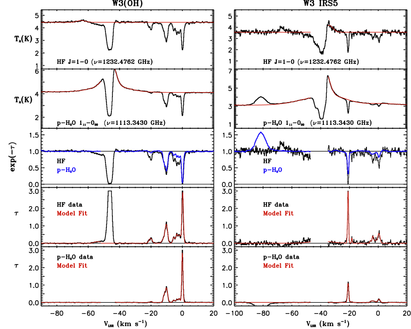
Figure 1: Top two panels: Double sideband $rms$-weighted average spectra for HF and p-H₂O versus Doppler velocity in the Local Standard of Rest frame (V_LSR) toward W3 IRS5 (right) and W3(OH) (left). The best fit model to the background continuum plus line emission is overlaid in red. The velocity range over which the foreground HF absorption or the foreground p-H₂O absorption is blended with emission proximate to the background source is excluded from the modeling. Middle panel: Single sideband continuum normalized spectra for HF (black line) and p-H₂O (blue line). The velocity range in which blending occurs is not plotted. Bottom two panels: Optical depth profiles for HF and p-H₂O (black lines) versus V_LSR, respectively. Overlaid in red are the best multi-Gaussian fit models for the HF and p-H₂O profiles for the gas components detected in the foreground of each source that do not suffer saturation.

Figure 2: Same as in Figure 1 for G$-$0.02$-$0.07 ($+$50 km s^-1 cloud around SgrA, left) and G$-$0.13$-$0.08 ($+$20 km s^-1 cloud around SgrA, right).

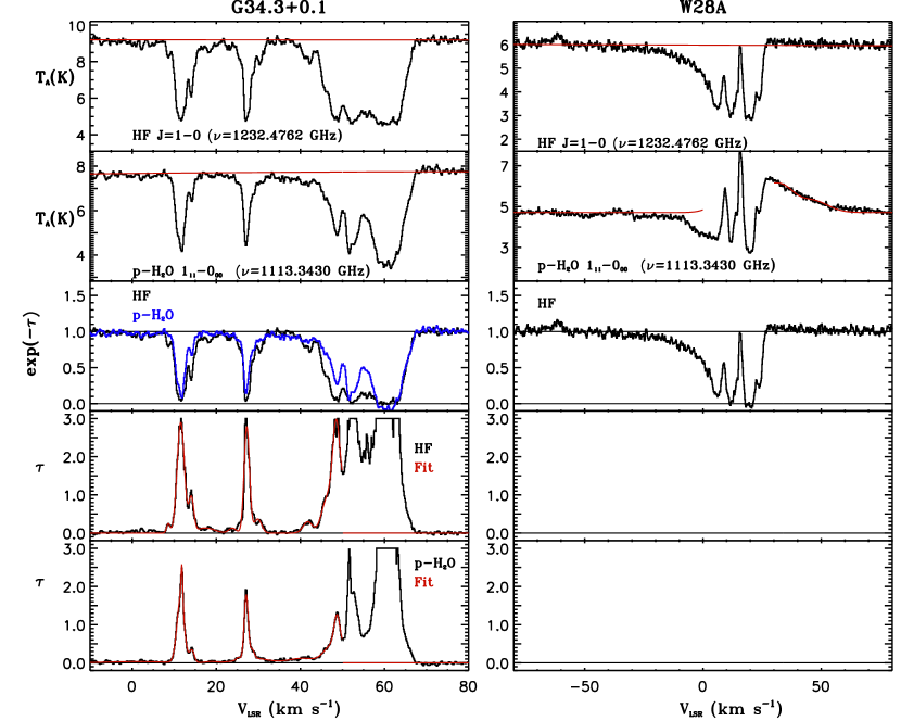
Figure 3: Same as in Figure 1 for G34.3$+$0.1 (left). In the case of W28A (right), the velocity ranges of the foreground absorption and the background emission for HF and p-H₂O coincide. As a result, the optical depth profiles and corresponding multi-component Gaussian fits are not presented here.

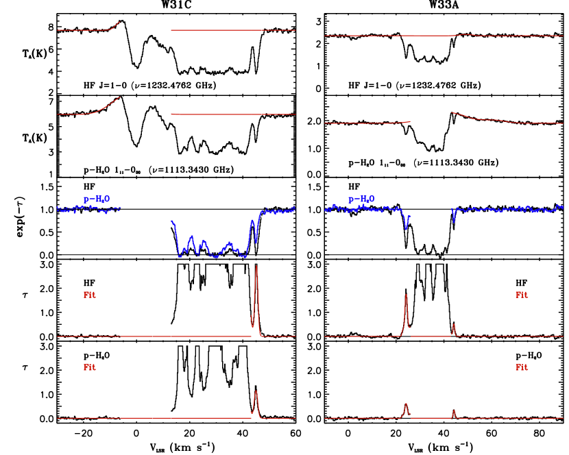
Figure 4: Same as in Figure 1 for W31C (left) and W33A (right).

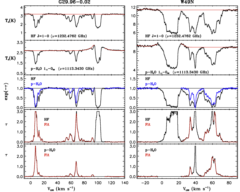
Figure 5: Same as in Figure 1 for G29.96$-$0.02 (left) and W49N (right).

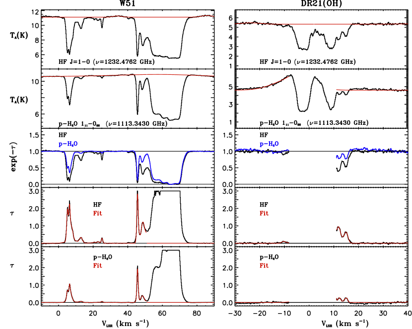
Figure 6: Same as in Figure 1 for W51 (left) and DR21(OH) (right).

3.2 Column Density Measurements

The HF and p-H₂O transitions probed here have spontaneous radiative decay rates of 2.41$\times$10^-2 s^-1 and 1.84$\times$10^-2 s^-1, respectively. These large rates require high gas densities in order for the collisional de-excitation rate to equal the spontaneous radiative decay rate for both species. The foreground gas we detect through the HF and p-H₂O absorptions arises from the Galactic diffuse ISM where gas densities have been measured to be at most $\sim$1000 cm^-3 (e.g., Jenkins & Tripp 2001; Sonnentrucker et al. 2007). In the absence of a significant sub-mm radiation field, we expect that these two species will be entirely in their ground rotational states in those foreground gas clouds (e.g., Flagey et al. 2013; Emprechtinger et al. 2013). As a result, the optical depth integrated over velocity for a gas component detected in absorption via the ground state of HF can be written as (see Neufeld et al. 2010)

$$\int{\tau dv}=4.16\times 10^{-13}N{\rm(HF/cm^{2})}\,{\rm km\,s}^{-1}.$$

Similarly, the optical depth integrated over velocity for a gas component detected in absorption via the ground state of p-H₂O is given by:

$$\int{\tau dv}=4.30\times 10^{-13}N{\rm(p-H_{2}O/cm^{2})}\,{\rm km\,s}^{-1}.$$

We used a linear combination of Gaussian components to fit the HF optical depth profiles over the LSR velocity ranges where the profiles showed optically thin or moderately thick HF absorption depths. For frequencies where the optical depth is large (the absorption lines are optically thick), noise fluctuations and small variations in the sideband gain ratio result in large uncertainties of the exact values of the optical depth in each frequency bin. We place a conservative limit of $\tau=$ 3 where (2 T_A/T_A(cont) - 1) $\leq$ 0.05. For each sight line, the gas distribution was modeled by a linear combination of Gaussian components. The initial number of Gaussian components was determined by eye and compared to the observed spectrum using a $\chi^{2}$-minimization technique. After each run, one additional Gaussian component was added to the previous model until no significant improvement to the $\chi^{2}$ value was returned by the minimization algorithm. Given the overall similarity in component distribution between HF and p-H₂O, we adopted the best-fit model of the HF spectrum (FWHM and velocity range) as our initial guess to model the p-H₂O optical depth profiles for each sight line. We followed the same optimization procedure as for HF to derive our best fit model for the H₂O spectra. We found that for one-half of our sight lines, the number of Gaussian components required to best fit the HF and p-H₂O optical depth profiles was identical. The bottom two panels of Figs. 1-6 display the HF and p-H₂O optical depth profiles (black lines). For clarity, we do not display the portion of each spectrum where blending between foreground absorption and background emission occurs. Our best fit models are over plotted as red lines only for those absorption components that are optically thin or moderately thick.

While the majority of optically thin or moderately thick absorption features from HF and p-H₂O are fitted with a single Gaussian component, some features in our sample require the use of a combination of Gaussian components. In the latter case, we sum the column densities of the individual components constituting the blended complex and report the summed column density over the gas cloud complex. To reflect these differences in sight line structures, Table 3 reports the LSR velocity range over which the optical depth absorptions were integrated rather than the individual Gaussian parameters resulting from modeling the sight lines. We only report and discuss measurements for those gas components that exhibit optically thin or moderately thick profiles ($\tau<$ 3) for both HF and H₂O.

4 Results

The spectra displayed in Figs. 1-6 show that HF is detected in all gas clouds already known to trace the diffuse ISM based on HI 21 cm observations (e.g., Lang et al. 2010), or on HCO⁺ absorption surveys (e.g., Godard et al. 2010). Our survey hence demonstrates that the diffuse molecular phase as traced by HF is as ubiquitous as the diffuse atomic phase in the Galactic spiral arms. Our survey also clearly establishes that water is as widespread as HF or H₂ in this phase. Toward the Galactic disk sources, we find that the water velocity distribution resulting from our sight line modeling is identical to that of HF, within 1 km s^-1, clearly indicating that the water distribution traces that of HF almost perfectly once $N$(H₂O) is in excess of 10¹² cm^-2. This striking similarity was noted in earlier work (Neufeld et al. 2010; Sonnentrucker et al. 2010) and is now confirmed throughout the Galactic volume we probed. One exception is the gas localized in the immediate vicinity of the Galactic Center where the HF distribution is observed to be confined to more discrete gas features than the water distribution (e.g., Lis et al. 2010; Monje et al. 2011, Sonnentrucker et al. 2013). For the Galactic disk sources in common between Flagey et al. (2013) and this paper, the velocity coincidence of the water absorption features with the extent of the continuum emission due to material close to the source led Flagey et al. (2013) to point out that the water absorption features detected toward these sources might not necessarily originate in Galactic disk gas. When combining the remarkable similarities in the HF and water distributions with the lack of evidence for significant HF emission arising from gas local to the background sources, our analysis indicates that the HF and water features we considered are mostly tracing the foreground Galactic disk material. Our conclusions are consistent with those derived in a recent Galactic [CII] survey by Gerin et al. (2015) who showed that the C⁺ absorption behaves like a foreground screen to the background sub-mm continuum sources.

Table 3 summarizes our line of sight modeling results and reports on our column density measurements as follows. Column 1 lists the LSR velocity range over which the optical depth profiles for HF and p-H₂O were integrated. Columns 2 and 3 report our column density measurements for HF, $N$(HF), and para-water, $N$(p-H₂O) with corresponding 1$\sigma$ uncertainties in units of 10¹² cm^-2. In Column 4 we list the total column density of water, $N$(H₂O)_tot, using an ortho-to-para ratio of 3 for water as measured by Flagey et al. (2013) for the Galactic disk. We note that Lis et al. (2010, 2013) measured an ortho-to-para ratio around 2.35 for water toward the Galactic Center source Sgr B2(M). This is the only value below the LTE limit that has been found so far and the effect on the H₂O column density is rather minor ($\sim$20% decrease). Finally, Column 5 reports the abundance of H₂O relative to HF, $N$(H₂O)_tot/$N$(HF) and associated 1$\sigma$ uncertainty.

We report column density measurements for both HF and p-H₂O for a total of 47 absorption features, all sight lines considered, and limits on either the p-H₂O or the HF column densities for 5 gas components. Thirty of these 47 gas features are satisfactorily modeled with a single Gaussian component within our resolution (0.3 km s^-1 at the HF frequency) and exhibit FWHM ranging from $\sim$1.0 to 4.3 km s^-1. The remaining 17 absorption complexes have ”effective” FWHM varying from $\sim$4.5 to 10 km s^-1. We also find that the FWHM derived from the p-H₂O profile modeling are identical to those for HF within 1 km s^-1, a similarity already noticed in previous work (Neufeld et al. 2010; Sonnentrucker et al. 2010) and readily seen in Figs. 1-6 in this work. Note that this similarity between the HF and H₂O distributions is genuine throughout the Galactic disk and does not result from our line of sight modeling strategy since HF and H₂O are fitted separately. Our survey therefore shows that HF and H₂O trace, in general, the same gas volumes throughout the Galactic disk. In the absence of H₂ or CH data, one can thus consider using HF to trace H₂ in gas components exhibiting H₂O absorption, as will be discussed in the next sections.

Figure 7: Distribution of the H₂O abundance relative to HF in the Galactic disk gas that we sampled. The black-contour histogram displays the distribution using all 47 measurements. The mean and median of this distribution are given in the top right corner. Four ratios differ from the mean by more than a factor of 2. When excluding those outliers (gray-shaded histogram), the distribution of the H₂O abundance relative to HF yields the mean and median values reported in the middle right.

Figure 7 displays the histogram distribution of the $N$(H₂O)/$N$(HF) ratio for the 47 features that yielded column density measurements for both HF and H₂O. With this sample, we derive a mean water abundance relative to HF of 1.73 with a standard deviation around the mean of 0.87. Four velocity ranges exhibit ratios that differ from the mean value by more than a factor of 2. When excluding the latter outliers from the distribution (gray-shaded histogram), we derive a mean H₂O to HF abundance ratio of 1.63 with a standard deviation around the mean of 0.58. The small differences in the mean values for both distributions (less than 12%) indicate that the water abundance distribution relative to HF is remarkably narrow throughout the Galactic disk and quite constant to within a factor of 2. Considering the non-Gaussian nature of the distribution, we adopted the median value of the full (47-point) distribution as our best measurement of the water abundance relative to HF, $N$(H₂O)/$N$(HF)$=$1.51, for the Galactic disk. The relative constancy of the latter ratio (to within a factor 2.5) was noted earlier by Flagey et al. (2013) for a smaller number of gas features. Their measured water abundance relative to H₂ of 5$\times$10^-8 leads to an estimate of the H₂O/HF ratio of $\sim$1.4, in agreement with our measurements within uncertainties. Our survey therefore extends the conclusions of Flagey et al. to a larger volume in the Galactic disk. We note that Flagey et al. (2013) used HF/H₂$=$3.6$\times$10^-8 which will tend to underestimate the H₂ column density and overestimate H₂O abundance relative to H₂. We also note that the deviations around the median value for the H₂O-to-HF ratio indicate that true variations in the H₂O/HF ratio do exist. In the following sections, we will argue that these variations are mostly due to local variations in the H₂O/H₂ ratio rather than variations in the HF/H₂ ratio in the ISM. As a result, our measurements offer a unique opportunity to test the physical processes as well as the chemical pathways involved in the production of gas-phase H₂O in the diffuse interstellar medium.

5 HF Abundance in the Galactic disk

In the diffuse ISM, the defining tracers of the atomic and molecular phases are atomic hydrogen (H⁰) and molecular hydrogen (H₂). Direct measurement of H₂ are most easily obtained through its ground electronic transitions which lie in the far-UV shortward of 1150Å in the Galaxy. As a result, significant effort has been dedicated for decades to identifying surrogate tracers of H₂ in the various phases of the ISM. For diffuse molecular cloud environments, combinations of FUV and optical observations have demonstrated that CH is a valuable tracer of H₂. The observed CH-H₂ relationship is routinely used to estimate H₂ column densities in the absence of H₂ observations. This relationship, however, exhibits a large but real dispersion of 0.2 dex around its mean value of 3.5$\times$10^-8 (Sheffer et al. 2008, and references therein; Levrier et al. 2012). The H₂ column densities derived from CH measurements are, thus, only accurate to within a factor of $\sim$2. The range in H₂ column densities traced by CH is also limited as the weak CH absorption is typically below detection level for diffuse molecular clouds with $N$(H₂) $\leq$${\rm few}\times$ 10¹⁹ cm^-2. CH depletion onto dust grains, or “freeze-out” limits the use of CH as a probe of H₂ in denser clouds where $N$(H₂) $\geq$ 3$\times$ 10²² cm^-2 (Mattila 1986).

Theoretical models of interstellar chemistry have predicted that HF will be the dominant reservoir of gas-phase fluorine over a large range of physical conditions (Neufeld et al. 2005; Neufeld & Wolfire 2009). In particular, HF is expected to trace H₂ both in diffuse gas with molecular fractions of only a few percent ($N$(H₂) $\geq$${\rm few}\times$ 10¹⁸ cm^-2, where CH is below the current detection limit) and in dense clouds of larger molecular fractions where HF “freeze-out” is not yet significant. As a result, HF is predicted to be the most sensitive tracer of H₂ in the diffuse molecular regime probed here. One of the goals of the PRISMAS key program was to test the latter predictions and determine whether HF could be used as a surrogate tracer of H₂ in the sub-mm range where H₂ is not observable directly. In the next sections we describe the modifications applied to our diffuse cloud models and the updates made to the chemical networks used in the models. We compare the HF observations currently available against those new model predictions and we discuss our understanding of fluorine chemistry in the diffuse ISM.

5.1 Model Modifications and Predictions

We have used a modified version of the diffuse cloud models presented in Neufeld et al. (2005) and Neufeld & Wolfire (2009). The modifications include ice freeze out and grain-surface chemistry as in Hollenbach et al. (2009), the gas-phase reactions and radiation field attenuation as in Wolfire et al. (2010), and the oxygen chemistry as in Hollenbach et al. (2012). The model consists of a slab of gas of constant hydrogen nucleus density $n_{\rm H}$, and total width $A_{V,{\rm tot}}$, which is illuminated by the interstellar radiation field, $\chi$, measured in units of the Draine (1978) field. The gas temperature and the abundances of atomic and molecular species are calculated as a function of $A_{V}$ through the cloud under the assumptions of thermal balance, and chemical equilibrium. We assume the slab is embedded in an isotropic interstellar radiation field of value $\chi$ in free-space and thus $\chi/2$ is incident on opposite sides of the slab. We use the single ray approximation given in Wolfire et al. (2010) for attenuation of the isotropic field.

An important update from the Neufeld & Wolfire (2009) paper is a new measurement for the rate of the reaction

$${\rm F}\,+\,{\rm H_{2}}\rightarrow{\rm HF}\,+\,{\rm H}$$

(Tizniti et al., 2014). This reaction is the dominant formation route for HF in regions with both high or low molecular fraction. The previously used rate was based on a fit to the calculations of Zhu et al. (2002) for an assumed ${\rm H_{2}}$ population in local thermodynamic equilibrium (LTE). The new rate is based on experimental measurements between 11 K and 295 K using a supersonic flow technique. Tizniti et al. (2014) provide a fit to the rate coefficient versus temperature assuming ${\rm H_{2}}$ in LTE. Figure 8 compares the new and old rate using the fitted functions. Over temperatures expected in diffuse gas $T\sim 50-100$ K, the new rate is a factor of $\sim 2.5$ times lower than the old rate and thus at low ${\rm H_{2}}$ abundance, the new rate results in a lower HF abundance by a factor of $\sim 2.5$. The HF abundance increases with ${\rm H_{2}}$ abundance until all of the gas phase F is locked in HF, at which point the HF abundance is insensitive to the ${\rm H_{2}\,+\,F}$ reaction rate.

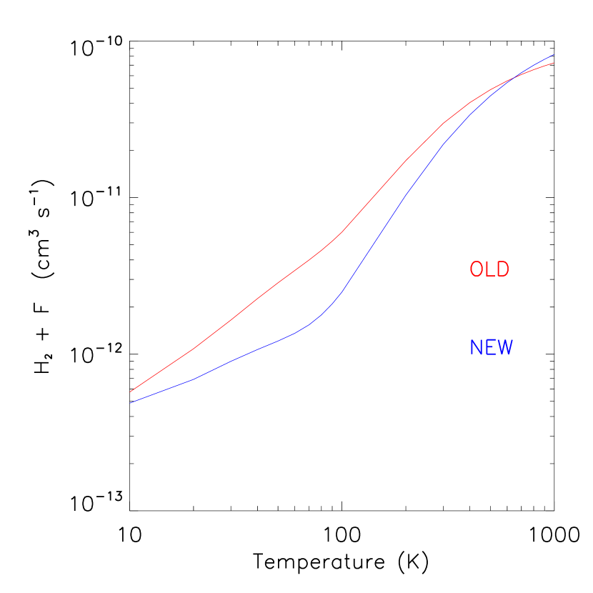
Figure 8: Reaction rates for HF production using the fitted functions given in Neufeld et al. (2005) (old rate) and Tizniti et al. (2014) (new rate). Both assume ${\rm H_{2}}$ in LTE. Over typical cloud temperatures in the diffuse ISM, the Tizniti et al. (2014) rate is a factor $\sim 2.5$ lower than the previous rate resulting in lower HF abundances.

Additional updates to the previous codes include fine-structure collision rates for O I and C I with H⁰ from Abrahamsson et al. (2007), and revised photo rates with PAHs using the Draine (1978) radiation field with linear yield functions for the ionization of PAH⁰ and electron detachment of PAH^-. Finally, an important parameter for the gas-phase production of water is the cosmic-ray ionization rate, $\zeta$. We use the definition that $\zeta$ is the primary rate per hydrogen nucleus. The ionization rate is often quoted as the total rate per ${\rm H_{2}}$ which is a factor $\sim 2.3$ times larger in molecular gas.

We have run a series of models varying the total extinction through the cloud $A_{V,{\rm tot}}$, the density $n_{\rm H}$, the cosmic-ray ionization rate $\zeta$, and the incident radiation field $\chi$. The parameters are intended to cover a range of values expected in diffuse molecular clouds (e.g., Sonnentrucker et al., 2007; Phillips et al., 2013; Goldsmith, 2013; Indriolo et al., 2013). The cloud extinction varies between $A_{V,{\rm tot}}\sim 0.05$ mag (depending on other parameters) and $A_{V,{\rm tot}}=4$ mag. The density varies between $n_{\rm H}=50$ ${\rm cm^{-3}}$ and $n_{\rm H}=900$ ${\rm cm^{-3}}$. As a standard model we use a radiation field of $\chi=1$, but examine the case $\chi=3$ as expected for the field in the inner Galaxy (Wolfire et al., 2003). We adopt a standard cosmic-ray ionization rate of $\zeta=2\times 10^{-16}$ s^-1. This rate is close to the average rate of $\sim 1.5\times 10^{-16}$ ${\rm s^{-1}}$ estimated from ${\rm H_{3}^{+}}$ column density measurements over 50 lines-of-sight by Indriolo & McCall (2012b). It is also close to the rate of $\sim 2.1\times 10^{-16}$ ${\rm s^{-1}}$ estimated by Indriolo et al. (2012a) in the sight line towards W51. Previous diffuse ISM studies adopted cosmic ray ionization rates which are lower than the standard value we adopted by a factor of $\sim$10. We investigate the effects of lower rates on our predictions as well. For the gas-phase abundances of carbon and oxygen we adopt the values of 1.6$\times 10^{-4}$ (Sofia et al., 2004) and 3.9$\times 10^{-4}$ (Cartledge et al., 2004), respectively. For fluorine, we use a gas-phase abundance value of 1.8$\times 10^{-8}$ from Neufeld et al. (2005) which amounts to $\sim 60$% of the solar abundance with the remainder depleted onto grains. Our results for the HF abundance will scale linearly with the adopted gas-phase abundance of fluorine.

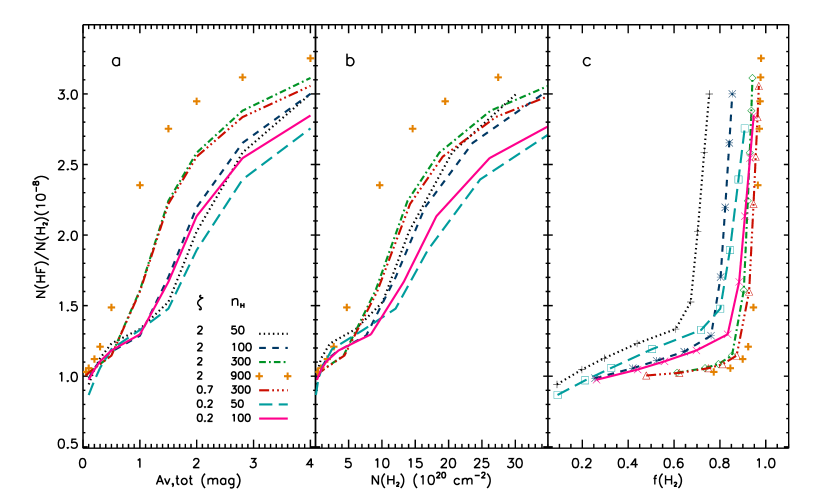
Figure 9: Predictions for the HF abundance relative to H₂ in a single cloud as a function of total visual extinction ($A_{V,{\rm tot}}$, panel a), total H₂ column density ($N$(H₂), panel b), and molecular fraction ($f({\rm H_{2}})$, panel c) using our modified 2-sided PDR model. The UV field is given in units of the Draine (1978) field, is fixed to $\chi=$1 and is assumed to be incident isotropically at a value of $\chi=$ 1/2 on each side of the cloud. In panel a), we list the range in cosmic-ray ionization rate $\zeta$ (10^-16 s^-1) and density $n_{\rm H}$ (${\rm cm^{-3}}$) we explored. In panel c), colored symbols show model predictions for clouds with $A_{V,{\rm tot}}=$ 0.1, 0.2, 0.3, 0.5, 1.0, 1.5, 2.0, 2.8 and 4.0 mag. For models ($n_{\rm H}=$ 300 ${\rm cm^{-3}}$ and $\zeta=$ 0.7$\times$10^-16 s^-1) or ($n_{\rm H}=$ 900 ${\rm cm^{-3}}$ and $\zeta=$ 2$\times$10^-16 s^-1), $A_{V,{\rm tot}}=$ 0.05 mag is also shown. To convert $A_{V,{\rm tot}}$ to hydrogen nuclei column density $N_{\rm H}=$ $N$(H⁰) + 2$N$(H₂) we use $N_{\rm H}$(cm^-2)$=$ 2$\times$10²¹ $A_{V,{\rm tot}}$.

Figure 9 shows our model predictions for the HF column density relative to the H₂ column density as a function of total visual extinction in the cloud $A_{V,{\rm tot}}$ (panel a), as a function of the total ${\rm H_{2}}$ column in the cloud $N({\rm H_{2}})$ (panel b), and as a function of the ${\rm H_{2}}$ fraction in the cloud $f({\rm H_{2}})=2N({\rm H_{2}})/[N({\rm H^{0}})+2N({\rm H_{2}})]$ (panel c). For the models shown in Fig 9, $\chi$ is fixed at $\chi=$1 in units of the Draine (1978) field. The $N({\rm HF})/N({\rm H_{2}})$ ratio is predicted to rise monotonically with increasing $A_{V,{\rm tot}}$, $N({\rm H_{2})}$, and $f({\rm H_{2}})$ and varies by at most a factor of $\sim 3$ while $\zeta$ and $n_{\rm H}$ vary by at least a factor of 10 over the entire parameter range considered here.

The dependence of the $N$(HF)/$N$(H₂) ratio on total cloud extinction $A_{V,{\rm tot}}$ can be understood by considering the dominant formation and destruction processes for HF at the cloud center. The detailed ${\rm HF}$ chemistry is presented in Neufeld et al. (2005) and Neufeld & Wolfire (2009). Briefly, the production of HF proceeds by the reaction of ${\rm H_{2}}$ with F, while the destruction occurs through reactions with ${\rm C^{+}}$, H₃⁺, He⁺, and Si⁺ plus photodissociation. For the low density models, ${\rm C^{+}}$ dominates the destruction of HF, to $A_{V,{\rm tot}}\sim 1.5$ mag, at which point electrons recombining with ${\rm C^{+}}$ lead to a lower ${\rm C^{+}}$ abundance and higher HF abundance. At high density ($n_{\rm H}\geq 300$ ${\rm cm^{-3}}$), the recombination of ${\rm C^{+}}$ is drawn to the cloud surface leading to higher HF columns even for clouds of low $A_{V,{\rm tot}}$. Increasing cloud column densities results in a drop in the C⁺ abundance and reactions with less abundant ions dominate the destruction of HF. Thus the HF destruction rates fall and the $N$(HF)/$N$(H₂) ratio rises.

Since both the HF column density and ${\rm H_{2}}$ column density depend on the ${\rm H_{2}}$ abundance, the ratio does not depend directly on the ${\rm H_{2}}$ abundance. In addition, since both the formation of HF and destruction of HF have the same dependence on density ($\propto n^{2}$), the HF fractional abundance is not directly density dependent. As a result, we only see a weak density dependence in Figure 9.

The HF abundance predictions are also mostly insensitive to variations in $\zeta$. Note that a slight increase of the HF abundance of at most 10% is predicted at $A_{V,{\rm tot}}$= 4 mag for $n_{\rm H}$ $\leq$ 100 cm^-3 when increasing $\zeta$ by a factor of 10. Cosmic rays play a role in the destruction of both HF and H₂, as they produce H₃⁺ and He⁺ which then react with HF and H₂. The decrease in the H₂ abundance is greater than that in the HF abundance which, in turn, results in the $\sim$10% increase in the $N$(HF)/$N$(H₂) ratio seen in Fig. 9.

5.2 HF Observations

The grid of model calculations presented in the previous section predicts that the column density of HF with respect to H₂ varies between $N({\rm HF})/N({\rm H_{2}})$ $\sim$ 0.9 $\times 10^{-8}$ at the cloud surface ($A_{V,{\rm tot}}\sim$ 0.08 mag) in the low density regime to $N({\rm HF})/N({\rm H_{2}})\sim 3.3\times 10^{-8}$ at the cloud center ($A_{V,{\rm tot}}\sim$ 4 mag) in the high density regime considered here. As a result, HF is predicted to be a very sensitive probe of H₂, as it can trace H₂ both in mostly diffuse atomic gas ($f$(H₂)$\leq$ 0.1) and in mostly diffuse molecular gas (0.1$<$ $f$(H₂) $\leq$0.9) in the interstellar medium. The HF abundance in our models never reaches the value of 3.6 $\times$ 10^-8 expected if all gas-phase F is locked into gas-phase HF; a value derived from FUV measurements of the abundance of gas-phase atomic fluorine (e.g., Snow et al. 2007). The leveling off around a value of 3.3 $\times 10^{-8}$ seen in Fig. 9 for $n_{\rm H}$ = 900 cm^-3, is due to the incomplete conversion of F into HF in the outer regions of the cloud. If the gas becomes fully molecular slightly before all F is locked in HF, then the total column density ratio $N$(HF)/$N$(H₂) is less than the F abundance.

Following the first Herschel/HIFI detections of the ground rotational transition of HF toward sight lines comprised mostly of diffuse atomic/molecular clouds (Neufeld et al. 2010; Sonnentrucker et al. 2010), numerous additional HF detections were reported both with the high resolution HIFI data and the lower resolution SPIRE and PACS data (e.g., Kirk et al. 2010). At this point in time, HF has been detected in the Galactic Center (e.g., Sonnentrucker et al. 2013; Goicoechea et al. 2013), in hot cores around massive proto-stars (e.g., Phillips et al. 2010; Emprechtinger et al. 2012), in the ISM of extra-galactic sources up to z=2.6 (e.g., Monje et al. 2011; Monje et al. 2014) and in the Galactic disk (Flagey et al. 2013; this work). These studies clearly established the ubiquitous presence of the HF molecule in the interstellar medium, as predicted by our models and as expected from a tracer of H₂.

The $N$(HF)/$N$(H₂) values currently available in the literature range from 1.0 $\times$ 10^-8 to 2.5$\times$ 10^-8 (e.g. Sonnentrucker et al. 2010; Phillips et al. 2010, Monje et al. 2011; Emprechtinger et al. 2012) and are fully consistent with our model predictions. With the exception of the HF/H₂ ratio estimated by Indriolo et al. (2013) and discussed below, those ratios were estimated indirectly from simultaneous measurements of HF and either CH or ¹³CO along these sight lines. The CH column densities were converted into H₂ columns using the most recent estimate of the CH-H₂ relationship $N$(CH)/$N$(H₂)=3.6 $\times$ 10^-8 (Sheffer et al. 2008). As mentioned earlier, the CH-H₂ relationship exhibits a standard deviation of about 0.2 dex that is real and thought to be related to the chemical pathways involved in the formation of CH in the diffuse ISM. The ¹³CO column densities where converted to H₂ columns for a given carbon Galactic isotopic ratio and for a given CO-to-H₂ ratio; the latter two quantities also vary by factors of a few in the Galactic disk (Sonnentrucker et al. 2007; Langer & Penzias 1990). With these caveats in mind, it is interesting to note that the range in the $N$(HF)/$N$(H₂) ratio measured to-date with Herschel is fully consistent with our model calculations, thus, validating our understanding of both the physical conditions and the new reaction rates involved in the chemistry of interstellar fluorine.

A few direct measurements of $N$(HF)/$N$(H₂) were recently obtained by Indriolo et al. (2013) for a handful of targets sampling diffuse molecular clouds where $N$(H₂) and $N$(HF) were derived from FUV and near-IR observations, respectively. For all sight lines where measurements of both quantities were obtained, Indriolo et al. (2013) derived $N$(HF)/$N$(H₂) ratios between 0.5 and 1.4 $\times$ 10^-8. Of particular interest are the results obtained toward the translucent sight line HD154368. This sight line was best modeled to be comprised of diffuse molecular material with $n_{\rm H}$= 325 cm^-3, $\chi$=3 and $\zeta$= 0.5$\times$ 10^-16 s^-1 by Spaans et al. (1998) while FUV measurements based on C₂ observations yielded $n_{\rm H}$= 240 cm^-3 (Sonnentrucker et al. 2007). Our model calculations for the HF abundance using the parameters from Spaans et al. (1998) and an average density of $n_{\rm H}$ = 300 cm^-3 yield a ratio of $N$(HF)/$N$(H₂) = 2.14 $\times$ 10^-8 toward this sight line. Our model predictions are consistent with the direct measurements of Indriolo et al. (2013) of $N$(HF)/$N$(H₂) = 1.15 $\pm$ 0.41 within 3-$\sigma$. In summary, all measurements obtained to date -whether direct or indirect- corroborate the prediction that HF can be used as a surrogate tracer of H₂ in the diffuse ISM, down to very low molecular fractions where CH is typically below our detection level. Since direct H₂ measurements are not available for the entire set of HF and H₂O absorption features we report in this survey, we will use the HF column densities we derive as proxies for H₂ in the remainder of the paper.

6 H₂O Abundance in the Galactic disk

6.1 Model Predictions

Figure 10 shows the predictions of the PDR model described in the previous section for the ${\rm H_{2}O}$ column density relative to the H₂ column density as a function of total visual extinction in the cloud ($A_{V,{\rm tot}}$, panel a), as a function of the total ${\rm H_{2}}$ column density in the cloud ($N({\rm H_{2}})$, panel b) and as a function of the molecular fraction in the cloud ($f({\rm H_{2}})$, panel c). The UV field is given in units of the Draine (1978) field and is fixed to $\chi$=1.

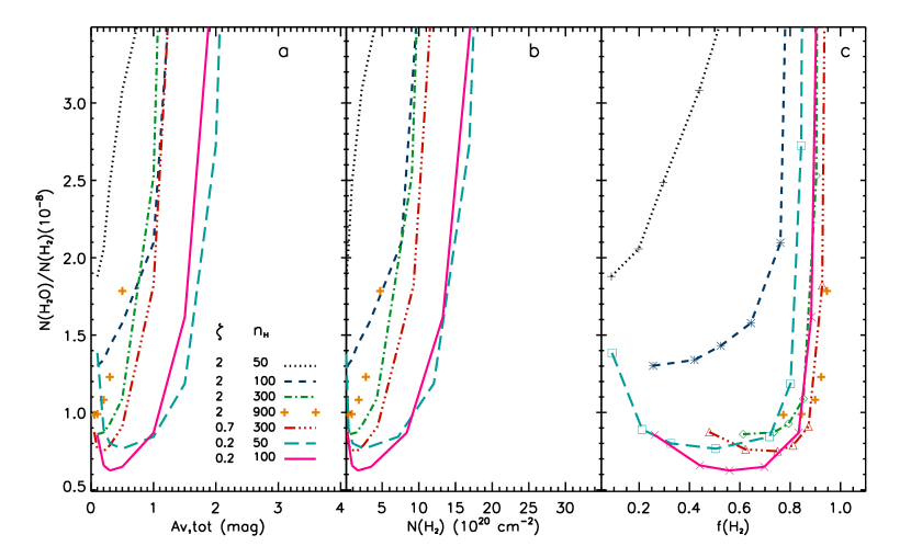
Figure 10: Predictions for the H₂O abundance relative to the H₂ in a single cloud as a function of total visual extinction ($A_{V,{\rm tot}}$, panel a), total H₂ column density ($N$(H₂), panel b), and molecular fraction ($f({\rm H_{2}})$, panel c) using our modified 2-sided PDR model. The UV field is given in units of the Draine (1978) field, is fixed to $\chi=$1 and is assumed to be incident isotropically at a value of $\chi=$ 1/2 on each side of the cloud. In panel a), we list the range in cosmic-ray ionization rate $\zeta$ (10^-16 s^-1) and density $n_{\rm H}$ (${\rm cm^{-3}}$) that we explored. In panel c), colored symbols show model predictions for clouds with $A_{V,{\rm tot}}=$ 0.1, 0.2, 0.3, 0.5, 1.0, 1.5, 2.0, 2.8 and 4.0 mag. For models ($n_{\rm H}=$ 300 ${\rm cm^{-3}}$ and $\zeta=$ 0.7$\times$10^-16 s^-1) or ($n_{\rm H}=$ 900 ${\rm cm^{-3}}$ and $\zeta=$ 2$\times$10^-16 s^-1), $A_{V,{\rm tot}}=$ 0.05 mag is also shown. To convert $A_{V,{\rm tot}}$ to hydrogen nuclei column density $N_{\rm H}=$ $N$(H⁰) + 2$N$(H₂) we use $N_{\rm H}$(cm^-2)$=$ 2$\times$10²¹ $A_{V,{\rm tot}}$.

The ${\rm H_{2}O}$ chemistry was discussed in detail by van Dishoeck & Black (1986), Hollenbach et al. (2009, 2012), and van Dishoeck et al. (2013). As in the case of HF, the variations in the H₂O abundance reflect the competition between the formation and destruction processes that contribute over the parameter range explored here. In brief, the destruction of ${\rm H_{2}O}$ is dominated by photodissociation and, at low $A_{V}$, has some contribution by reaction with ${\rm C^{+}}$. The production of ${\rm H_{2}O}$ proceeds by a combination of surface chemistry on grains and ion-neutral chemistry in the gas phase. When the molecular fraction is low the ion-neutral chemistry in the gas phase is initiated by cosmic-ray ionization of atomic H, while when the molecular fraction is high, the ion-neutral chemistry is initiated by cosmic-ray ionization of ${\rm H_{2}}$. In both the atomic and molecular branches the rate of production of ${\rm H_{2}O}$ increases with the ${\rm H_{2}}$ abundance since both branches require reactions with ${\rm H_{2}}$ to proceed in the gas phase. When both the ${\rm H_{2}}$ and electron abundances are high, the production of water can be reduced due to electron recombinations with ${\rm H_{3}^{+}}$. When the ${\rm H_{2}}$ abundance is low, but the electron abundance remains high, the water production can be reduced by electron recombination with ${\rm H^{+}}$ or by neutralization of ${\rm H^{+}}$ by ${\rm PAH^{-}}$ or by PAH. Finally, when the H₂ abundance is high, but the electron abundance is low, the gas-phase production of H₂O proceeds efficiently through ion-molecule reactions.

To further explain the physical regimes where the various processes dominate, we start with a typical diffuse cloud visual extinction ($A_{V,{\rm tot}}=$ 0.5 mag), density ($n_{\rm H}=$100 ${\rm cm^{-3}}$), and cosmic-ray ionization rate ($\zeta=$ 2$\times$10^-16 s^-1), and then discuss the variation in the H₂O production, while varying these parameters. For the $A_{V,{\rm tot}}\sim 0.5$ mag and $n_{\rm H}\leq 100$ ${\rm cm^{-3}}$ models, the production of ${\rm H_{2}O}$ is dominated by ion-neutral chemistry through the cosmic-ray ionization of atomic hydrogen. To first order the ${\rm H_{2}O}$ abundance scales as $\zeta/n_{\rm H}$ and thus increasing density results in a lower $N({\rm H_{2}O})/N({\rm H_{2}})$ ratio, for a given cosmic-ray rate.

For models $n_{\rm H}\geq 300$ ${\rm cm^{-3}}$, the molecular fraction rises and the atomic hydrogen abundance falls sufficiently so that the ion-molecule chemistry proceeds mainly through cosmic-ray ionization of ${\rm H_{2}}$. However, for these models, the electron abundance remains high and the gas-phase production of ${\rm H_{2}O}$ is reduced due to the recombination of ${\rm H_{3}^{+}}$, an intermediary in this particular H₂O production route. As a result, ${\rm H_{2}O}$ is produced mainly by reactions on grains. In the limit of ${\rm H_{2}O}$ produced by grain chemistry alone and destroyed by photodissociation, the $N({\rm H_{2}O})/N({\rm H_{2}})$ ratio is a function of $n_{\rm H}/\chi$ (Hollenbach et al., 2009).

For the $A_{V,{\rm tot}}\sim$0.5 mag, $n_{\rm H}=$300 ${\rm cm^{-3}}$, and $\zeta=$0.7$\times$10^-16 s^-1 model, only $\sim 15$% of the water is predicted to be produced through gas-phase reactions. For the lowest cosmic ray rate we tested ($\zeta=0.2\times 10^{-16}$ ${\rm s^{-1}}$), the models with $n_{\rm H}\geq 100$ ${\rm cm^{-3}}$ and $\chi=1$ are dominated by grain surface chemistry and increasing the density $n_{\rm H}$ produces more water and, hence, higher $N({\rm H_{2}O})/N({\rm H_{2}})$.

At lower $A_{V,{\rm tot}}$ ($<0.5$ mag), curves for which grain surface chemistry dominates are seen to rise. Since the grain surface chemistry reactions do not depend on the ${\rm H_{2}}$ abundance, the curves rise as the ${\rm H_{2}}$ abundance drops. At higher $A_{V,{\rm tot}}\geq$ 2 mag, for all models, the electron abundance drops sufficiently due to absorption of FUV photons, so that water can be produced efficiently by ion-molecule chemistry.

We note that Dulieu et al. (2013) have presented experimental evidence to suggest that OH and H₂O formed on bare silicate grain surfaces can be chemically desorbed upon formation. We consider the effects of chemical desorption by assuming that 30% of the OH is immediately desorbed and 70% of the H₂O is immediately desorbed (see their Fig. 4). We find at most a $\sim$ 60% increase in the H₂O column density over our model parameter space. The effect is largest where surface chemistry dominates the production of H₂O and for the smallest cloud column densities. The increase drops to $\sim$ 40% for a total cloud column density of $A_{V,{\rm tot}}$ =2.0, and drops to $\sim$ 10% for a total cloud column density of $A_{V,{\rm tot}}$ = 4.0. We also note that Minissale et al. (2013), and Minissale et al. (2014) have found that O-atom diffusion can be quite rapid on grain surfaces leading to the production of O₂ and O₃. This process is important deep in molecular clouds where the incidence of oxygen atoms exceeds that of H. These conditions are, however, not applicable to the models presented here.

6.2 H₂O Observations

Since H₂ is not observable directly in the sub-mm, efforts are made to find surrogate tracers of H₂ in this wavelength domain in order to obtain abundance measurements relevant to test our knowledge of diffuse cloud chemistry. In Section 5, we demonstrated that HF can be used as a surrogate tracer of H₂, down to much lower molecular fractions than the more typical tracers such as CH. Since we do not have H₂ or CH column density measurements for all 47 features presented here, we use HF as a tracer of H₂ and discuss the H₂O abundance relative to HF -$N$(H₂O)/$N$(HF)- in the remainder of this paper.

As described in Section 4, we detected absorption from H₂O toward all 12 sight lines included in our survey and we measured its column density in a total of 47 cloud components (see Table 3). We compared our H₂O column density measurements against those reported by Flagey et al. (2013) for the 17 gas components in common to both studies; these are detected in the foreground to W49N, W51, G34.3$+$0.1, W33A and DR21(OH). We find that the two sets of measurements are consistent within 2 $\sigma$ for 13 components. For four components, the H₂O column densities we measured are either lower by 50% (DR21(OH)) or higher by up to a factor of 3 (G34.3$+$0.1 and W49N) than those reported by Flagey et al. (2013). In all four cases, the background continua local to these gas components are somewhat affected by the presence of water emission local to the sources; the discrepancies we noted above are readily explained by the different methods we adopted to account for the background emission toward each source and give a measure of the modeling uncertainty in such cases. The H₂O column density measurements we report for these 4 velocity components (marked with an asterisk in Table 3) should be used with caution.

Flagey et al. (2013) reported no dependence of the H₂O abundance relative to H₂ on Galactocentric distance for the 6 sources they considered. For those sources located in the inner Galaxy in our extended survey, we computed a Galactocentric distance for each cloud we detected in HF and H₂O based on the source longitude and V_LSR to see whether the variations in the $N$(H₂O)/$N$(HF) we measure show a dependence on position in the Galaxy. We find no dependence of the $N$(H₂O)/$N$(HF) ratio with Galactic radius either, a conclusion consistent with that of the smaller Flagey et al. (2013) survey. Our results therefore add weight to the conclusion that the variations in the $N$(H₂O)/$N$(HF) ratio we measure can be considered representative throughout the Galactic disk. With a median value of $N$(H₂O)/$N$(HF) = 1.51 in diffuse clouds, H₂O also appears as an alternative tracer of H₂ (within a factor of 2.5) in the absence of HF or CH spectra, as already suggested in Flagey et al. (2013).

The comparison of our model predictions displayed in Fig. 9 and Fig. 10 shows that, in the diffuse molecular cloud regime ($f_{\rm H_{2}}\leq 0.5$), the column density ratio of H₂O-to-HF varies from 0.5 $\leq$ $N$(H₂O)/$N$(HF) $\leq$ 3, all models considered. Our models predict that the water abundance relative to HF varies by up to a factor 6, depending on the local gas physical conditions. The model comparisons further show that the variations in the $N({\rm H_{2}O})/N({\rm H_{2}})$ ratio are much larger (factor of 2 to 4) than the variations in the $N({\rm HF})/N({\rm H_{2}})$ ratio (at most factor of 2) both as a function of cloud column density for a given set of parameters and between models with different input parameters. Our models further predict that the variations in the $N$(H₂O)/$N$(HF) are mostly driven by variations in the H₂O column density, rather than in the HF column densities for a given set of model parameters.

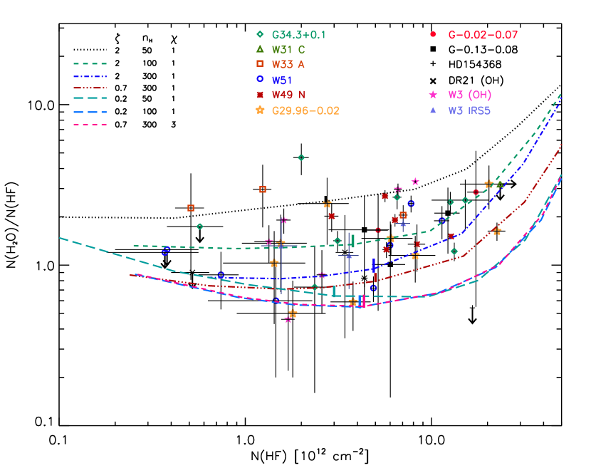
Figure 11: H₂O column density relative to that of HF versus HF column density throughout the Galactic disk probed by our Herschel survey. Each sight line is represented by a particular symbol and color which are listed at the top of this figure. Overplotted on our measurements are the predictions obtained from a series of 2-sided PDR model runs. The parameter space explored in our runs is listed in the upper left of the panel with $\zeta$ in units of 10^-16 s^-1 and $n_{\rm H}$ in units of cm^-3. 1 $\sigma$ uncertainties are over plotted for each measurement. 3-$\sigma$ uncertainties are displayed for all upper limits. The colored vertical bars over plotted on each model run correspond to a depth in the cloud of $A_{V,\rm tot}\sim 0.5$ mag. The upper limit for HD154368 was derived using H₂O results from Spaans et al. (1998) and HF and H₂ results from Indriolo et al. (2013).

In Figure 11 we display the $N$(H₂O)/$N$(HF) ratio versus $N$(HF) for all 47 foreground clouds with optically thin or moderately thick absorptions. The measurements toward each sight line are represented by a particular symbol and color that are listed at the top of the panel. We over-plot our model predictions for the $N$(H₂O)/$N$(HF) ratio onto our measurements using the same symbol and color coding as in Figs 9 &10. The range of model parameters we use is listed at the top left of the panel. We use a log-log scale for both axes for clarity purposes. 1$\sigma$ uncertainties are shown for all measurements and 3$\sigma$ uncertainties are plotted as downward arrows for upper limits in the water abundance. This figure shows that the $N$(H₂O)/$N$(HF) ratio varies by about a factor 5 overall; our observational results are therefore fully consistent with the model predictions presented here and known to best bracket the physical conditions in diffuse clouds.

Our sight line analyses (Section 2) indicated that HF and H₂O are co-located in the gas components we detect throughout the Galactic disk, meaning that both molecules are subject to the same physical conditions within each gas clump along the sight lines. As a result, the variations we measure are not caused by differences in the spatial distributions of HF or H₂O along a given sight line (geometric effects) but are caused by true variations in the molecular content for a given gas component.

In particular, Fig. 11 displays a subtle break in the water abundance relative to HF once $N$(HF)$=$5$\times$10¹² cm^-2. For $N$(HF) $\leq$ 5$\times$10¹² cm^-2, our measurements indicate that the $N$(H₂O)/$N$(HF) ratio varies by about a factor of 6 to 9 from $\sim$ 0.5 to 4.6. The lowest water abundances relative to HF are best reproduced by models with low cosmic ray ionization rates ($\zeta\leq 0.7\times$10^-16 s^-1) over the density range known to be representative of the diffuse ISM while the highest water abundances relative to HF are best represented by $\zeta\sim 2\times$10^-16 s^-1 and $n_{\rm H}\leq$ 100 cm^-3. The prevalence of mixtures of physical conditions within the galactic disk diffuse ISM and along any given sightline has long been recognized and is clearly evidenced here again, as multiple model runs can accommodate our measurements for this particular HF column density range.

For $N$(HF) $>$ 5$\times$10¹² cm^-2, however, our measurements are not consistent with models using $\zeta\leq 0.7\times$10^-16 s^-1. As a matter of fact, over 80% of our measurements in this specific HF column density range show water abundances relative to HF consistent with model predictions for single clouds with $\zeta=2\times$10^-16 s^-1, $\chi=$1 and n${}_{\rm H}\leq$100 cm^-3. The variations in the measured $N$(H₂O)/$N$(HF) in this HF regime amount to at most a factor of 3, thus, pointing toward a population of low gas density clouds with properties intrinsically very similar. Considering that the HF abundance relative to H₂ currently measured varies by at most a factor of $\sim$2 (see Section 5), we conclude that the variations we measured in the $N$(H₂O)/$N$(HF) ratio are mostly driven by variations in the H₂O/H₂ ratio within the gas clouds we probe.

7 Discussion

In the diffuse ISM, the production of H₂O within our models proceeds via both gas-phase reactions and grain-surface chemistry. Since the contribution of each mechanism depends on the cloud physical conditions, our measurements give us a unique opportunity to test the chemical pathways predicted to lead to H₂O formation in this regime.

In Figure 12, we show the fractional rate of H₂O production on grain surfaces compared to the total production rate of H₂O as a function of $N$(HF). The rates are evaluated at cloud center where the H₂O abundance is generally highest and dominates the contribution to the column density. These curves can be directly compared with those in Figure 11.

As already mentioned in Section 6, at a column of $N$(HF) $\approx$ 5$\times$10¹² cm^-2 and for $n_{\rm H}\leq$ 100 cm^-3, the production of H₂O is dominated by ion-neutral chemistry (see Fig.12). The H₂O abundance scales as $\zeta$/$n_{\rm H}$ and thus a larger density results in a lower $N$(H₂O)/$N$(HF) ratio for a given cosmic-ray rate (Fig. 11). At higher densities $n_{\rm H}>$ 300 cm^-3, grain-surface reactions dominate the production of water. Figure 12 shows that for $n_{\rm H}=$ 300 cm^-3 and $\zeta=$ 0.7$\times$10^-16 s^-1 only about 15% of the water is produced through gas-phase reactions.

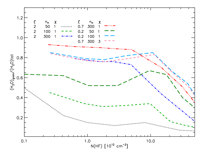
Figure 12: Fractional rate of H₂O production on grain surfaces compared to the total production rate of H₂O versus HF column density in the column density range probed by the survey. The parameter space explored in our runs is listed in the upper section of the panel with $\zeta$ in units of 10^-16 s^-1 and $n_{\rm H}$ in units of cm^-3. The UV field is given in units of the Draine (1978) field and is fixed to $\chi=$1 or $\chi=$3.

For $N({\rm HF})$ $<5\times 10^{12}$ ${\rm cm^{-2}}$ ($A_{V,\rm tot}$ $<0.5$ mag) , the curves for which grain surface chemistry dominates are seen to rise in Fig. 10. Since the grain chemistry reactions do not depend on the ${\rm H_{2}}$ abundance while the HF production does, the curves rise as the ${\rm H_{2}}$ and thus HF abundance drops. At higher $A_{V,\rm tot}$, the electron abundance drops sufficiently due to absorption of FUV photons, so that water can then be produced efficiently through the cosmic-ray ionization of ${\rm H_{2}}$. The curves thus rise due to an increasing abundance of ${\rm H_{2}O}$.

Note that in the limit in which ${\rm H_{2}O}$ is produced by grain surface chemistry alone and destroyed by photodissociation, while HF is both formed and destroyed by gas-phase reactions, the ratio $N({\rm H_{2}O})/N({\rm HF})$ is a function of $n_{\rm H}/\chi$ (see Figs. 11 & 12). For the lowest cosmic ray rate we considered here ($\zeta=0.2\times 10^{-16}$ ${\rm s^{-1}}$), the curve for $n_{\rm H}=100$ ${\rm cm^{-3}}$ and $\chi=1$ lies close to the curve for $\zeta=0.7\times 10^{-16}$ ${\rm s^{-1}}$, $n_{\rm H}=300$ ${\rm cm^{-3}}$ and $\chi=3$, as expected for ${\rm H_{2}O}$ production by grain chemistry (see Fig. 12).

Our measured water abundances relative to HF reported in Table 3 are all bracketed by model predictions based on a grid of gas physical conditions known to be representative of the diffuse ISM. At low visual extinctions and for densities greater than $n_{\rm H}=$100 cm^-3, our models predict that grain-surface chemistry is necessary to account for some of our observations. For $A_{V,\rm tot}$ $\geq$ 0.5 mag, our models indicate that contributions from both gas-phase and grain-surface chemistry are required to account for our measurements as well. The contribution of each production mechanism depends intimately on the electron density distribution within the cloud, as recombination with H⁺ and H${}_{3}^{+}$ inhibit the gas-phase production routes.

Within our uncertainties, most measurements are compatible with more than one model. These degeneracies are mainly due to two factors. Firstly, some of our model predictions are degenerate and measurements of HF and H₂O alone do not allow us to lift the model degeneracies; additional observational probes such as HCO⁺ (e.g., Godard et al. 2014) are necessary to do so. Secondly, our measurements are not obtained toward true single clouds contrary to the model assumptions, as discussed earlier. To compare the water abundance relative to HF versus HF column density on equal footing one would have to determine the HF column density in each gas clump along a given sight line, a task which is observationally very challenging. One rare exception might be the sight line toward HD154368. As mentioned earlier, Spaans et al. (1998) and Rachford et al. (2002) determined that true translucent conditions are present in the gas intercepting the sight line to this star. The decomposition performed by Rachford et al. (2002) suggests that $\sim$73% of the H₂ gas observed with FUSE data belongs to the translucent phase. As a result, it is reasonable to assume that $\sim$73% of the total HF column density we measure is also associated with this translucent phase. Correcting the total measured HF column density by that fraction has the effect of moving the upper limit on the $N$(H₂O)/$N$(HF) ratio to the left (or $N$(HF)$\sim$ 1.2 $\times$10¹³ cm^-2) in the bottom panel of Fig. 11. One can see that the overall impact of such a sight line “decomposition” on our measurements would primarily be to shift the distribution horizontally and to the left - or to lower $N$(HF).

Despite these degeneracies, it is important to note that the lower envelope on the $N$(H₂O)/$N$(HF) ratios we measure is too high to understand without grain-surface chemistry being important. The overall range in $N$(H₂O)/$N$(HF) ratios that we observe in itself demonstrates the importance of grain surface chemistry in the production of water in this diffuse ISM. It is also remarkable to see that the adopted physical conditions and chemical network that best bracket our observations remain largely unaltered, when taking the latter distribution shift into account. Our measurements therefore indicate that the range in densities, FUV and cosmic-ray ionization rates required to model our observations are not only pervasive throughout the diffuse gas composing the Galactic disk but they are also quite tightly constrained. Finally, our results also validate our understanding of the various chemical pathways thought to lead to the gas-phase abundance of HF and H₂O in the diffuse ISM. While most chemical pathways involve gas phase reactions in diffuse clouds, our measurements do confirm that grain surface chemistry also plays a significant role in the production of gas-phase water in such low density environments.

We note that the effects of turbulent dissipation regions (TDR) on the chemistry in diffuse clouds were recently extensively tested and were found to successfully reproduce the wealth of CH⁺ and SH⁺ absorption measurements obtained with Herschel toward sight lines probing the diffuse ISM (Godard et al. 2014 and references therein). The production of gas-phase water was also included in those models. Godard et al. (2014) found that for gas densities in the range we probe here ($n_{\rm H}$= 50-300 cm^-3) and for $A_{V,\rm tot}$$\sim$0.5 mag and a primary cosmic ray rate per H of 0.4$\times$10^-16 s^-1 cm^-3, TDR could contribute up to 50% of the total (TDR plus ion-molecule) gas-phase production of water. The Godard et al. (2014) models do not include the effect of grain-surface chemistry, while our models do not include the effects of TDR on the water production, hence a direct comparison of these model predictions is not feasible. However, all differences considered and for this particular set of parameters, our models predict that grain surface chemistry produces up to 85% of the observed gas-phase water abundance, with ion-molecule reactions producing 15% of the observed gas-phase water abundance. Consequently, ion-molecule reactions combined with TDR effects alone (without any contribution from grain surface chemistry) would fall short ($\sim$35% of that required) in terms of reproducing the observed water abundance measured in this survey.

8 Conclusions

We have presented the most comprehensive survey of HF and H₂O observations obtained in the diffuse interstellar medium of the Galactic disk using the Herschel/HIFI instrument. The column density of both molecules is measured toward 47 discrete gas components detected in absorption and probing the Galactic disk volume. We demonstrate that both molecules are ubiquitous in the diffuse gas of our Galaxy. We find that the HF and H₂O velocity distributions trace each other almost perfectly, in the disk, establishing that HF and H₂O essentially probe the same gas-phase volume.

We compare our observations to state-of-the-art diffuse cloud models that were modified to include grain surface chemistry, as well as updated reaction rates for the fluorine chemistry. Our measurements corroborate theoretical predictions that HF is a very sensitive tracer of H₂ down to molecular fractions of a few percent, a regime where more common tracers such as CH are below detection level.

We have used HF as a surrogate tracer of H₂ to study the variation of the H₂O column density -relative to HF- within the Galactic disk diffuse gas. We find that the $N$(H₂O)/$N$(HF) ratio shows a narrow distribution with a median water abundance relative to HF of 1.51. Our results therefore add weight to the previous suggestion that H₂O can also be used as tracer of H₂- within a factor of 2.5- in the diffuse ISM, in the absence of HF or CH observations.

We have demonstrated that the overall variations of a factor of 2.5 around the median in the $N$(H₂O)/$N$(HF) ratio are driven by true variations in the H₂O column density within the disk. Our measurements, therefore, provide us with a unique opportunity to test the chemical pathways predicted to play a role in the water production in the diffuse ISM. We find that the range in water abundances relative to HF that we measure could only be explained if significant grain surface chemistry production occurred in addition to gas-phase ion-molecule production. While most chemical pathways involve gas phase reactions alone in the diffuse ISM, our survey confirms that grain surface chemistry can play a significant role in the production of some molecular species, such as gas phase H₂O, in this low density environment.

Table 1: Target List.

Target	RA	Dec	$l$	$b$	$D$	Ref.
	(h) (m) (s)	(∘) (′)(′′)	(∘)	(∘)	(kpc)
W3 IRS5	02  25  40.6	$+$62  05  51.0	133.715	$+$1.215	1.83	1
W3(OH)	02  27  03.8	$+$61  52  25.0	133.946	$+$1.06	2.04	2
G$-$0.02$-$0.07	17  45  50.2	$-$28  59  53.0	359.97	$-$0.07	8.34	3
G$-$0.13$-$0.08	17  45  37.4	$-$29  05  40.0	359.30	$-$0.432	8.34	3
G34.3+0.1	18  53  18.7	$+$01  14  58.0	34.26	$+$0.15	3.80	4
W28A	18  00  30.4	$-$24  04  00.0	5.9	$-$0.39	1.28	5
W31C	18  10  28.7	$-$19  55  50.0	10.62	$-$0.38	4.95	6
W33A	18  14  39.4	$-$17  52  00.0	12.91	$-$0.26	2.40	7
G29.96$-$0.02	18  46  03.9	$-$02  39  21.9	29.96	$-$0.02	5.26	8
W49N	19  10  13.2	$+$09  06  12.0	43.17	$+$0.01	11.1	9
W51	19  23  43.9	$+$14  30  31.0	49.49	$-$0.39	5.41	10
DR21(OH)	20  39  01.0	$+$42  22  48.0	81.72	$+$0.57	1.50	11

References: 1- Imai et al. (2000); 2- Hachisuka et al. (2006) ; 3- Reid et al. (2014); 4- Fish et al. (2003); 5- Motogi et al. (2011); 6- Sanna et al. (2014); 7- Immer et al. (2013); 8- Zhang et al. (2014); 9- Zhang et al. (2013) ; 10- Sato et al. (2010); 11- Rygl et al. (2012)

Table 2: Observation Summary.

Target	texp(HF)	TA(cont)[HF]a	texp(H2O)	TA(cont)[H2O]a	Observation Dates	HF & H2O Obs IDs
	(s)	(K)	(s)	(K)		starting with 1342:
W3 IRS5	492	3.56 $\pm$ 0.10	2965	3.11 $\pm$ 0.02	2012-07-20 & 2010-07-18	248382-83-84 & 201591
W3(OH)	9275	4.46 $\pm$ 0.03	3540	4.14 $\pm$ 0.03	2013-03-27 & 28	268474-75-76 & 268605-06-07
G$-$0.02$-$0.07	3693	0.93 $\pm$ 0.04	2139	0.92 $\pm$ 0.04	2010-10-06	205885-86-87 & 205882-83-84
G$-$0.13$-$0.08	746	1.43 $\pm$ 0.11	428	1.39 $\pm$ 0.11	2011-09-14	228613-14 & 228615-16
G34.3+0.1	522	9.20 $\pm$ 0.12	246	7.57 $\pm$ 0.10	2010-04-18	195074-75-76 & 195070-71-72
W28A	562	6.03 $\pm$ 0.10	426	4.71 $\pm$ 0.06	2011-03-11	215860-61-62 & 215863-64-65
W31C	534	7.74 $\pm$ 0.11	306	5.99 $\pm$ 0.09	2010-03-05	191690-91-92 & 191687-88-89
W33A	3775	2.36 $\pm$ 0.04	2694	1.91 $\pm$ 0.03	2011-03-11	215875-76-77 & 215872-73-74
G29.96$-$0.02	9162	3.20 $\pm$ 0.03	2824	2.69 $\pm$ 0.01	2013-03-27 & 2011-09-29	268483-84-85 & 229875-76
W49N	522	11.48 $\pm$ 0.18	246	9.06 $\pm$ 0.16	2010-03-22	192595-96-97 & 192592-93-94
W51	9259	11.12 $\pm$ 0.04	3582	10.51 $\pm$ 0.04	2013-03-27 & 28	268478-79-80 & 268611-12-13
DR21(OH)	1014	5.36 $\pm$ 0.06	1086	4.56 $\pm$ 0.05	2010-05-12	196502-03-04 &196506-07-08

Table 3: Column Density Measurements.

$V_{\rm LSR}$ Range	$N$(HF)	$N$(p-H2O)	$N$(H2O)tot	$\frac{N({\rm H_{2}O})_{\rm tot}}{N({\rm HF})}$
(km s-1)	(1012 cm-2)	(1012 cm-2)	(1012 cm-2)
W49N
$+$30,$+$34*	12.74$\pm$ 0.22	4.82 $\pm$ 0.16	19.27 $\pm$ 0.66	1.51 $\pm$ 0.06
$+$43,$+$48	2.91 $\pm$ 0.25	1.47 $\pm$ 0.27	5.87 $\pm$ 1.07	2.02 $\pm$ 0.41
$+$49,$+$53*	5.73 $\pm$ 0.27	1.80 $\pm$ 0.18	7.19 $\pm$ 0.73	1.25 $\pm$ 0.14
$+$53,$+$55	6.37 $\pm$ 0.24	3.04 $\pm$ 0.25	12.18 $\pm$ 1.01	1.91 $\pm$ 0.17
$+$55,$+$58	5.63 $\pm$ 0.22	3.80 $\pm$ 0.28	15.22 $\pm$ 1.11	2.70 $\pm$ 0.23
$+$64,$+$71	8.36 $\pm$ 0.89	2.82 $\pm$ 0.88	11.27 $\pm$ 3.51	1.35 $\pm$ 0.44
W51
$+$4,$+$6	4.88 $\pm$ 0.17	0.88 $\pm$ 0.16	3.53 $\pm$ 0.62	0.72 $\pm$ 0.13
$+$6,$+$10	11.39$\pm$ 1.07	5.37 $\pm$ 0.11	21.49 $\pm$ 4.54	1.89 $\pm$ 0.44
$+$11,$+$15	1.46 $\pm$ 0.83	0.22 $\pm$ 0.08	0.88 $\pm$ 0.32	0.60 $\pm$ 0.40
$+$19,$+$21	0.38 $\pm$ 0.18	$<$ 0.12	$<$ 0.48	$<$ 1.25
$+$21,$+$24	0.37 $\pm$ 0.19	$<$ 0.11	$<$ 0.44	$<$ 1.20
$+$24,$+$27	0.74 $\pm$ 0.18	0.16 $\pm$ 0.05	0.64 $\pm$ 0.20	0.87 $\pm$ 0.34
$+$40,$+$46	7.77 $\pm$ 0.25	4.71 $\pm$ 0.54	18.82 $\pm$ 2.15	2.42 $\pm$ 0.29
$+$47,$+$50	5.99 $\pm$ 0.20	1.99 $\pm$ 0.20	7.95 $\pm$ 0.79	1.33 $\pm$ 0.14
G29.96$-$0.02
$+$3,$+$5	1.55 $\pm$ 0.59	0.53 $\pm$ 0.17	2.12 $\pm$ 0.70	1.37 $\pm$ 0.69
$+$7,$+$11	20.36 $\pm$ 6.13	16.31 $\pm$ 0.47	65.22 $\pm$ 1.86	3.20 $\pm$ 0.97
$+$11,$+$15	6.06 $\pm$ 1.85	2.22 $\pm$ 0.23	8.88 $\pm$ 0.92	1.47 $\pm$ 0.32
$+$16,$+$18	1.43 $\pm$ 0.67	0.37 $\pm$ 0.14	1.48 $\pm$ 0.56	1.03 $\pm$ 0.60
G29.96$-$0.02
$+$51,$+$56	3.79 $\pm$ 0.92	0.56 $\pm$ 0.13	2.22 $\pm$ 0.52	0.59 $\pm$ 0.20
$+$57,$+$62	8.18 $\pm$ 2.30	2.35 $\pm$ 0.35	9.41 $\pm$ 1.40	1.15 $\pm$ 0.37
$+$65,$+$73	22.49$\pm$ 2.44	9.17 $\pm$ 0.59	36.70 $\pm$ 2.35	1.63 $\pm$ 0.21
$+$74,$+$77	1.80 $\pm$ 0.90	0.22 $\pm$ 0.08	0.90 $\pm$ 0.30	0.50 $\pm$ 0.30
$+$89,$+$93	2.75 $\pm$ 0.84	1.67 $\pm$ 0.55	6.67 $\pm$ 2.18	2.42 $\pm$ 1.08
G34.3$+$0.1
$+$8,$+$10	0.57 $\pm$ 0.19	$<$ 0.25	$<$1.00	$<$ 1.74
$+$10,$+$13	15.19 $\pm$ 5.17	9.66 $\pm$ 0.46	38.62 $\pm$ 1.85	2.54 $\pm$ 0.87
$+$13,$+$16	3.13 $\pm$ 0.16	1.11 $\pm$ 0.16	4.43 $\pm$ 0.62	1.42 $\pm$ 0.21
$+$17,$+$26	2.36 $\pm$ 0.53	0.43 $\pm$ 0.32	1.71 $\pm$ 1.28	0.73 $\pm$ 0.57
$+$27,$+$30*	12.63 $\pm$ 0.39	7.79 $\pm$ 1.22	31.17 $\pm$ 4.87	2.47 $\pm$ 0.39
$+$40,$+$44	2.00 $\pm$ 0.19	2.34 $\pm$ 0.47	9.36 $\pm$ 1.89	4.68 $\pm$ 1.04
$+$44,$+$47	6.54 $\pm$ 0.35	4.33 $\pm$ 0.64	17.32 $\pm$ 2.56	2.65 $\pm$ 0.42
$+$48,$+$50	13.26 $\pm$ 0.33	4.05 $\pm$ 0.52	16.20 $\pm$ 2.08	1.22 $\pm$ 0.16
W33A
$+$20,$+$23	0.51 $\pm$ 0.09	0.29 $\pm$ 0.18	1.15 $\pm$ 0.71	2.27 $\pm$ 1.46
$+$24,$+$27	7.05 $\pm$ 0.38	3.61 $\pm$ 0.51	14.45 $\pm$ 2.05	2.05 $\pm$ 0.31
$+$43,$+$46	1.24 $\pm$ 0.14	0.92 $\pm$ 0.37	3.69 $\pm$ 1.49	2.97 $\pm$ 1.25
W31C
$+$41,$+$47	$>$23.4	18.58 $\pm$ 0.35	74.32 $\pm$ 1.39	$<$3.2
DR21(OH)
$-$11,$-$9	0.52 $\pm$ 0.12	$<$0.12	$<$ 0.47	$<$ 0.90
$+$11,$+$13*	4.36 $\pm$ 0.17	0.90 $\pm$ 0.11	3.59 $\pm$ 0.43	0.83 $\pm$ 0.10
$+$13,$+$16	3.43 $\pm$ 0.37	1.03 $\pm$ 0.72	4.11 $\pm$ 2.89	1.20 $\pm$ 0.85
W3(OH)
$-$22,$-$18	1.70 $\pm$ 0.14	0.19 $\pm$ 0.10	0.76 $\pm$ 0.40	0.45 $\pm$ 0.24
$-$13,$-$8	6.61 $\pm$ 0.32	4.90 $\pm$ 0.29	19.61 $\pm$ 1.14	2.97 $\pm$ 0.25
$-$6,$-$4	1.34 $\pm$ 0.22	0.47 $\pm$ 0.10	1.89 $\pm$ 0.38	1.40 $\pm$ 0.37
$-$4,$-$2	1.61 $\pm$ 0.14	0.77 $\pm$ 0.12	3.08 $\pm$ 0.47	1.91 $\pm$ 0.34
$-$2,$+$0	2.58 $\pm$ 0.16	0.56 $\pm$ 0.23	2.25 $\pm$ 0.93	0.87 $\pm$ 0.37
$+$0,$+$2	8.19 $\pm$ 0.11	6.78 $\pm$ 0.08	27.13 $\pm$ 0.31	3.31 $\pm$ 0.06
W3 IRS5
$-$22,$-$17	7.05 $\pm$ 0.63	3.20 $\pm$ 0.24	12.82 $\pm$ 0.94	1.82 $\pm$ 0.21
$-$6,$-$3	1.56 $\pm$ 0.34	0.51 $\pm$ 0.23	2.06 $\pm$ 0.92	1.32 $\pm$ 0.66
$-$2,$+$2	3.61 $\pm$ 0.45	1.04 $\pm$ 0.38	4.17 $\pm$ 1.50	1.15 $\pm$ 0.44
G$-$0.02$-$0.07
$-$46,$-$37	17.34 $\pm$ 1.78	12.34 $\pm$ 9.89	49.37 $\pm$ 39.57	2.85 $\pm$ 2.30
$+$13,$+$18	5.17 $\pm$ 0.66	2.14 $\pm$ 1.44	8.55 $\pm$ 5.74	1.65 $\pm$ 1.13
G$-$0.13$-$0.08
$-$45,$-$41	6.01 $\pm$ 1.21	1.52 $\pm$ 1.15	6.09 $\pm$ 4.58	1.01 $\pm$ 0.86
$+$20,$+$25	12.26 $\pm$ 1.89	6.47 $\pm$ 2.68	25.88 $\pm$ 10.74	2.11 $\pm$ 0.93
$+$26,$+$30	4.36 $\pm$ 1.56	1.82 $\pm$ 0.90	7.26 $\pm$ 3.62	1.66 $\pm$ 1.02

References

- Abrahamsson et al. (2007) Abrahamsson, E., Krems, R. V., & Dalgarno, A. 2007, ApJ, 654, 1171
- Cartledge et al. (2004) Cartledge, S. I. B., Lauroesch, J. T., Meyer, D. M., & Sofia, U. J. 2004, ApJ, 613, 1037
- De Luca et al. (2012) De Luca, M., Gupta, H., Neufeld, D., et al. 2012, ApJ, 751, L37
- Draine (1978) Draine, B. T. 1978, ApJS, 36, 595
- Dulieu et al. (2013) Dulieu, F., Congiu, E., Noble, J., et al. 2013, NatSR, 3, 1338
- Emprechtinger et al. (2012) Emprechtinger, M., Monje, R. R., van der Tak, F. F. S., et al. 2012, ApJ, 756, 136
- Emprechtinger et al. (2013) Emprechtinger, M., Lis, D. C., Rolffs, R., et al. 2013, ApJ, 765, 61
- Flagey et al. (2013) Flagey, N., Goldsmith, P. F., Lis, D. C., et al. 2013, ApJ, 762, 11
- Fish et al. (2003) Fish, V. L., Reid, M. J., Wilner, D. J., & Churchwell, E. 2003, ApJ, 587, 701
- Gerin et al. (2010) Gerin, M., de Luca, M., Goicoechea, J. R., et al. 2010, A&A, 521, L16
- Gerin et al. (2015) Gerin, M., Ruaud, M., Goicoechea, J. R., et al. 2015, A&A, 573, AA30
- Godard et al. (2010) Godard, B., Falgarone, E., Gerin, M., Hily-Blant, P., & de Luca, M. 2010, A&A, 520, A20
- Godard et al. (2012) Godard, B., Falgarone, E., Gerin, M., et al. 2012, A&A, 540, A87
- Godard et al. (2014) Godard, B., Falgarone, E., & Pineau des Forêts, G. 2014, A&A, 570, AA27
- Goicoechea et al. (2013) Goicoechea, J. R., Etxaluze, M., Cernicharo, J., et al. 2013, ApJ, 769, L13
- Goldsmith (2013) Goldsmith, P. F. 2013, ApJ, 774, 134
- Hachisuka et al. (2006) Hachisuka, K., Brunthaler, A., Menten, K. M., et al. 2006, ApJ, 645, 337
- Hollenbach et al. (2009) Hollenbach, D., Kaufman, M. J., Bergin, E. A., & Melnick, G. J. 2009, ApJ, 690, 1497
- Hollenbach et al. (2012) Hollenbach, D., Kaufman, M. J., Neufeld, D., Wolfire, M.,& Goicoechea, J. R. 2012, ApJ, 754, 105
- Imai et al. (2000) Imai, H., Kameya, O., Sasao, T., et al. 2000, ApJ, 538, 751
- Immer et al. (2013) Immer, K., Reid, M. J., Menten, K. M., Brunthaler, A., & Dame, T. M. 2013, A&A, 553, AA117
- Indriolo & McCall (2012b) Indriolo, N., & McCall, B. J. 2012b, ApJ, 745, 91
- Indriolo et al. (2012a) Indriolo, N., Neufeld, D. A., Gerin, M., et al. 2012a, ApJ, 758, 83
- Indriolo et al. (2013) Indriolo, N., Neufeld, D. A., Seifahrt, A., & Richter, M. J. 2013, ApJ, 764, 188
- Indriolo et al. (2015) Indriolo, N., Neufeld, D. A., Gerin, M., et al. 2015, ApJ, 800, 40
- Jenkins & Tripp (2001) Jenkins, E. B., & Tripp, T. M. 2001, ApJS, 137, 297
- Kirk et al. (2010) Kirk, J. M., Polehampton, E., Anderson, L. D., et al. 2010, A&A, 518, L82
- Lang et al. (2010) Lang, C. C., Goss, W. M., Cyganowski, C., & Clubb, K. I. 2010, ApJS, 191, 275
- Langer & Penzias (1990) Langer, W. D., & Penzias, A. A. 1990, ApJ, 357, 477
- Levrier et al. (2012) Levrier, F., Le Petit, F., Hennebelle, P., et al. 2012, A&A, 544, AA22
- Liszt (2007) Liszt, H. S. 2007, A&A, 476, 291
- Lis et al. (2010) Lis, D. C., Phillips, T. G., Goldsmith, P. F., et al. 2010, A&A, 521, L26
- Lis et al. (2013) Lis, D. C., Bergin, E. A., Schilke, P., & van Dishoeck, E. F. 2013, Journal of Physical Chemistry A, 117, 9661
- Mattila (1986) Mattila, K. 1986, A&A, 160, 157
- Minissale et al. (2013) Minissale, M., Congiu, E., Baouche, S., et al. 2013, Physical Review Letters, 111, 053201
- Minissale et al. (2014) Minissale, M., Congiu, E., & Dulieu, F. 2014, J. Chem. Phys., 140, 074705
- Monje et al. (2011) Monje, R. R., Emprechtinger, M., Phillips, T. G., et al. 2011, ApJ, 734, L23
- Monje et al. (2013) Monje, R. R., Lis, D. C., Roueff, E., et al. 2013, ApJ, 767, 81
- Monje et al. (2014) Monje, R. R., Lord, S., Falgarone, E., et al. 2014, ApJ, 785, 22
- Mookerjea et al. (2010) Mookerjea, B., Giesen, T., Stutzki, J., et al. 2010, A&A, 521, L13
- Motogi et al. (2011) Motogi, K., Sorai, K., Habe, A., et al. 2011, PASJ, 63, 31
- Neufeld & Wolfire (2009) Neufeld, D. A., & Wolfire, M. G. 2009, ApJ, 706, 1594
- Neufeld et al. (2005) Neufeld, D. A., Wolfire, M. G., & Schilke, P. 2005, ApJ, 628, 260
- Neufeld et al. (2010) Neufeld, D. A., Sonnentrucker, P., Phillips, T. G., et al. 2010, A&A, 518, L108
- Neufeld et al. (2012) Neufeld, D. A., Roueff, E., Snell, R. L., et al. 2012, ApJ, 748, 37
- Nolt et al. (1987) Nolt, I. G., Radostitz, J. V., DiLonardo, G., et al. 1987, Journal of Molecular Spectroscopy, 125, 274
- Ott (2010) Ott, S. 2010, Astronomical Data Analysis Software and Systems XIX, 434, 139
- Persson et al. (2010) Persson, C. M., Black, J. H., Cernicharo, J., et al. 2010, A&A, 521, L45
- Persson et al. (2014) Persson, C. M., Gerin, M., Mookerjea, B., et al. 2014, A&A, 568, AA37
- Phillips et al. (2010) Phillips, T. G., Bergin, E. A., Lis, D. C., et al. 2010, A&A, 518, L109
- Phillips et al. (2013) Phillips, T. G., Padin, S., & Zmuidzinas, J. 2013, Planets, Stars and Stellar Systems. Volume 1: Telescopes and Instrumentation, 283
- Rachford et al. (2002) Rachford, B. L., Snow, T. P., Tumlinson, J., et al. 2002, ApJ, 577, 221
- Reid et al. (2014) Reid, M. J., Menten, K. M., Brunthaler, A., et al. 2014, ApJ, 783, 130
- Rygl et al. (2012) Rygl, K. L. J., Brunthaler, A., Sanna, A., et al. 2012, A&A, 539, AA79
- Sanna et al. (2014) Sanna, A., Reid, M. J., Menten, K. M., et al. 2014, ApJ, 781, 108
- Sato et al. (2010) Sato, M., Reid, M. J., Brunthaler, A., & Menten, K. M. 2010, ApJ, 720, 1055
- Sheffer et al. (2008) Sheffer, Y., Rogers, M., Federman, S. R., et al. 2008, ApJ, 687, 1075
- Snow & McCall (2006) Snow, T. P., & McCall, B. J. 2006, ARA&A, 44, 367
- Snow et al. (2007) Snow, T. P., Destree, J. D., & Jensen, A. G. 2007, ApJ, 655, 285
- Sofia et al. (2004) Sofia, U. J., Lauroesch, J. T., Meyer, D. M., & Cartledge, S. I. B. 2004, ApJ, 605, 272
- Sonnentrucker et al. (2007) Sonnentrucker, P., Welty, D. E., Thorburn, J. A., & York, D. G. 2007, ApJS, 168, 58
- Sonnentrucker et al. (2010) Sonnentrucker, P., Neufeld, D. A., Phillips, T. G., et al. 2010, A&A, 521, L12
- Sonnentrucker et al. (2013) Sonnentrucker, P., Neufeld, D. A., Gerin, M., et al. 2013, ApJ, 763, L19
- Spaans et al. (1998) Spaans, M., Neufeld, D., Lepp, S., Melnick, G. J., & Stauffer, J. 1998, ApJ, 503, 780
- Tizniti et al. (2014) Tizniti, M., Le Picard, S. D., Lique, F., et al. 2014, Nature Chemistry, 6, 141
- van Dishoeck & Black (1986) van Dishoeck, E. F., & Black, J. H. 1986, ApJS, 62, 109
- van Dishoeck et al. (2013) van Dishoeck, E. F., Herbst, E., & Neufeld, D. A. 2013, Chemical Reviews, 113, 9043
- Wolfire et al. (2010) Wolfire, M. G., Hollenbach, D., & McKee, C. F. 2010, ApJ, 716, 1191
- Wolfire et al. (2003) Wolfire, M. G., McKee, C. F., Hollenbach, D., & Tielens, A. G. G. M. 2003,ApJ, 587, 278
- Zhang et al. (2013) Zhang, B., Reid, M. J., Menten, K. M., et al. 2013, ApJ, 775, 79
- Zhang et al. (2014) Zhang, B., Moscadelli, L., Sato, M., et al. 2014, ApJ, 781, 89
- Zhu et al. (2002) Zhu, C., Krems, R., Dalgarno, A., & Balakrishnan, N. 2002, ApJ, 577, 795