Beyond Support
in Two-Stage Variable Selection

Abstract

Numerous variable selection methods rely on a two-stage procedure, where a sparsity-inducing penalty is used in the first stage to predict the support, which is then conveyed to the second stage for estimation or inference purposes. In this framework, the first stage screens variables to find a set of possibly relevant variables and the second stage operates on this set of candidate variables, to improve estimation accuracy or to assess the uncertainty associated to the selection of variables. We advocate that more information can be conveyed from the first stage to the second one: we use the magnitude of the coefficients estimated in the first stage to define an adaptive penalty that is applied at the second stage. We give two examples of procedures that can benefit from the proposed transfer of information, in estimation and inference problems respectively. Extensive simulations demonstrate that this transfer is particularly efficient when each stage operates on distinct subsamples. This separation plays a crucial role for the computation of calibrated $p$-values, allowing to control the False Discovery Rate. In this setup, the proposed transfer results in sensitivity gains ranging from 50% to 100% compared to state-of-the-art.

Keywords: Linear model, Lasso, Variable selection, $p$-values, False discovery rate, Screen and clean

1 Introduction

The selection of explanatory variables has attracted much attention these last two decades, particularly for high-dimensional data, where the number of variables is greater than the number of observations. This type of problem arises in a variety of domains, including image analysis (Wang et al. 2008), chemometry (Chong and Jun 2005) and genomics (Xing et al. 2001, Ambroise and McLachlan 2002, Anders and Huber 2010). Since the development of the sparse estimators derived from $\ell_{1}$ penalties such as the Lasso (Tibshirani 1996) or the Dantzig selector (Candès and Tao 2007), sparse models have been shown to be able to recover the subset of relevant variables in various situations (see, e.g. Candès and Tao 2007, Verzelen 2012, Bühlmann 2013, Tenenhaus et al. 2014).

However, the conditions for support recovery are quite stringent and difficult to assess in practice. Furthermore, the strength of the penalty to be applied differs between the problem of model selection, targeting the recovery of the support of regression coefficients, and the problem of estimation, targeting the accuracy of these coefficients. As a result, numerous variable selection methods rely on a two-stage procedure, where the Lasso is used in the first stage to predict the support, which is then conveyed to the second stage for estimation or inference purposes. In this framework, the first stage screens variables to find a set of possibly relevant variables and the second stage operates on this set of candidate variables, to improve estimation accuracy or to assess the uncertainty associated to the selection of variables.

This strategy has been proposed to correct for the estimation bias of the Lasso coefficients, with several variants in the second stage. The latter may then be performed by ordinary least squares (OLS) regression for the LARS/OLS Hybrid of Efron et al. (2004) (see also Belloni and Chernozhukov 2013), by the Lasso for the Relaxed Lasso of Meinshausen (2007), by modified least squares or ridge regression for Liu and Yu (2013), or with “any reasonable regression method” for the marginal bridge of Huang et al. (2008).

The same strategy has been proposed to perform variable selection with statistical guarantees by Wasserman and Roeder (2009), whose approach was pursued by Meinshausen et al. (2009). The first stage performs variable selection by Lasso or other regression methods on a subset of data. It is followed by a second stage relying on the OLS, on the remaining subset of data, to test the relevance of these selected variables.

To summarize, the first stage of these approaches screens variables and transfers the estimated support of variables to the second stage for a more focused in-depth analysis. In this paper, we advocate that more information can be conveyed from the first stage to the second one, by using the magnitude of the coefficients estimated in the first stage. Improving this information transfer is essential in the so-called the large $p$ small $n$ designs which are typical in genomic applications. The magnitude of regression coefficients is routinely interpreted as a quantitative gauge of relevance in statistical analysis, can be used to define an adaptive penalty, following alternative views of sparsity-inducing penalties. These views may originate from variational methods regarding optimization, or from hierarchical Bayesian models, as detailed in Section 2. In Sections 3 and 4, we give two examples of procedures that can benefit from the proposed transfer of magnitude in estimation and inference problems respectively. The actual benefits are empirically demonstrated in Section 5.

2 Beyond Support: Magnitude

We consider the following high-dimensional sparse linear regression model:

$$\mathbf{y}=\mathbf{X}\boldsymbol{\beta}^{\star}+\boldsymbol{\varepsilon}\enspace,$$

where $\mathbf{y}=(y_{1},\cdots,y_{n})^{t}$ is the vector of responses, $\mathbf{X}$ is the $n\times p$ design matrix with $p\gg n$, $\boldsymbol{\beta}^{\star}$ is the sparse $p$-dimensional vector of unknown parameters, and $\boldsymbol{\varepsilon}$ is a $n$-dimensional vector of independent random variables of mean zero and variance $\sigma^{2}$.

We discuss here two-stage approaches relying on a first screening of variables based on the Lasso, which is nowadays widely used to tackle simultaneously variable estimation and selection.  The original Lasso estimator is defined as:

$$\,\hat{\!\boldsymbol{\beta}}{(\lambda)}=\operatorname*{arg\,min}_{\boldsymbol{\beta}\in\mathbb{R}^{p}}J(\boldsymbol{\beta})+\lambda\left\|\boldsymbol{\beta}\right\|_{1}\enspace,$$ (1)

where $\lambda$ is a hyper-parameter, and $J(\boldsymbol{\beta})$ is the data-fitting term. Throughout this paper, we will discuss regression problems for which $J(\boldsymbol{\beta})$ is defined as

$$J(\boldsymbol{\beta})=\dfrac{1}{2}\left\|\mathbf{X}\boldsymbol{\beta}-\mathbf{y}\right\|_{2}^{2}\enspace,$$

but, except for the numerical acceleration tricks mentioned in Appendix B, the overall feature selection process may be applied to any other form of $J(\boldsymbol{\beta})$, thus allowing to address classification problems.

Our approach relies on an alternative view of the Lasso, seen as an adaptive-$\ell_{2}$ penalization scheme, following a viewpoint that has been mostly taken for optimization purposes (Grandvalet 1998, Grandvalet and Canu 1999, Bach et al. 2012). It may be formalized as a variational form of the Lasso:

$$\begin{split}\min_{\boldsymbol{\beta}\in\mathbb{R}^{p},\boldsymbol{\tau}\in\mathbb{R}^{p}}~{}&J(\boldsymbol{\beta})+\lambda\sum\limits_{j=1}^{p}\frac{1}{\tau_{j}}\beta_{j}^{2}\\ \text{s.~{}t.}~{}&\sum\limits_{j=1}^{p}\tau_{j}-\sum\limits_{j=1}^{p}\left|\beta_{j}\right|\leq 0\enspace,\enspace\tau_{j}\geq 0\enspace,\ j=1,\ldots,p\enspace.\end{split}$$ (2)

The variable $\boldsymbol{\tau}$ introduced in this formulation, which adapts the $\ell_{2}$ penalty to the data, can be shown to lead to the following adaptive-ridge penalty:

$$\sum\limits_{j=1}^{p}\frac{\lambda}{|\hat{\beta}_{j}{(\lambda)}|}\beta_{j}^{2}\enspace,$$ (3)

where the coefficients $\hat{\beta}_{j}{(\lambda)}$ are the solution to the Lasso problem (1).

Using this adaptive-$\ell_{2}$ penalty returns the original Lasso estimator (see proof in Appendix A). This equivalence is instrumental here for defining the data-dependent penalty (3), implicitly determined in the first stage through the Lasso estimate, that will also be applied in the second stage. In this process, our primary aim is to retain the magnitude of the coefficients of $\,\hat{\!\boldsymbol{\beta}}{({\lambda})}$ in addition to the support $\mathcal{S}_{\lambda}=\{j\in\{1,...,p\}|\hat{\beta}_{j}{(\lambda)}\neq 0\}$: the coefficients estimated to be small in the first stage will thus also be encouraged to be also small in the second stage, whereas the largest ones will be less penalized.

The variational form of the Lasso can be interpreted as a hierarchical model in the Bayesian framework (Grandvalet and Canu 1999). In this interpretation, together with $\lambda$ and the noise variance, the $\tau_{j}$ parameters of Problem (2) define the diagonal covariance matrix of a centered Gaussian prior on $\boldsymbol{\beta}$ (assuming a Gaussian noise model on $\mathbf{y}$). Hence, “freezing” the $\tau_{j}$ parameters at the first stage of a two-stage approach can be interpreted as picking the parameters of the Gaussian prior on $\boldsymbol{\beta}$ to be used at the second stage.

3 A Two-Stage Estimation Procedure: Lasso+Ridge

In sparse linear regression models, several theoretical results state conditions that ensure asymptotical support recovery, that is, the recovery of the subset of all relevant explanatory variables. One of the main result reveals a necessary and sufficient condition for the selection property of $\ell_{1}$-regularized least squares. Several variants of this condition have been proposed, such as the irrepresentable condition, the restricted eigenvalue condition, or the mutual incoherence condition. In a nutshell, this type of condition states that the subset of truly effective variables can be retrieved exactly, provided the relevant and irrelevant covariates are not too strongly correlated. However, the rate of convergence of the Lasso may be slow and many noise variables are selected if the estimator is chosen by a predictive criterion such as cross-validation (Meinshausen 2007). These observations motivated the proposal of several two-stage procedures (Efron et al. 2004, Meinshausen 2007, Huang et al. 2008, Belloni and Chernozhukov 2013, Liu and Yu 2013). They produce models with faster convergence, smaller bias, and even, under more restrictive assumptions, oracle guarantees.

In this paper, we experimentally investigate the large $p$ small $n$ designs for the Lasso+OLS (Efron et al. 2004, Belloni and Chernozhukov 2013) and Lasso+Ridge (Liu and Yu 2013) procedures, comparing them to a variant based on adaptive ridge. We do not work out the proofs of Liu and Yu (2013) to show the consistency of the adaptive ridge variant, since we believe that this transposition would be of low interest.

3.1 Original Lasso+OLS and Lasso+Ridge Procedures

In these two-stage procedures, the support $\mathcal{S}_{\lambda}$ of the sparse Lasso estimator $\,\hat{\!\boldsymbol{\beta}}{(\lambda)}$ of Equation (1) defines the set of possibly relevant variables. Then, either ordinary least squares or ridge regression is applied to the selected predictors:

$$\tilde{\boldsymbol{\beta}}{(\lambda,\mu)}=\operatorname*{arg\,min}_{\boldsymbol{\beta}\in\mathbb{R}^{p}:\beta_{j}=0,j\notin\mathcal{S}_{\lambda}}J(\boldsymbol{\beta})+\mu\left\|\boldsymbol{\beta}\right\|_{2}^{2}\enspace,$$

where we have the Lasso+OLS for $\mu=0$.

Belloni and Chernozhukov (2013) and Liu and Yu (2013) work out the rates that should govern the decay of the Lasso penalty parameter $\lambda$ for Lasso+OLS and Lasso+Ridge respectively, but they do not propose a practical means of setting the constants so as to define the actual estimator. In their experimental section, Liu and Yu (2013) however compute $\lambda$ by cross-validation, while the ridge parameter $\mu$ is set to $1/n$, thereby following the rate decay that theoretically enjoys good estimation and prediction performances.

3.2 Lasso+Adaptive Ridge Procedure

In practice, the actual choice of the penalization parameters $\lambda$ and $\mu$ is very important regarding performances. Cross-validation is commonly used to estimate the penalty parameter $\lambda$ of the Lasso estimator, and we follow Liu and Yu (2013) in using this scheme for setting $\lambda$ for Lasso+OLS, Lasso+Ridge and Lasso+Adaptive Ridge, defined as:

$$\tilde{\boldsymbol{\beta}}{(\lambda,\mu)}=\operatorname*{arg\,min}_{\boldsymbol{\beta}\in\mathbb{R}^{p}:\beta_{j}=0,j\notin\mathcal{S}_{\lambda}}J(\boldsymbol{\beta})+\mu\sum\limits_{j=1}^{p}\frac{\lambda}{|\hat{\beta}_{j}{(\lambda)}|}\beta_{j}^{2}\enspace,$$

where $\hat{\beta}_{j}(\lambda)$ are the regression coefficients obtained by the Lasso with penalty parameter $\lambda$. Then, as setting arbitrarily $\mu=1/n$ can lead to very bad performances for Lasso+Ridge or Lasso+Adaptive Ridge, we also chose to set $\mu$ by cross-validation.

Note that, if applied naively, this serial selection process is prone to overfitting, in the sense that the variables selected by the Lasso are likely to be correlated with the response variable, resulting in optimistic conclusions regarding variable importance, a phenomenon known as Freedman’s paradox in model selection (see Freedman 1983). Our protocol consists in cross-validating the complete serial process to select $\mu$ once $\lambda$ has been chosen in the screening stage of the procedure (that is, $\lambda$ is fixed, but $\mathcal{S}_{\lambda}$ is recomputed at each fold of the cross-validation process). Finally, following Meinshausen (2007), we set jointly $\lambda$ and $\mu$ by cross-validation, so that the $\lambda$ parameter of the Lasso screening is not optimized so as to minimize the expected prediction error of the Lasso estimator itself, but it is optimized so as to optimize this error for the Lasso+Adaptive Ridge estimator.

4 A Two-Stage Inference Procedure: Screen and Clean

When interpretability is a key issue, it is essential to take into account the uncertainty associated to the selection of variables inferred from limited data. Indeed, this assessment is critical before investigating possible effects, since there is no way to ascertain that the support is identifiable. Indeed, in practice, the irrepresentable condition and related conditions cannot be checked (Bühlmann 2013).

A classical way to assess the predictor uncertainty consists in testing the significance of each predictor by statistical hypothesis testing and the derived $p$-values. Although $p$-values have a number of disadvantages and are prone to possible misinterpretations, it is the numerical indicator that most end-users rely upon when selecting predictors in high-dimensional context. Well-established and routinely used selection methods in genomics are univariate (Balding 2006). Although more powerful, multivariate approaches suffer from instability and lack of usual measure of uncertainty. It is only recently that means for computing $p$-values or confidence intervals in the high-dimensional regression setup were proposed, originating with the work of Wasserman and Roeder (2009) and followed by others (Meinshausen et al. 2009, Bühlmann 2013, Liu and Yu 2013). From a practical point of view, these recent developments are essential for convincing practitioners of the benefits of multivariate sparse regression models (Boulesteix and Schmid 2014). Here, we build on the seminal work of Wasserman and Roeder (2009). We propose to introduce adaptive ridge in the cleaning stage to transfer more information from the screening stage to the cleaning stage, and thus to make a more extensive use of the subsample of the original data reserved for screening purposes.

4.1 Original Screen and Clean Procedure

The procedure considers a series of sparse models ${\{\mathcal{F}_{\lambda}\}}_{\lambda\in\Lambda}$, indexed by a parameter $\lambda\in\Lambda$, which may represent a penalty parameter for regularization methods or a size constraint for subset selection methods. The screening stage consists of two steps. In the first step, each model $\mathcal{F}_{\lambda}$ is fitted to (part of) the data, thereby selecting a set of possibly relevant variables, that is, the support of the model $\mathcal{S}_{\lambda}$. Then, in the second step, a model selection procedure chooses a single model $\mathcal{F}_{\hat{\lambda}}$ with its associated $\mathcal{S}_{\hat{\lambda}}$. Next, the cleaning stage eliminates possibly irrelevant variables from $\mathcal{S}_{\hat{\lambda}}$, resulting in the set $\hat{\mathcal{S}}$ that provably controls the type one error rate. The original procedure relies on three independent subsamples of the original data $\mathcal{D}=\mathcal{D}_{1}\cup\mathcal{D}_{2}\cup\mathcal{D}_{3}$, so as to ensure the consistency of the overall process. The following chart summarizes this procedure, showing the actual use of data that is made at each step:

$$\overbrace{\{1,\ldots,p\}\xrightarrow[\text{fit model}]{\text{step \@slowromancap i@\ }(\mathcal{D}_{1})}{\{\mathcal{S}_{\lambda}\}}_{\lambda\in\Lambda}\xrightarrow[\text{select model}]{\text{step \@slowromancap ii@\ }(\mathcal{D}_{1},\mathcal{D}_{2})}}^{\text{screening stage}}\mathcal{S}_{\hat{\lambda}}\overbrace{\xrightarrow[\text{test support}]{\text{step \@slowromancap iii@\ }(\mathcal{D}_{3})}\hat{\mathcal{S}}}^{\text{cleaning stage}}\enspace.$$

Under suitable conditions, the screen and clean procedure performs consistent variable selection, that is, it asymptotically recovers the true support with probability one. The two main assumptions are that the screening stage should asymptotically avoid false negatives, and that the size of the true support should be constant, while the number of candidate variables is allowed to grow logarithmically in the number of examples. These assumptions are brought back by Meinshausen et al. (2009) in more rigorous terms as the “screening property” and “sparsity property”.

Empirically, Wasserman and Roeder (2009) tested the procedure with the Lasso, univariate testing, and forward stepwise regression at step i@ of the screening stage. At step ii@, model selection was always based on ordinary least squares (OLS) regression. The OLS parameters were adjusted on the “training” subsample $\mathcal{D}_{1}$, using the variables in $\{\mathcal{S}_{\lambda}\}_{\lambda\in\Lambda}$, and model selection consisted in minimizing the empirical error on the “validation” subsample $\mathcal{D}_{2}$ with respect to $\lambda$. Cleaning was then finally performed by testing the nullity of the OLS coefficients using the independent “test” subsample $\mathcal{D}_{3}$. Wasserman and Roeder (2009) conclude that the variants using multivariate regression (Lasso and forward stepwise) have similar performances, way above univariate testing.

We now introduce the improvements that we propose here at each stage of the process. Our methodological contribution lies at the cleaning stage, but we also introduced minor modifications at the screening stage that have considerable practical outcomes.

4.2 Adaptive-Ridge Cleaning Stage

The original cleaning stage of Wasserman and Roeder (2009) is based on the ordinary least square (OLS) estimate. This choice is amenable to efficient exact testing procedure for selecting the relevant variables, where the false discovery rate can be provably controlled. However, this advantage comes at a high price:

• first, the procedure can only be used if the OLS is applicable, which requires that the number of variables $\left|\mathcal{S}_{\hat{\lambda}}\right|$ that passed the screening stage is smaller than the number of examples $\left|\mathcal{D}_{3}\right|$ reserved for the cleaning stage;

• second, the only information retained from the screening stage is the support $\mathcal{S}_{\hat{\lambda}}$ itself. There are no other statistics about the estimated regression coefficients that are transferred to this stage.

We propose to make a more effective use of the data reserved for the screening stage by following the approach described in Section 2: the magnitude of the regression coefficients $\,\hat{\!\boldsymbol{\beta}}{(\hat{\lambda})}$ obtained at the screening stage is transferred to the cleaning stage via the adaptive-ridge penalty term. Adaptive refers here to the adaptation of the penalty term to the data at hand. The penalty metric is adjusted to the “training” subsample $\mathcal{D}_{1}$, its strength is set thanks to the “validation” subsample $\mathcal{D}_{2}$, and cleaning is eventually performed by testing the nullity of the adaptive-ridge coefficients using the independent “test” subsample $\mathcal{D}_{3}$.

The statistics computed from our penalized cleaning stage improve the power of the procedure: we observe a dramatic increase in sensitivity (that is, in true positives) at any false discovery rate (see Figure 2 of the numerical experiment section). With this improved accuracy also comes more precision: the penalization at the cleaning stage brings the additional benefit of stabilizing the selection procedure, with less variability in sensitivity and false discovery rate. Furthermore, our procedure allows for a cleaning stage remaining in the high-dimensional setup (that is, $\left|\mathcal{S}_{\hat{\lambda}}\right|\gg\left|\mathcal{D}_{3}\right|$).

However, using penalized estimators raises a difficulty for the calibration of the statistical tests derived from these statistics. We resolved this issue through the use of permutation tests.

4.3 Testing the Significance of the Adaptive-Ridge Coefficients

Student’s $t$-test and Fisher’s $F$-test are two standard ways of testing the nullity of the OLS coefficients. However, these tests do not apply to ridge regression, for which no exact procedure exists.

Halawa and El Bassiouni (1999) proposed a non-exact $t$-test, but it can be severely off when the explanatory variables are strongly correlated. For example, Cule et al. (2011) report a false positive rate as high as $32\%$ for a significance level supposedly fixed at $5\%$. Typically, the inaccuracy aggravates with high penalty parameters, due to the bias of the ridge regression estimate, and due to the dependency between the response variable and the ridge regression residuals.

The $F$-test compares the goodness-of-fit of two nested models. Let $\hat{\mathbf{y}}_{1}$ and $\hat{\mathbf{y}}_{0}$ be the $n$-dimensional vectors of predictions for the larger and smaller model respectively. The $F$-statistic

$$F=\frac{\left\|\mathbf{y}-\hat{\mathbf{y}}_{0}\right\|^{2}-\left\|\mathbf{y}-\hat{\mathbf{y}}_{1}\right\|^{2}}{\left\|\mathbf{y}-\hat{\mathbf{y}}_{1}\right\|^{2}}\enspace,$$ (4)

follows a Fisher distribution when $\hat{\mathbf{y}}_{1}$ and $\hat{\mathbf{y}}_{0}$ are estimated by ordinary least squares under the null hypothesis that the smaller model is correct. Although it is widely used for model selection in penalized regression problems (for calibration and degrees of freedom issues, see Hastie and Tibshirani 1990), the $F$-test is not exact for ridge regression, for the reasons already mentioned above – estimation bias and dependency between the numerator and the denominator in Equation (4). Here, we propose to approach the distribution of the $F$-statistic under the null hypothesis by randomization. We permute the values taken by the explicative variable to be tested, on the larger model, so as to estimate the distribution of the $F$-statistic under the null hypothesis that the variable is irrelevant. This permutation test is asymptotically exact when the tested variable is independent from the other explicative variables, and is approximate in the general case. It can be efficiently implemented using block-wise decompositions, thereby saving a factor $p$, as detailed in Appendix B.

Table 1: Expected false positive rate FPR (or type-i@ error) and sensitivity $\operatorname{SEN}$ (or power) computed over 500 simulations and over the variables selected in the screening stage. The prescribed significance level is $5\%$. The IND, BLOCK, GROUP and TOEP^- designs are fully described in Section 5.

Simulation design	IND			BLOCK			GROUP			TOEP-
	FPR	$\operatorname{SEN}$		FPR	$\operatorname{SEN}$		FPR	$\operatorname{SEN}$		FPR	$\operatorname{SEN}$
permutation $F$-test	5.1	92.4		3.9	86.7		3.9	62.3		4.7	81.9
standard $F$-test	9.9	93.1		11.8	89.6		14.8	73.0		15.4	87.1
standard $t$-test	8.0	94.0		12.4	93.1		5.8	95.7		7.9	85.1

Table 1 shows that, compared to the standard $t$-test and $F$-test (see e.g. Hastie and Tibshirani 1990), the permutation test provides a satisfactory control of the significance level. It is either well-calibrated or slightly more conservative than the prescribed significance level, whereas the standard $t$-test and $F$-test result in false positive rates that are way above the asserted significance level, especially for strong correlations between explanatory variables. These observations apply throughout the experiments reported in Section 5.

Testing all variables results in a multiple testing problem. We propose here to control the false discovery rate ($\operatorname{FDR}$), which is defined as the expected proportion of false discoveries among all discoveries. This control requires to correct the $p$-values for multiple testing (Benjamini and Hochberg 1995). The overall procedure is well calibrated as shown in Section 5.

4.4 Modifications at Screening Stage

Wasserman and Roeder (2009) propose to use two subsamples at the cleaning stage in order to establish the consistency of the screen and clean procedure. Indeed, this consistency relies partly on the fact that all relevant variables pass the screening stage with very high probability. This “screening property” (Meinshausen et al. 2009) was established using the protocol described in Section 4.1. To our knowledge, it remains to be proved for model selection based on cross-validation. However, Wasserman and Roeder (2009) mention another procedure relying on two independent subsamples of the original data $\mathcal{D}=\mathcal{D}_{1}\cup\mathcal{D}_{2}$, where model selection relies on leave-one-out cross-validation on $\mathcal{D}_{1}$ and $\mathcal{D}_{2}$ is reserved for cleaning. The following chart summarizes this modified procedure:

$$\overbrace{\{1,\ldots,p\}\xrightarrow[\text{fit model}]{\text{step \@slowromancap i@\ }(\mathcal{D}_{1})}{\{\mathcal{S}_{\lambda}\}}_{\lambda\in\Lambda}\xrightarrow[\text{select model}]{\text{step \@slowromancap ii@\ }(\mathcal{D}_{1})}}^{\text{screening stage}}\mathcal{S}_{\hat{\lambda}}\overbrace{\xrightarrow[\text{test support}]{\text{step \@slowromancap iii@\ }(\mathcal{D}_{2})}\hat{\mathcal{S}}}^{\text{cleaning stage}}\enspace.$$

Hence, half of the data are now devoted to each stage of the method. We followed here this variant, which results in important sensitivity gains for the overall selection procedure.

We slightly depart from (Wasserman and Roeder 2009), by selecting the model by 10-fold cross-validation, and, more importantly, by using the sum of squares residuals of the penalized estimator for model selection. Note that Wasserman and Roeder (2009), and later Meinshausen et al. (2009) based model selection on the OLS estimate using the support $\mathcal{S}_{\lambda}$. This choice implicitly limits the size of the selected support $|\mathcal{S}_{\hat{\lambda}}|<\tfrac{n}{2}$, which is actually implemented more stringently as $|\mathcal{S}_{\hat{\lambda}}|\leq\sqrt{n}$ and $|\mathcal{S}_{\hat{\lambda}}|\leq\tfrac{n}{6}$ by Wasserman and Roeder (2009) and Meinshausen et al. (2009) respectively. Our model selection criterion allows for more variables to be transferred to the cleaning stage, so that the screening property is more likely to hold.

5 Numerical Experiments

Variable selection algorithms are difficult to assess objectively on real data, where the truly relevant variables are unknown. Simulated data provide a direct access to the ground truth, in a situation where the statistical hypotheses hold.

5.1 Simulation Models

We consider the linear regression model $Y=X\boldsymbol{\beta}^{\star}+\varepsilon$, where $Y$ is a continuous response variable, $X=(X_{1},\dots,X_{p})$ is a vector of $p$ predictor variables, $\boldsymbol{\beta}^{\star}$ is the vector of unknown parameters and $\varepsilon$ is a zero-mean Gaussian error variable with variance $\sigma^{2}$. The parameter $\boldsymbol{\beta}^{\star}$ is sparse, that is, the support set $\mathcal{S}^{\star}=\left\{j\in\{1,...,p\}|\beta_{j}^{\star}\neq 0\right\}$ indexing its non-zero coefficients is small $|\mathcal{S}^{\star}|\ll p$.

Variable selection is known to be affected by numerous factors: the number of examples $n$, the number of variables $p$, the sparseness of the model $|\mathcal{S}^{\star}|$, the correlation structure of the explicative variables, the relative magnitude of the relevant parameters $\{\beta_{j}^{\star}\}_{j\in\mathcal{S}^{\star}}$, and the signal-to-noise ratio $\operatorname{SNR}$.

In our experiments, we varied $n\in\{250,500\}$, $p\in\{250,500\}$, $|\mathcal{S}^{\star}|\in\{25,50\}$, $\rho\in\{0.5,0.8\}$. We considered four predictor correlation structures:

• independent explicative variables following a zero-mean, unit-variance Gaussian distribution: $X\sim\mathcal{N}(\bf{0},\bf{I})$;

• dependent explicative variables following a zero-mean Gaussian distribution, with a block-diagonal covariance matrix: $X\sim\mathcal{N}(\bf{0},\boldsymbol{\Sigma})$, where $\Sigma_{ii}=1$, $\Sigma_{ij}=\rho$ for all pairs $(i,j),\ j\neq i$ belonging to the same block and $\Sigma_{ij}=0$ for all pairs $(i,j)$ belonging to different blocks. Each block comprises 25 variables.

  The position of relevant variables is dissociated from the block structure, that is, randomly distributed in $\{1,...,p\}$. This design is thus difficult for variable selection.

• same as BLOCK, except that the relevant variables are gathered a single block when $|\mathcal{S}^{\star}|=25$ and in two blocks when $|\mathcal{S}^{\star}|=50$, thus facilitating group variable selection.

• same as GROUP, except that $\Sigma_{ij}=-\rho^{|i-j|}$ for all pairs $(i,j),\ j\neq i$ belonging to the same block and $\Sigma_{ij}=0$ for all pairs $(i,j)$ belonging to different blocks.

  This design allows for strong negative correlations.

The non-zero parameters $\beta_{j}^{\star}$ are drawn from a uniform distribution $\mathcal{U}(10^{-1},1)$ to enable different magnitudes. Finally, the signal to noise ratio, defined as $\operatorname{SNR}={{\boldsymbol{\beta}^{\star}}^{\top}\boldsymbol{\Sigma}\boldsymbol{\beta}^{\star}}/{\sigma^{2}}$ varies in $\{4,8,32\}$.

5.2 Two-Stage Estimation

In the following, we discuss the IND BLOCK, GROUP and TOEP^- designs with $n=250$, $p=500$, $|\mathcal{S}^{\star}|=50$ and $\rho=0.5$. We report results with three different noise levels. The relative behavior of the estimation methods is similar for high and medium noise levels (respectively $\operatorname{SNR}=4$ and $\operatorname{SNR}=8$), with more significant differences for medium noise levels. The situation then drastically changes for the low noise level ($\operatorname{SNR}=32$).

We compare the variants of the two-stage estimation methods based on the predictive mean squared error. Similar conclusions would be drawn from the accuracy measures on the vector of coefficients $\boldsymbol{\beta}^{\star}$. Figure 1 displays the boxplots of prediction error obtained over 500 simulations for each design.

	SNR = 4	SNR = 8	SNR = 32
IND
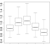
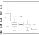
BLOCK
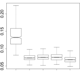
GROUP
TOEP-
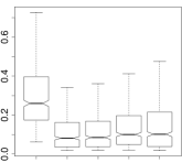
	L L+O L+R L+A L&A	L L+O L+R L+A L&A	L L+O L+R L+A L&A

Figure 1: Mean prediction error computed over 500 simulations for each design. Lasso direct estimation (L) is compared to: Lasso screening followed by OLS estimation (L+O), Lasso screening followed by ridge estimation (L+R), Lasso screening followed by adaptive-ridge estimation (L+A), jointly optimized Lasso screening with adaptive-ridge estimation (L&A).

There is no benefit in a post-Lasso estimation step for high an medium noise levels ($\operatorname{SNR}\in\{4,8\}$). OLS and ridge post-processing then have important detrimental effects and adaptive ridge has still a slight unfavorable effect. It is only when the two-step procedure is jointly optimized with respect to the two penalization parameters (by cross-validation), that some improvements become visible for the first three setups.

When the signal-to-noise ratio is high ($\operatorname{SNR}=32$), Lasso highly benefits from the second stage whatever it may be (OLS, ridge or adaptive-ridge). There is a slight edge to adaptive ridge when variables are independent, but otherwise all methods are at par. Globally, the best option here consists again in jointly optimizing the two stages with respect to the two penalization parameters; some additional improvements come into view.

Compared to previous studies, which mainly focused on large sample and/or low-noise settings, our experiments demonstrate that post-Lasso estimation can have consequential beneficial or detrimental effects in small sample regression. In addition to the experimental design, the results vary also considerably according to the strategy governing the choice of the penalty parameters. Other experiments (not shown here) attest that using more stringent screening stages (using the so-called “1-SE rule” of Breiman et al. 1984, that chooses the highest penalty within one standard deviation of the minimum of cross-validation) lead to better post-Lasso estimation in some experimental setups, but this is not systematic: in the TOEP^- design, this is by far the least favorable option. Overall, the joint optimization with respect to the two penalization parameters seems to be a very challenging contender. This is also true when the Lasso screening is followed by OLS or ridge regression. The joint optimization of penalization parameter favors a stringent Lasso screening compared to the strategy based on serial cross-validation, and a less stringent one compared to the 1-SE rule. Though this solution is the most expensive from the computational viewpoint, it seems to be also the most effective one regarding predictive mean squared error.

5.3 Two-Stage Inference

In the following, we discuss the IND BLOCK, GROUP and TOEP^- designs with $n=250$, $p=500$, $|\mathcal{S}^{\star}|=25$, $\rho=0.5$ and $\operatorname{SNR}=4$, since the relative behavior of all methods is representative of the general pattern that we observed across all simulation settings. These setups lead to feasible but challenging problems for model selection.

All variants of the screen and clean procedure are evaluated here with respect to their sensitivity ($\operatorname{SEN}$), for a controlled false discovery rate $\operatorname{FDR}$. These two measures are the analogs of power and significance in the single hypothesis testing framework:

$$\operatorname{SEN}=\mathbb{E}\left[\dfrac{TP}{TP+FN}\mathbb{I}_{\{(TP+FN)>0\}}\right]\enspace,\enspace\operatorname{FDR}=\mathbb{E}\left[\dfrac{FP}{TP+FP}\mathbb{I}_{\{(TP+FP)>0\}}\right]\enspace,$$

where $FP$ is the number of false positives, $TP$ is the number of true positives and $FN$ is the number of false negatives.

We first show the importance of the cleaning stage for $\operatorname{FDR}$ control. We then show the benefits of our proposal compared to the original procedure of Wasserman and Roeder (2009) and to the univariate approach. The variable selection method of Lockhart et al. (2014) was not included in these experiments, because it did not produce convincing results in these small $n$ large $p$ designs where the noise variance is not assumed to be known.

Importance of the Cleaning Stage

Table 2 shows that the cleaning step is essential to control the $\operatorname{FDR}$ at the desired level.

Table 2: False discovery rate $\operatorname{FDR}$ and sensitivity $\operatorname{SEN}$, computed over 500 simulations for each design. The screening stage (before cleaning) is not calibrated; the cleaning stage is calibrated to control the $\operatorname{FDR}$ below $5\%$, using the Benjamini-Hochberg procedure. Our adaptive-ridge (AR) cleaning is compared with the original (OLS) cleaning and univariate testing (Univar).

Simulation design		IND		BLOCK		GROUP		TOEP-
		$\operatorname{FDR}$	$\operatorname{SEN}$	$\operatorname{FDR}$	$\operatorname{SEN}$	$\operatorname{FDR}$	$\operatorname{SEN}$	$\operatorname{FDR}$	$\operatorname{SEN}$
Before cleaning		76.7	87.5	76.0	83.9	38.9	86.2	79.9	56.5
AR cleaning		4.2	76.1	2.8	64.8	1.7	37.7	4.3	39.6
OLS cleaning		3.9	48.3	3.1	37.1	2.5	17.9	3.7	25.3
Univar		4.4	40.4	86.4	71.0	5.3	100.0	4.2	28.4

In the screening stage, the variables selected by the Lasso are way too numerous: first, the penalty parameter is determined to optimize the cross-validated mean squared error, which is not optimal for model selection; second, we are far from the asymptotic regime where support recovery can be achieved. As a result, the Lasso performs rather poorly. Cleaning enables the control of the $\operatorname{FDR}$, leading of course to a decrease in sensitivity, which is moderate for independent variables, and higher in the presence of correlations.

Comparisons of Controlled Selection Procedures

Figure 2 provides a global picture of sensitivity according to $\operatorname{FDR}$, for the test statistics computed in the cleaning stage.

	IND		BLOCK
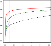
$\operatorname{SEN}$		$\operatorname{SEN}$
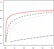
	$\operatorname{FDR}$		$\operatorname{FDR}$
	GROUP		TOEP-
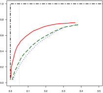
$\operatorname{SEN}$		$\operatorname{SEN}$
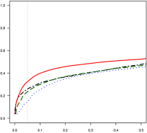
	$\operatorname{FDR}$		$\operatorname{FDR}$

Figure 2: Sensitivity $\operatorname{SEN}$ versus False Discovery Rate $\operatorname{FDR}$ (the higher, the better). Lasso screening followed by: adaptive-ridge cleaning (red solid line), ridge cleaning (green dashed line), OLS cleaning (blue dotted line); univariate testing (black dot-dashed line). All curves are indexed by the rank of the test statistics, and averaged over the $500$ simulations of each design. The vertical dotted line marks the 5% $\operatorname{FDR}$ level.

First, we observe that the direct univariate approach, which simply considers a $t$-statistic for each variable independently, is by far the worst option in the IND, BLOCK and TOEP^- designs, and by far the best in the GROUP design. In this last situation, the univariate approach confidently detects all the correlated variables of the relevant group, while the regression-based approaches are hindered by the high level of correlation between variables. Betting on the univariate approach may thus be profitable, but it is also risky due to its extremely erratic behavior. Second, we see that our adaptive-ridge cleaning systematically dominates the original OLS cleaning. To isolate the effect of transfering the magnitude of weights from the effect of the regularization brought by adaptive-ridge, we show the results obtained from a cleaning step based on plain ridge regression (with regularization parameter set by cross-validation). We see that ridge regression cleaning improves upon OLS cleaning, but that adaptive-ridge cleaning brings this improvement much further, thus confirming the value of the weight transfer from the screening stage to the cleaning stage.

Table 2 shows the actual operating conditions of the variable selection procedures, when a threshold on the test statistics has to be set to control the $\operatorname{FDR}$. Here, the threshold is set to control the $\operatorname{FDR}$ at a $5\%$ level, using a Benjamini-Hochberg correction. This control is always effective for the screen and clean procedures, but not for variable selection based on univariate testing. In all designs, our proposal dramatically improves over the original OLS strategy, with sensitivity gains ranging from $50\%$ to $100\%$. All differences in sensitivity are statistically significant. The variability of $\operatorname{FDR}$ and sensitivity is not shown to avoid clutter, but the smallest variability in $\operatorname{FDR}$ is obtained for the adaptive-ridge cleaning, while the smallest variability in sensitivity is obtained for univariate regression, followed by adaptive-ridge cleaning. The adaptive ridge penalty thus brings about more stability to the overall selection process.

6 Discussion

We propose to use the magnitude of regression coefficients in two-stage variable selection procedures. First, we use the connection between the Lasso and adaptive-ridge (Grandvalet 1998) to convey more information from the screening stage to the second stage: the magnitude of the coefficients estimated at the screening stage is transferred to the second stage through penalty parameters.

Empirically, our procedure brings marginal improvements when the second stage aims at improving the regression coefficients (Belloni and Chernozhukov 2013, Liu and Yu 2013), and it provides sensible improvements compared to the original screen and clean procedure (Wasserman and Roeder 2009) when assessing the uncertainties pertaining to the selection of relevant variables. In the first setup, screening and estimation are performed on the same data set, whereas in the second one, the screening and cleaning stages operate on two distinct subsamples of data: the transfer is more valuable in this situation.

Regarding post-Lasso estimation, our experiments demonstrate that two-stage methods can have consequential beneficial or detrimental effects in small sample regression. The results vary considerably according to the strategy governing the choice of the penalty parameters, but the joint optimization with respect to the two penalization parameters is the most effective one regarding predictive mean squared error.

For screen and clean, we obtained a better control of the False Discovery Rate, which extends to more difficult settings, with high correlations between variables. Furthermore, the sensitivity obtained by our cleaning stage is always as good, and often much better than the one based on the ordinary least squares. The penalized second step also allows for a less severe screening, since the second stage can then handle more than $n/2$ variables. Our procedure can thus be employed in very high-dimensional settings, as the screening property (that is, in the words of Bühlmann (2013), the ability of the Lasso to select all relevant variables) is more easily fulfilled, which is essential for a reliable control of the false discovery rate.

Several interesting directions are left for future works. The second stage can accommodate arbitrary penalties, and our efficient implementation applies to all penalties for which a quadratic variational formulation can be derived. This is particularly appealing for structured penalties such as the fused-lasso or the group-Lasso, allowing to use the knowledge of groups at the second stage, through penalization coefficients.

On the theoretical side, many interesting issues are raised. In particular, we would like to back-up the empirical improvements that have been almost systematically observed by an apposite analysis. We believe that two tracks are promising: first by exploiting that the screening stage transfers a quantified response to the cleaning stage through the penalization coefficients, and second, that screening needs not to be stringent, due to the ability of our second stage to handle more variables.

Software

Software and simulations are in the form of R package named “ridgeAdap” available on the personal author page (https://www.hds.utc.fr/~becujean).

Acknowlegements

This work was supported by the UTC foundation for Innovation, in the ToxOnChip program. It has been carried out in the framework of the Labex MS2T (ANR-11-IDEX-0004-02) within the “Investments for the future” program, managed by the National Agency for Research.

Appendix A Variational Equivalence

We show below that the quadratic penalty in $\boldsymbol{\beta}$ in Problem (2) acts as the Lasso penalty $\lambda\left\|\boldsymbol{\beta}\right\|_{1}$.

Proof.

The Lagrangian of Problem (2) is:

$$L(\boldsymbol{\beta})=J(\boldsymbol{\beta})+\lambda\sum_{j=1}^{p}\frac{1}{\tau_{j}}\beta_{j}^{2}+\nu_{0}\bigg{(}\sum_{j=1}^{p}\tau_{j}-\left\|\boldsymbol{\beta}\right\|_{1}\bigg{)}-\sum_{j=1}^{p}\nu_{j}\tau_{j}\enspace.$$

Thus, the first order optimality conditions for $\tau_{j}$ are

$$\frac{\partial L}{\partial\tau_{j}}(\tau_{j}^{\star})=0 \Leftrightarrow-\lambda\frac{\beta_{j}^{2}}{{\tau_{j}^{\star}}^{2}}+\nu_{0}-\nu_{j}=0$$

$$\Leftrightarrow-\lambda\beta_{j}^{2}+\nu_{0}\,{\tau_{j}^{\star}}^{2}-\nu_{j}\,{\tau_{j}^{\star}}^{2}=0$$

$$\Rightarrow-\lambda\beta_{j}^{2}+\nu_{0}\,{\tau_{j}^{\star}}^{2}=0\enspace,$$

where the term in $\nu_{j}$ vanishes due to complementary slackness, which implies here $\nu_{j}\tau_{j}^{\star}=0$. Together with the constraints of Problem (2), the last equation implies $\tau_{j}^{\star}=\left|\beta_{j}\right|$, hence Problem (2) is equivalent to

$$\min_{\boldsymbol{\beta}\in\mathbb{R}^{p}}J(\boldsymbol{\beta})+\lambda\left\|\boldsymbol{\beta}\right\|_{1}\enspace,$$

which is the original Lasso formulation. ∎

Appendix B Efficient Implementation

Permutation tests rely on the simulation of numerous data sampled under the null hypothesis distribution. The number of replications must be important to estimate the rather extreme quantiles we are typically interested in. Here, we use $B=1000$ replications for the $q=|\mathcal{S}_{\hat{\lambda}}|$ variables selected in the screening stage. Each replication involving the fitting of a model, the total computational cost for solving these $B$ systems of size $q$ on the $q$ selected variables is $O(Bq(q^{3}+q^{2}n))$. In the situation where $q\ll B$, great computing savings can be obtained using block-wise decompositions and inversions.

First, we recall that the adaptive-ridge estimate, computed at the cleaning stage, is computed as

$$\,\hat{\!\boldsymbol{\beta}}=\left({\mathbf{X}}^{\top}\mathbf{X}+\boldsymbol{\Lambda}\right)^{-1}\mathbf{X}^{\top}\mathbf{y}\enspace,$$

where $\boldsymbol{\Lambda}$ is the diagonal adaptive-penalty matrix defined at the screening stage, whose $j$th diagonal entry is ${\lambda}/{\tau_{j}^{\star}}$, as defined in (1–3).

In the $F$-statistic (4), the permutation affects the calculation of the larger model $\hat{\mathbf{y}}_{1}$, which is denoted $\hat{\mathbf{y}}_{1}^{(b)}$ for the $b$th permutation. Using a similar notation convention for the design matrix and the estimated parameters, we have $\hat{\mathbf{y}}_{1}^{(b)}={\mathbf{X}^{(b)}}\hat{\boldsymbol{\beta}}^{(b)}$. When testing the relevance of variable $j$, ${\mathbf{X}^{(b)}}$ is defined as the concatenation of the permuted variable $\mathbf{x}_{j}^{(b)}$ and the other original variables: ${\mathbf{X}^{(b)}}=(\mathbf{x}_{j}^{(b)},\mathbf{x}_{1},...,\mathbf{x}_{j-1},\mathbf{x}_{j+1},...\mathbf{x}_{p})$. Then, $\hat{\boldsymbol{\beta}}^{(b)}$ can be efficiently computed by using $a^{(b)}\in\mathbb{R}$, $\mathbf{X}_{\fgebackslash j}\in\mathbb{R}^{q-1}$ and $\hat{\boldsymbol{\beta}}_{\fgebackslash j}\in\mathbb{R}^{q-1}$ defined as follows:

$$a^{(b)} =(\|\mathbf{x}_{j}^{(b)}\|^{2}_{2}+\Lambda_{jj})-{\mathbf{x}_{j}^{(b)}}^{\top}\mathbf{X}_{\fgebackslash j}{(\mathbf{X}_{\fgebackslash j}^{\top}\mathbf{X}_{\fgebackslash j}+{\boldsymbol{\Lambda}_{\fgebackslash j}})}^{-1}\mathbf{X}_{\fgebackslash j}^{\top}\mathbf{x}_{j}^{(b)}$$

$$\mathbf{v}^{(b)} =-{(\mathbf{X}_{\fgebackslash j}^{\top}\mathbf{X}_{\fgebackslash j}+{\boldsymbol{\Lambda}_{\fgebackslash j}})}^{-1}\mathbf{X}_{\fgebackslash j}^{\top}\mathbf{x}_{j}^{(b)}$$

$$\hat{\boldsymbol{\beta}}_{\fgebackslash j} ={(\mathbf{X}_{\fgebackslash j}^{\top}\mathbf{X}_{\fgebackslash j}+{\boldsymbol{\Lambda}_{\fgebackslash j}})}^{-1}\mathbf{X}_{\fgebackslash j}^{\top}\mathbf{y}\enspace.$$

Indeed, using the Schur complement, one writes $\hat{\boldsymbol{\beta}}^{(b)}$ as follows:

$$\hat{\boldsymbol{\beta}}^{(b)}=\frac{1}{a^{(b)}}\begin{pmatrix}1\\ \mathbf{v}^{(b)}\end{pmatrix}\begin{pmatrix}1&{\mathbf{v}^{(b)}}^{\top}\end{pmatrix}\begin{pmatrix}{\mathbf{x}_{j}^{(b)}}^{\top}\mathbf{y}\\ \mathbf{X}_{\fgebackslash j}^{\top}\mathbf{y}\end{pmatrix}+\begin{pmatrix}0\\ \hat{\boldsymbol{\beta}}_{\fgebackslash j}\end{pmatrix}\enspace.$$

Hence, $\hat{\boldsymbol{\beta}}^{(b)}$ can be obtained as a correction of the vector of coefficients $\hat{\boldsymbol{\beta}}_{\fgebackslash j}$ obtained under the smaller model. The key observation to be made here is that $\mathbf{x}_{j}^{(b)}$ does not intervene in the expression ${(\mathbf{X}_{\fgebackslash j}^{\top}\mathbf{X}_{\fgebackslash j}+{\boldsymbol{\Lambda}_{\fgebackslash j}})}^{-1}$ , which is the bottleneck in the computation of $a^{(b)}$, $\mathbf{v}^{(b)}$ and $\hat{\boldsymbol{\beta}}_{\fgebackslash j}$. It can therefore be performed once for all permutations. Additionally, ${(\mathbf{X}_{\fgebackslash j}^{\top}\mathbf{X}_{\fgebackslash j}+{\boldsymbol{\Lambda}_{\fgebackslash j}})}^{-1}$ can be cheaply computed from $\left({\mathbf{X}}^{\top}\mathbf{X}+\boldsymbol{\Lambda}\right)^{-1}$ as follows:

$${(\mathbf{X}_{\fgebackslash j}^{\top}\mathbf{X}_{\fgebackslash j}+{\boldsymbol{\Lambda}_{\fgebackslash j}})}^{-1}= \left[\left({\mathbf{X}}^{\top}\mathbf{X}+\boldsymbol{\Lambda}\right)^{-1}\right]_{\fgebackslash j\fgebackslash j}-$$

$$\left[\left({\mathbf{X}}^{\top}\mathbf{X}+\boldsymbol{\Lambda}\right)^{-1}\right]_{\fgebackslash jj}\left[\left({\mathbf{X}}^{\top}\mathbf{X}+\boldsymbol{\Lambda}\right)^{-1}\right]_{jj}^{-1}\left[\left({\mathbf{X}}^{\top}\mathbf{X}+\boldsymbol{\Lambda}\right)^{-1}\right]_{j{\fgebackslash j}}\enspace.$$

Thus we compute $\left({\mathbf{X}}^{\top}\mathbf{X}+\boldsymbol{\Lambda}\right)^{-1}$ once, firstly correct for the removal of variable $j$, secondly correct for permutation $b$, thus eventually requiring $O(B(q^{3}+q^{2}n)))$ operations.

References

- Ambroise and McLachlan (2002) C. Ambroise and G. J. McLachlan. Selection bias in gene extraction on the basis of microarray gene-expression data. Proceedings of the National Academy of Sciences, 99(10):6562–6566, 2002.
- Anders and Huber (2010) S. Anders and W. Huber. Differential expression analysis for sequence count data. Genome Biology, 11(10):R106, 2010.
- Bach et al. (2012) F. Bach, R. Jenatton, J. Mairal, and G. Obozinski. Optimization with sparsity-inducing penalties. Foundations and Trends in Machine Learning, 4(1):1–106, 2012.
- Balding (2006) D. Balding. A tutorial on statistical methods for population association studies. Nature Reviews Genetics, 7(10):781–791, october 2006.