NLO QCD corrections to the resonant Vector Diquark production at the LHC

Abstract

With the upcoming run of the Large Hadron Collider (LHC) at much higher center of mass energies, the search for Beyond Standard Model (BSM) physics will again take center stage. New colored particles predicted in many BSM scenarios are expected to be produced with large cross sections thus making them interesting prospects as a doorway to hints of new physics. We consider the resonant production of such a colored particle, the diquark, a particle having the quantum number of two quarks. The diquark can be either a scalar or vector. We focus on the vector diquark which has much larger production cross section compared to the scalar ones. In this work we calculate the next-to-leading order (NLO) QCD corrections to the on-shell vector diquark production at the LHC produced through the fusion of two quarks as well as the NLO corrections to its decay width. We present full analytic results for the one-loop NLO calculation and do a numerical study to show that the NLO corrections can reduce the scale uncertainties in the cross sections which can be appreciable and therefore modify the expected search limits for such particles. We also use the dijet result from LHC to obtain current limits on the mass and coupling strengths of the vector diquarks.

1 Introduction

After the successful running of the Large Hadron Collider (LHC) at CERN with 7 and 8 TeV center of mass energies, the data released by the two experiments, ATLAS and CMS have not only improved on the limits set by the Tevatron experiments on any new physics scenario, but has also started giving some insights into the TeV scale. In addition to the observation of a scalar resonance at 125 GeV Aad:2012tfa ; Chatrchyan:2012ufa consistent with that of the Standard Model (SM) like Higgs boson, the results are also in very good agreement with predictions from the SM, with not much deviation. This means that the LHC data is already pushing the energy frontier of any Beyond Standard Model (BSM) physics predictions. However with the upgraded run of LHC at center of mass energy of 13 TeV and subsequently 14 TeV, the search for new physics is expected to be more robust and as envisaged for the LHC run. As expected and observed from the previous LHC runs, the data would be most sensitive to the strongly interacting sector through production of new colored states. Since the initial states at hadron colliders such as the LHC are colored particles, the most dominant contributions would be through new colored resonances. Such colored particles are predicted in many class of BSM theories. Resonant s-channel production at LHC can happen for squarks in R-Parity violating supersymmetric theories Barbier:2004ez , diquarks in super-string inspired $E_{6}$ grand unification models Hewett:1988xc or models with extended gauge symmetries Chakdar:2013haa ; Chakdar:2012vv ; Li:2012zy , color-octet vectors such as axigluons Frampton:1987dn ; Bagger:1987fz and colorons Hill:1991at ; Hill:1993hs ; ddn:1995pr ; Sayre:2011ed , models with color-triplet Babu:2006wz , color-sextet Pati:1974yy ; Mohapatra:1980qe ; Chacko:1998td or color-octet scalars Hill:2002ap ; Dobrescu:2007yp . The absence of any such observation in the existing data put strong limits on such particle masses, from pair production of such states, or more strongly from resonant searches of new physics exchanged in the s-channel Harris:2011bh .

These resonant colored states are most likely to decay to two light jets leading to not only the modification of the dijet differential cross section at large invariant mass but also show up as a bump in its invariant mass distribution. Such a signal will not go unnoticed and will be fairly very distinct at large invariant mass values, as the significantly huge QCD background falls rapidly for large dijet invariant mass. Both ATLAS and CMS Collaborations have looked at the dijet signal and already put strong constraints on the mass of such resonances Aad:2010bc ; Aad:2011bc ; Aad:2014bc ; Khachatryan:2010jd ; Chatrchyan:2011ns ; Khachatryan:2015jd . We should however note that the production of such colored particles will be beset with significant contributions from QCD corrections, and therefore it becomes important to understand how much the leading order (LO) rates might change once these corrections are included. One finds that there have been significant efforts in this direction to study the next-to-leading order (NLO) QCD effects on production of some of the new colored particles Han:2009ya ; Chivukula:2011ng ; Chivukula:2013xla arising in BSM at the LHC. Here we are interested in particular with particles of the “diquark” type which carry non-zero baryon number and couple to a pair of quarks or anti-quarks. The fact that LHC being a proton-proton collider will have valence quarks in much abundance compared to the anti-quarks, helps in producing the diquark as a resonance through $qq$ fusion. A lot of studies carried out at LO exist in the literature for such diquarks and their resonant effects in the dijet signal Atag:1998xq ; Arik:2001bc ; Cakir:2005iw ; Mohapatra:2007af ; Berger:2010fy ; Han:2010rf ; Giudice:2011ak ; Richardson:2011df , pair production of top quarks Barger:2006hm ; Frederix:2007gi ; Zhang:2010kr ; Kosnik:2011jr and single top quark production at the LHC Gogoladze:2010xd ; Karabacak:2012rn . The one-loop NLO correction for scalar diquark production was considered in Ref Han:2009ya . We focus on the case of vector diquarks which are either antitriplets or sextets of $SU(3)_{C}$. Such particles will also be copiously produced as s-channel resonances with much larger cross section compared to the scalar ones. Once produced, the vector diquark will decay and would thus contribute to the dijet final state or to final states involving the third-generation quarks.

For our study of estimating the NLO corrections to the on-shell production of a vector diquark at the LHC, we follow in part the methodology used in Ref Han:2009ya to present our results. In Sec. 2 we present the formalism and give the basic interaction Lagrangian relevant for our study and in Sec. 3 we discuss the on-shell production cross section of the vector diquark, and present our calculations and analytic expressions for the NLO QCD results. In Sec. 4 we give results for the one-loop corrections to the decay width of the vector diquark. In Sec. 5 we give our numerical results for the NLO cross sections and its dependence on the choice of scale for the production of the vector diquark in different channels at the LHC. We also consider its effect on the experimental limits for such particles and finally in Sec. 6 we give our conclusions with future outlook. Some relevant formulas are collected as an Appendix.

2 Formalism

We are interested in new colored particles that couple to a pair of quarks directly and carry exotic baryon number. With the LHC being a proton-proton machine, the initial states comprised of the the valence quarks ($u,d$) would lead to enhanced flux in the parton distributions for the collision between a pair of valence quarks such as $uu,dd$ or $ud$. Any new particle that couples to these pairs would carry a baryon number $B=\dfrac{2}{3}$ and will be charged under the SM color gauge group $SU(3)_{C}$. Such states are generally referred to as diquarks. These colored diquarks can be either color antitriplets or sextets of $SU(3)_{C}$. We can describe the vector diquarks following Ref Karabacak:2012rn according to color representation ($\bar{\mathbf{3}},\ \mathbf{6}$) and electric charge ($4/3,\ 2/3,\ 1/3$) as $V_{2\cal U}^{N_{D}},V_{\cal U}^{N_{D}},V_{\cal D}^{N_{D}}$, where the subscripts $2{\cal U},{\cal U}$, and ${\cal D}$ in the fields indicate their electric charge $|Q|$ of two up type quarks, one up and one down type quark respectively, while $N_{D}(=3~{}(6))$ is the dimension of the antitriplet (sextet) representation. The relevant interactions of the quarks with the different vector diquarks is given by the Lagrangian

$$\begin{multlined}\mathcal{L}_{qqD}^{V}=K_{ab}^{j}\Big{[}\frac{\lambda_{\alpha\beta}^{2{\cal U}}}{\sqrt{1+\delta_{\alpha\beta}}}V^{j\mu}_{2{\cal U}}\overline{{\cal U}^{c}}_{\alpha a}\gamma_{\mu}P_{\tau}{\cal U}_{\beta b}+\frac{\lambda_{\alpha\beta}^{\cal U}}{\sqrt{1+\delta_{\alpha\beta}}}V_{\cal U}^{j\mu}\overline{{\cal D}^{c}}_{\alpha a}\gamma_{\mu}P_{\tau}{\cal D}_{\beta b}\\ +\lambda_{\alpha\beta}^{\cal D}V_{\cal D}^{j\mu}\overline{{\cal U}^{c}}_{\alpha a}\gamma_{\mu}P_{\tau}{\cal D}_{\beta b}\Big{]}+\mathrm{h.c.}\end{multlined}\mathcal{L}_{qqD}^{V}=K_{ab}^{j}\Big{[}\frac{\lambda_{\alpha\beta}^{2{\cal U}}}{\sqrt{1+\delta_{\alpha\beta}}}V^{j\mu}_{2{\cal U}}\overline{{\cal U}^{c}}_{\alpha a}\gamma_{\mu}P_{\tau}{\cal U}_{\beta b}+\frac{\lambda_{\alpha\beta}^{\cal U}}{\sqrt{1+\delta_{\alpha\beta}}}V_{\cal U}^{j\mu}\overline{{\cal D}^{c}}_{\alpha a}\gamma_{\mu}P_{\tau}{\cal D}_{\beta b}\\ +\lambda_{\alpha\beta}^{\cal D}V_{\cal D}^{j\mu}\overline{{\cal U}^{c}}_{\alpha a}\gamma_{\mu}P_{\tau}{\cal D}_{\beta b}\Big{]}+\mathrm{h.c.}$$ (1)

where $P_{\tau}=\frac{1}{2}(1\pm\gamma_{5})$ with $\tau=L,R$ representing left and right chirality projection operators and superscript $\mu$ is the Lorentz four vector index. The $K^{j}_{ab}$ are $SU(3)_{C}$ Clebsch-Gordan coefficients with the quark color indices $a,b=1-3$, and the diquark color index $j=1-N_{D}$, $C$ denotes charge conjugation, while $\alpha,\beta$ are the fermion generation indices. The color factor $K^{j}_{ab}$ is symmetric (antisymmetric) under $ab$ for the ${\mathbf{6}}\ (\bar{\mathbf{3}})$ representation. A more general form of the Lagrangian can be found in Ref Han:2010rf . A factor of $1/\sqrt{2}$ in the interaction terms involving same quark flavors is introduced to keep the expressions for the production cross section as well as the decay width same for both different flavor and same flavor cases. To calculate the QCD corrections to the diquark production, we also need to know how the vector diquark ($V_{i}^{\mu}$) interacts with the gluons, which is given by the Lagrangian,

$${\cal L}^{V}_{GDD} = -\frac{1}{2}(V_{i\mu\nu})^{\dagger}(V_{i}^{\mu\nu})-ig_{s}\;V_{i\mu}^{\dagger}T^{A}_{ij}V_{j\nu}G^{A,\mu\nu}$$ (2)

where,

$$V_{i}^{\mu\nu} = D^{\mu}_{ij}V_{j}^{\nu}-D^{\nu}_{ij}V_{j}^{\mu}$$ (3)

$$G^{A}_{\mu\nu} = \partial_{\mu}G^{A}_{\nu}-\partial_{\nu}G^{A}_{\mu}+g_{s}f^{ABC}G^{B}_{\mu}G^{C}_{\nu}$$ (4)

$$D_{\mu,ij} \equiv \delta_{ij}\partial_{\mu}-ig_{s}\;G^{A}\mu T^{A}_{ij}.$$ (5)

The indices $i$ and $j$ again run from $1\to N_{D}$, where $N_{D}$ is the dimension of the diquark representation. The index $A$ runs from $1\to 8$ and $T^{A}_{ij}$ are the $SU(3)_{C}$ generators in the diquark representation. Note that we have suppressed the electric charge index ($2\cal U,U,D$) for the diquark as we are interested only in the QCD corrections. The Feynman rules for three-point vertices involving vector diquark are given in Appendix A.

The diquark can couple to the initial state valence partons coming from both the protons, and the production of the diquark would get significant enhancement due to the large flux of the valence quarks in the proton. Therefore the production rates are only constrained by its coupling strength to the pair of initial quarks and its mass, which are the two free parameters in our analysis. Moreover, it is also equally probable that the vector diquarks have generation dependent couplings following Eq. 1. Therefore the couplings ($\lambda^{2\cal U},\lambda^{\cal U},\lambda^{\cal D}$) involved in Eq. 1 are completely arbitrary and can in principle be large. Note that most of them are tightly constrained by flavor physics as they might mediate light meson or hadron decays Barbier:2004ez ; Han:2009ya . Therefore the constraints on the interaction of the vector diquark with the lighter quarks (first and second generation) are much more stronger, which means that vector diquark production at the LHC can have different allowed interaction strengths depending on the initial quarks participating in the production. To make our analysis more general we therefore choose to present our results normalized to the coupling strength. Where applicable, we would also assume that we work in the minimal flavor violating (MFV) scheme D'Ambrosio:2002ex for the couplings involving both the left- and right-chiral quarks with the vector diquark. It is worth noting that these colored states do not have direct coupling to a pair of gluons and thus the production cross section for diquark is limited by the flux of the initial partons in the proton at the LHC. However large QCD corrections can significantly alter the rates and modify the existing constraints on the mass and interaction strengths of such colored states. In this work we have chosen to ignore any electroweak corrections as interactions of the vector diquark to the electroweak gauge bosons might be model dependent.

3 Production cross section at next-to-leading order

We shall work in the “narrow-width” approximation where we can write the cross section as a product of the on-shell production and decay of the vector diquark ($V_{D}$) in a particular channel $(XX)$ as

$$\sigma\left(pp\to XX\right)\simeq\sigma\left(pp\to V_{D}\right)\times\frac{\Gamma(V_{D}\to XX)}{\Gamma(V_{D}\to all)}$$ (6)

Thus $\sigma\left(pp\to V_{D}\right)$ gives the cross section for the production of the diquark resonance. The leading order or Born contribution to the on-shell vector diquark production comes from quark-quark initial states. The relevant Feynman diagram is shown in Fig.1.

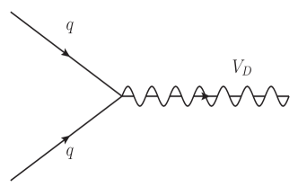
Figure 1: Feynman diagram at Born level for the process $qq\rightarrow V_{D}.$

For the diquark of mass $M_{D}$, the parton-level cross section at the LO is given by

$$\hat{\sigma}_{\rm B} = \frac{\hat{\sigma}_{0}}{\hat{s}}\;\delta(1-\tau),$$ (7)

where

$$\hat{\sigma}_{0}=\frac{\lambda^{2}\pi N_{D}}{2N_{C}^{2}}.$$ (8)

In the above, $\hat{s}$ is the partonic center of mass energy, $N_{C}=3$ is the color factor of the quarks and $\tau=M_{D}^{2}/\hat{s}$. It is useful to rewrite the LO cross section in $n=4-2\epsilon$ dimensional form as this $n$-dimensional result will be used in the NLO calculation. Thus Eq. 8 can be put in the form

$$\hat{\sigma}_{0}=\frac{(n-2)\pi N_{D}\lambda^{2}(\mu^{2})\mu^{2\epsilon}}{4N_{C}^{2}}.$$ (9)

Here $\lambda(\mu^{2})$ represents the running coupling parameter and $\mu$ defines the scale introduced to make the coupling dimensionless. From here onwards we shall drop the various indices from the coupling parameter introduced in the Lagrangian 1. The corresponding hadronic cross section at colliders can be obtained by convoluting the parton-level cross section with the parton distribution functions (PDF) of the initial quarks participating in the production, i.e.

$$\sigma_{\rm LO}=\frac{\hat{\sigma}_{0}}{s}~{}(q\otimes q)(\tau_{0}),$$ (10)

where $s$ is the hadronic center of mass energy and $\tau_{0}=M_{D}^{2}/s$. We have used the notation for convolution of two functions, defined by

$$(f_{1}\otimes f_{2})(x_{0})=\int_{0}^{1}dx_{1}\int_{0}^{1}dx_{2}~{}\delta(x_{1}x_{2}-x_{0})f_{1}(x_{1})f_{2}(x_{2}).$$ (11)

Although the LO process involves colored particles only, the interaction strength does not involve the strong coupling $g_{s}$ but only the coupling strengths given by the free parameter $\lambda$. Therefore the one-loop QCD corrections at NLO are in leading order of $\alpha_{s}=\frac{g_{s}^{2}}{4\pi}$. The ${\cal O}(\alpha_{s})$ QCD correction to the vector diquark production involves :

• Virtual corrections due to one-loop gluon contributions.

• Real corrections due to the gluon emission from initial state quarks and final state diquark.

• For the complete ${\cal O}(\alpha_{s})$ correction, one also needs to consider quark-gluon initiated diquark production with a jet.

We use dimensional regularization (DR) to regulate the ultraviolet (UV) and infrared (IR) singularities that may appear in these corrections. The renormalization of UV singularity and factorization of collinear singularity is carried out in the $\overline{\rm MS}$ scheme. We have performed various checks, including the gauge invariance check with respect to the gluon at the amplitude and amplitude-squared levels, to ensure the correctness of our calculations.

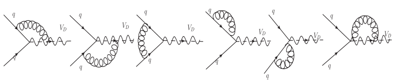
Figure 2: Feynman diagrams for virtual gluon correction to the process $qq\rightarrow V_{D}.$

3.1 Virtual corrections

The virtual corrections at ${\cal O}(\alpha_{s})$ come from the interference of Born and one-loop amplitudes. The one-loop diagrams contributing to virtual corrections are displayed in Fig. 2. These diagrams are both UV and IR divergent. The required one-loop computation is carried out following the standard method of one-loop tensor reduction in $n=4-2\epsilon$ dimensions. We have listed all the one-loop scalar functions that we have used in the calculation, in Appendix B. The virtual cross section coming from vertex correction diagrams is given by,

$$\begin{multlined}\hat{\sigma}_{\rm V}=\hat{\sigma}_{\rm B}\frac{\alpha_{s}C_{\epsilon}}{2\pi}\Big{[}C_{D}\Big{\{}\frac{8}{3}{1\over\epsilon_{\rm UV}}-\frac{2\pi^{2}}{3}+{77\over 18}\Big{\}}+C_{F}\Big{\{}\frac{1}{\epsilon_{\rm UV}}-\frac{2}{\epsilon_{\rm IR}^{2}}-\frac{4}{\epsilon_{\rm IR}}+\pi^{2}-8\Big{\}}\Big{]}.\end{multlined}\hat{\sigma}_{\rm V}=\hat{\sigma}_{\rm B}\frac{\alpha_{s}C_{\epsilon}}{2\pi}\Big{[}C_{D}\Big{\{}\frac{8}{3}{1\over\epsilon_{\rm UV}}-\frac{2\pi^{2}}{3}+{77\over 18}\Big{\}}+C_{F}\Big{\{}\frac{1}{\epsilon_{\rm UV}}-\frac{2}{\epsilon_{\rm IR}^{2}}-\frac{4}{\epsilon_{\rm IR}}+\pi^{2}-8\Big{\}}\Big{]}.$$ (12)

The overall factor $C_{\epsilon}=\frac{1}{\Gamma(1-\epsilon)}\Big{(}\frac{4\pi\mu^{2}}{\hat{s}}\Big{)}^{\epsilon}$ appears in all one-loop integrals regulated in DR. $C_{F}$ and $C_{D}$ are the eigenvalues of the quadratic Casimir operator of $SU(3)_{C}$ acting on the fundamental representation and on the diquark representation respectively. For both the sextet and antitriplet diquark, $C_{F}=4/3$ while $C_{D}$ is $4/3$ for the antitriplet and $10/3$ for the sextet diquark. The effect of external leg corrections can be incorporated in the wave function renormalization of the quark and diquark fields. Thus one can conveniently express the sum of Born and virtual cross section to ${\cal O}({\alpha_{s}})$ as muta ,

$$\hat{\sigma}_{\rm{B+V}}=(Z_{2}^{q})^{2}Z_{2}^{D}\hat{\sigma}_{\rm B}+\hat{\sigma}_{\rm V}.$$ (13)

The wave function renormalization constants $Z_{2}^{q}$ and $Z_{2}^{D}$ for quark and vector diquark fields are,

$$Z_{2}^{q} = 1+\frac{\alpha_{s}}{4\pi}C_{\epsilon}\;C_{F}\Big{(}-\frac{1}{\epsilon_{\rm UV}}+\frac{1}{\epsilon_{\rm IR}}\Big{)}$$ (14)

$$Z_{2}^{D} = 1+\frac{\alpha_{s}}{4\pi}C_{\epsilon}\;C_{D}\Big{(}\frac{2}{\epsilon_{\rm UV}}-\frac{2}{\epsilon_{\rm IR}}\Big{)}.$$ (15)

Note that these renormalization constants are calculated for on-shell quark and diquark fields, therefore, the IR singularity also appears. In DR, both are one as $\epsilon_{\rm UV}=\epsilon_{\rm IR}=\epsilon$. However, the above form is suitable for extracting the full UV singularity in virtual corrections. The sum of Born and virtual cross section thus becomes,

$$\begin{multlined}\hat{\sigma}_{\rm{B+V}}=\hat{\sigma}_{\rm B}\Bigg{[}1+\frac{\alpha_{s}C_{\epsilon}}{2\pi}\Big{\{}C_{F}\Big{[}-\frac{2}{\epsilon_{\rm IR}^{2}}-\frac{3}{\epsilon_{\rm IR}}+\pi^{2}-8\Big{]}\\ +C_{D}\Big{[}\frac{11}{3}\frac{1}{\epsilon_{\rm UV}}-\frac{1}{\epsilon_{\rm IR}}-\frac{2\pi^{2}}{3}+\frac{77}{18}\Big{]}\Big{\}}\Bigg{]}.\end{multlined}\hat{\sigma}_{\rm{B+V}}=\hat{\sigma}_{\rm B}\Bigg{[}1+\frac{\alpha_{s}C_{\epsilon}}{2\pi}\Big{\{}C_{F}\Big{[}-\frac{2}{\epsilon_{\rm IR}^{2}}-\frac{3}{\epsilon_{\rm IR}}+\pi^{2}-8\Big{]}\\ +C_{D}\Big{[}\frac{11}{3}\frac{1}{\epsilon_{\rm UV}}-\frac{1}{\epsilon_{\rm IR}}-\frac{2\pi^{2}}{3}+\frac{77}{18}\Big{]}\Big{\}}\Bigg{]}.$$ (16)

To get rid of the UV divergence in the above, renormalization of the coupling parameter $\lambda$ is necessary which is equivalent to adding an UV counter term of the following form to Eq. 16,

$$\hat{\sigma}_{\rm C.T.}^{\rm UV}=-\hat{\sigma}_{\rm B}\frac{\alpha_{s}}{2\pi}\frac{(4\pi)^{\epsilon}}{\Gamma(1-\epsilon)}C_{D}\frac{11}{3}\Big{(}\frac{1}{\epsilon_{\rm UV}}+{\rm ln}\frac{\mu^{2}}{\mu_{R}^{2}}\Big{)}$$ (17)

where $\mu_{R}$ is the renormalization scale. Hence the UV renormalized parton-level cross section to ${\cal O}(\alpha_{s})$ for the production of diquark from $qq$ initial state is given by

$$\hat{\sigma}_{\rm B+V+C.T.} = \hat{\sigma}_{\rm B}\Big{[}1+\frac{\alpha_{s}C_{\epsilon}}{2\pi}\Big{\{}C_{F}\Big{(}-\frac{2}{\epsilon_{\rm IR}^{2}}-\frac{3}{\epsilon_{\rm IR}}+\pi^{2}-8\Big{)}$$ (18)

$$+C_{D}\Big{(}-\frac{1}{\epsilon_{\rm IR}}+\frac{11}{3}{\rm ln}\frac{\mu_{R}^{2}}{\hat{s}}-\frac{2\pi^{2}}{3}+\frac{77}{18}\Big{)}\Big{\}}\Big{]}.$$

Note that the procedure of renormalization has introduced a scale dependence in the cross section which would help in reducing the overall scale dependence due to the running of the coupling. After regulating the UV divergence, we are left with IR divergences, part of which will be canceled (due to Kinoshita-Lee-Nauenberg (KLN) theorem muta ) once we take into account the real gluon emission contribution. It is important to note that the singularity structure of virtual cross section is the same in the scalar Han:2009ya and vector diquark cases. Just like the singular terms proportional to $C_{F}$, we find that the singular term proportional to $C_{D}$ is also universal.

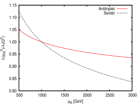
Figure 3: Running of quark-diquark coupling with respect to the renormalization scale ($\mu_{R}$) to ${\cal O}(\alpha_{s})$.

Note that the results of this section can be utilized to predict the one-loop running of the quark-quark-diquark coupling $\lambda$. The one-loop beta function due to ${\cal O}(\alpha_{s})$ QCD correction is therefore given by

$$\beta(\lambda)=\mu^{2}\frac{d{\rm ln}\lambda}{d\mu^{2}}=-\frac{\alpha_{s}}{4\pi}\Big{(}\frac{11}{3}C_{D}\Big{)}.$$ (19)

Solving this, the running of the renormalized coupling parameter $\lambda(\mu_{R}^{2})$ follows

$$\lambda(\mu_{R}^{2})=\lambda(Q^{2})\Big{[}1-\frac{\alpha_{s}(\mu_{R}^{2})}{4\pi}\frac{11}{3}C_{D}\ln\Big{(}\frac{\mu_{R}^{2}}{Q^{2}}\Big{)}\Big{]},$$ (20)

where $Q$ is a reference scale which we will identify with $M_{D}$ (mass of the vector diquark) and choose $\lambda(M_{D}^{2})=1$. It is worth pointing out that in contrast to the scalar diquark case, the one-loop running of the coupling in the vector diquark case depends on the diquark representation and therefore will behave differently for the antitriplet and the sextet. This is highlighted in Fig. 3 where we show how the coupling $\lambda$ varies as a function of the renormalization scale $\mu_{R}$. Note that we have chosen $\lambda(Q^{2})=1$ for $Q=M_{D}=1$ TeV as a reference point which is just for illustration purposes only. The scale dependence for the antitriplet vector diquark coupling is found to be at $\sim 6\%$ for the $\mu_{R}$ range considered while that for the sextet turns out to be significantly higher at $\sim 16\%$ for the same variation in $\mu_{R}$. This is due to the dependence of the one-loop beta function on $C_{D}$ which takes different values for the two cases. Note that the running of the coupling will bring in a scale dependence for the LO cross section of the diquark too, similar to that observed for QCD cross sections due to the running of the strong coupling constant $\alpha_{s}$.

3.2 Real Corrections: $qq$ channel

Next, we compute the contribution from the gluon bremsstrahlung radiated from initial state as well as final state to ${\cal O}(\alpha_{s})$. The process for the real gluon emission is,

$$q_{i}(p_{1})+q_{j}(p_{2})\rightarrow g(k)+V_{D}(p_{1}+p_{2}-k).$$

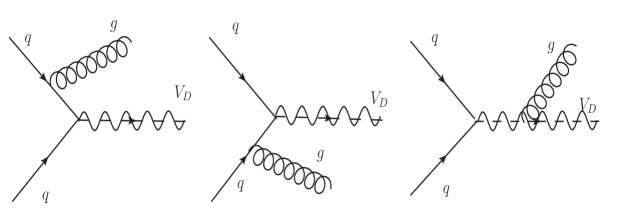
Figure 4: Feynman diagram at leading order for the process $qq\rightarrow g~{}V_{D}.$

The Feynman diagrams which contribute to the NLO level gluon emission process for diquark production is given in Fig 4. The full ${\cal O}(\alpha_{s})$ spin and color averaged squared-amplitude for the three different diagrams shown in Fig. 4 can be expressed in terms of Mandelstam variables $(s,t,u)$ in $n=4-2\epsilon$ space-time dimensions and is given by,

$$\sum\overline{|{\cal M}^{R}_{qq}|^{2}} = \frac{(n-2)N_{D}g_{s}^{2}\lambda^{2}\mu^{4\epsilon}}{4N_{C}^{2}tu(t+u)^{2}}\Big{(}-C_{D}tu+C_{F}(t+u)^{2}\Big{)}$$ (21)

$$\times \Big{(}4s^{2}+(n-2)t^{2}+2(n-4)tu+(n-2)u^{2}+4s(t+u)\Big{)}$$

where $s=(p_{1}+p_{2})^{2},\;t=(p_{1}-k)^{2}\;$ and $u=(p_{2}-k)^{2}$. The partonic cross section for the real gluon emission process is obtained by performing the phase space integration in $4-2\epsilon$ dimensions and is given by

$$\begin{multlined}\hat{\sigma}^{R}_{qq}=\frac{\hat{\sigma}_{0}}{\hat{s}}\frac{\alpha_{s}}{2\pi}C_{\epsilon}\Bigg{[}C_{F}\Bigg{\{}(\frac{2}{\epsilon_{\rm IR}^{2}}+\frac{3}{\epsilon_{\rm IR}}-\frac{\pi^{2}}{3})\delta(1-\tau)-\frac{2}{\epsilon_{\rm IR}}\left(\frac{1+\tau^{2}}{1-\tau}\right)_{+}\\ +4(1+\tau^{2})\left(\frac{{\rm ln}(1-\tau)}{1-\tau}\right)_{+}\Bigg{\}}\\ +C_{D}\Bigg{\{}(\frac{1}{\epsilon_{\rm IR}}+\frac{11}{3})\delta(1-\tau)-\frac{2}{3}\left(\frac{1+\tau+\tau^{2}}{1-\tau}\right)_{+}\Bigg{\}}+\mathcal{O}(\epsilon_{\rm IR})\Bigg{]}\end{multlined}\hat{\sigma}^{R}_{qq}=\frac{\hat{\sigma}_{0}}{\hat{s}}\frac{\alpha_{s}}{2\pi}C_{\epsilon}\Bigg{[}C_{F}\Bigg{\{}(\frac{2}{\epsilon_{\rm IR}^{2}}+\frac{3}{\epsilon_{\rm IR}}-\frac{\pi^{2}}{3})\delta(1-\tau)-\frac{2}{\epsilon_{\rm IR}}\left(\frac{1+\tau^{2}}{1-\tau}\right)_{+}\\ +4(1+\tau^{2})\left(\frac{{\rm ln}(1-\tau)}{1-\tau}\right)_{+}\Bigg{\}}\\ +C_{D}\Bigg{\{}(\frac{1}{\epsilon_{\rm IR}}+\frac{11}{3})\delta(1-\tau)-\frac{2}{3}\left(\frac{1+\tau+\tau^{2}}{1-\tau}\right)_{+}\Bigg{\}}+\mathcal{O}(\epsilon_{\rm IR})\Bigg{]}$$ (22)

In the above expression, the terms with $(\ldots)_{+}$ are the plus functions. The plus function distribution is defined in Appendix C. The IR divergence of real emission process originates from the phase space region where the emitted gluon is soft ($k_{0}\to 0$) and/or it is collinear to the quarks. Since $\tau=1$ corresponds to threshold production of the vector diquark, the $1/\epsilon_{\rm IR}$ singular terms proportional to $\delta(1-\tau)$ are due to the gluon becoming soft. On the other hand, the $1/\epsilon^{2}_{\rm IR}$ term arises when this soft gluon is also collinear to any of the two initial state quarks. The remaining singular terms in Eq. 22 are due to the gluon becoming collinear to quarks. Since the vector diquark is massive, the gluon emitted from it cannot be collinear thus explaining the absence of collinear singularity in $C_{D}$ part of the expression. As mentioned above, the IR soft singularities cancel between real and virtual correction to $qq\to V_{D}$. Adding the two cross sections given by Eqs. 16 and 22, we get

$$\begin{multlined}\hat{\sigma}_{\rm B+V+C.T.+R}=\hat{\sigma}_{\rm B+V+C.T.}+\hat{\sigma}^{\rm R}_{qq}\\ =\frac{\hat{\sigma}_{0}}{\hat{s}}\Bigg{[}\delta(1-\tau)+\frac{\alpha_{s}C_{\epsilon}}{2\pi}\Bigg{\{}C_{F}\Big{[}\Big{(}\frac{2\pi^{2}}{3}-8\Big{)}\delta(1-\tau)-\frac{2}{\epsilon_{\rm IR}}\left(\frac{1+\tau^{2}}{1-\tau}\right)_{+}\\ +4(1+\tau^{2})\left(\frac{{\rm ln}(1-\tau)}{1-\tau}\right)_{+}\Big{]}\\ +C_{D}\Big{[}\Big{(}\frac{11}{3}{\rm ln}\frac{\mu_{R}^{2}}{\hat{s}}-\frac{2\pi^{2}}{3}+\frac{143}{18}\Big{)}\delta(1-\tau)-\frac{2}{3}\left(\frac{1+\tau+\tau^{2}}{1-\tau}\right)_{+}\Bigg{\}}\Bigg{]},\end{multlined}\hat{\sigma}_{\rm B+V+C.T.+R}=\hat{\sigma}_{\rm B+V+C.T.}+\hat{\sigma}^{\rm R}_{qq}\\ =\frac{\hat{\sigma}_{0}}{\hat{s}}\Bigg{[}\delta(1-\tau)+\frac{\alpha_{s}C_{\epsilon}}{2\pi}\Bigg{\{}C_{F}\Big{[}\Big{(}\frac{2\pi^{2}}{3}-8\Big{)}\delta(1-\tau)-\frac{2}{\epsilon_{\rm IR}}\left(\frac{1+\tau^{2}}{1-\tau}\right)_{+}\\ +4(1+\tau^{2})\left(\frac{{\rm ln}(1-\tau)}{1-\tau}\right)_{+}\Big{]}\\ +C_{D}\Big{[}\Big{(}\frac{11}{3}{\rm ln}\frac{\mu_{R}^{2}}{\hat{s}}-\frac{2\pi^{2}}{3}+\frac{143}{18}\Big{)}\delta(1-\tau)-\frac{2}{3}\left(\frac{1+\tau+\tau^{2}}{1-\tau}\right)_{+}\Bigg{\}}\Bigg{]},$$ (23)

where we are left only with the collinear divergence terms as expected. The collinear divergences can be finally removed by redefining the quark PDF’s. In the $\overline{\rm MS}$ factorization scheme, the universal counter term for collinear singularity is

$$\hat{\sigma}^{\rm C.T.}_{qq}=\frac{\hat{\sigma}_{0}}{\hat{s}}\frac{\alpha_{s}}{2\pi}\frac{(4\pi)^{\epsilon}}{\Gamma(1-\epsilon)}\Big{(}\frac{1}{\epsilon_{\rm IR}}+{\rm ln}\frac{\mu^{2}}{\mu_{F}^{2}}\Big{)}2P_{qq}(\tau)$$ (24)

where $P_{qq}(\tau)=C_{F}\Bigg{(}\frac{1+\tau^{2}}{1-\tau}\Bigg{)}_{+}$ is the Dokshitzer-Gribov-Lipatov-Altarelli-Parisi (DGLAP) splitting function (probability of quark splitting into a quark and a gluon) and $\mu_{F}$ defines the factorization scale. The total parton level cross section in $qq$ channel is finally given by,

$$\begin{multlined}\hat{\sigma}_{qq}=\hat{\sigma}_{\rm B+V+C.T+R}+\hat{\sigma}^{\rm C.T.}_{qq}\\ =\frac{\hat{\sigma}_{0}}{\hat{s}}\Bigg{[}\delta(1-\tau)+\frac{\alpha_{s}}{2\pi}\Bigg{\{}2P_{qq}(\tau){\rm ln}\Big{(}\frac{M_{D}^{2}}{\mu_{F}^{2}\tau}\Big{)}+C_{F}\Big{[}4(1+\tau^{2})\Bigg{(}\frac{{\rm ln}(1-\tau)}{1-\tau}\Bigg{)}_{+}+(\frac{2\pi^{2}}{3}-8)\delta(1-\tau)\Big{]}\\ +C_{D}\Big{[}-\frac{2}{3}\Bigg{(}\frac{1+\tau+\tau^{2}}{1-\tau}\Bigg{)}_{+}+\Big{(}\frac{11}{3}{\rm ln}\Big{(}\frac{\mu_{R}^{2}}{M_{D}^{2}}\Big{)}-\frac{2\pi^{2}}{3}+\frac{143}{18}\Big{)}\delta(1-\tau)\Big{]}\Bigg{\}}\Bigg{]}.\end{multlined}\hat{\sigma}_{qq}=\hat{\sigma}_{\rm B+V+C.T+R}+\hat{\sigma}^{\rm C.T.}_{qq}\\ =\frac{\hat{\sigma}_{0}}{\hat{s}}\Bigg{[}\delta(1-\tau)+\frac{\alpha_{s}}{2\pi}\Bigg{\{}2P_{qq}(\tau){\rm ln}\Big{(}\frac{M_{D}^{2}}{\mu_{F}^{2}\tau}\Big{)}+C_{F}\Big{[}4(1+\tau^{2})\Bigg{(}\frac{{\rm ln}(1-\tau)}{1-\tau}\Bigg{)}_{+}+(\frac{2\pi^{2}}{3}-8)\delta(1-\tau)\Big{]}\\ +C_{D}\Big{[}-\frac{2}{3}\Bigg{(}\frac{1+\tau+\tau^{2}}{1-\tau}\Bigg{)}_{+}+\Big{(}\frac{11}{3}{\rm ln}\Big{(}\frac{\mu_{R}^{2}}{M_{D}^{2}}\Big{)}-\frac{2\pi^{2}}{3}+\frac{143}{18}\Big{)}\delta(1-\tau)\Big{]}\Bigg{\}}\Bigg{]}.$$ (25)

The corresponding hadronic cross section is obtained by convoluting the parton level cross section with the initial state quark distribution functions,

$$\sigma_{qq}=\int_{\tau_{0}}^{1}d\tau~{}\frac{\tau_{0}}{\tau^{2}}~{}\Big{[}(q\otimes q)\Big{(}\frac{\tau_{0}}{\tau}\Big{)}\Big{]}~{}{\hat{\sigma}}_{qq}.$$ (26)

If the initial state quarks are of different flavors $q_{1}$ and $q_{2}$ then replace, $q\otimes q\to(q_{1}\otimes q_{2}+q_{2}\otimes q_{1})$ in the above equation.

3.3 Real Corrections: $qg$ channel

As pointed out earlier, for a complete ${\cal O}(\alpha_{s})$ contribution we should also consider the quark-gluon ($qg$) initiated process,

$$q_{i}(p_{1})+g(k)\rightarrow V_{D}(p_{1}+k-p_{2})+\overline{q}_{j}(p_{2}).$$

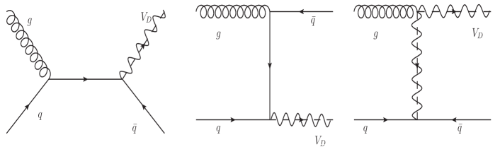
Figure 5: Feynman diagrams for the process $qg\rightarrow\bar{q}~{}V_{D}.$

The Feynman diagrams for this process are given in Fig 5. The total spin and color averaged amplitude-squared for the $qg$ initiated process in terms of Mandelstam variables is given by

$$\begin{multlined}\sum\overline{|\mathcal{M}_{qg}^{R}|^{2}}=\frac{g_{s}^{2}\lambda^{2}\mu^{4\epsilon}N_{D}(C_{D}su-C_{F}(s+u)^{2})}{2N_{C}(N_{C}^{2}-1)su(s+u)^{2}}\\ \times\Big{(}(n-2)(s^{2}+u^{2})+4t(u+s)+2(n-4)su+4t^{2}\Big{)}\end{multlined}\sum\overline{|\mathcal{M}_{qg}^{R}|^{2}}=\frac{g_{s}^{2}\lambda^{2}\mu^{4\epsilon}N_{D}(C_{D}su-C_{F}(s+u)^{2})}{2N_{C}(N_{C}^{2}-1)su(s+u)^{2}}\\ \times\Big{(}(n-2)(s^{2}+u^{2})+4t(u+s)+2(n-4)su+4t^{2}\Big{)}$$ (27)

Note that the spin average for the initial state gluon introduces a term dependent on the space-time dimension $n$ and also has a different color averaging factor compared to the $qq$ initiated process for real corrections. However, as expected the above expression does match with that for the $qq$ case without the spin and color averaging, under the interchange $t\leftrightarrow s$ and an overall sign. This is because of the crossing symmetry between $qq$ and $qg$ processes. The extra -ve sign in $qg$ case results when one fermion is moved from initial state to the final state.

The parton level cross section for the $qg$ initiated process is

$$\begin{multlined}\hat{\sigma}_{qg}^{R}=\frac{\hat{\sigma}_{0}}{\hat{s}}\frac{\alpha_{s}}{2\pi}C_{\epsilon}\Bigg{[}\Bigg{\{}\frac{-((1-\tau)^{2}+\tau^{2})}{2\epsilon_{\rm IR}}+\frac{3+2\tau-3\tau^{2}}{4}+((1-\tau)^{2}+\tau^{2}){\rm ln}(1-\tau)\Bigg{\}}\\ +\frac{C_{D}}{2C_{F}}\Bigg{\{}-1+\frac{2}{\tau}+\tau-2\tau^{2}+2(1+\tau){\rm ln}\tau\Bigg{\}}\Bigg{]},\end{multlined}\hat{\sigma}_{qg}^{R}=\frac{\hat{\sigma}_{0}}{\hat{s}}\frac{\alpha_{s}}{2\pi}C_{\epsilon}\Bigg{[}\Bigg{\{}\frac{-((1-\tau)^{2}+\tau^{2})}{2\epsilon_{\rm IR}}+\frac{3+2\tau-3\tau^{2}}{4}+((1-\tau)^{2}+\tau^{2}){\rm ln}(1-\tau)\Bigg{\}}\\ +\frac{C_{D}}{2C_{F}}\Bigg{\{}-1+\frac{2}{\tau}+\tau-2\tau^{2}+2(1+\tau){\rm ln}\tau\Bigg{\}}\Bigg{]},$$ (28)

where $\hat{\sigma}_{0}$ is given in Eq. 8. As shown above, the cross section has IR collinear divergence which we remove by factorization in $\overline{\rm MS}$ scheme. The required counter term is given by,

$$\sigma_{qg}^{\rm C.T.}=\frac{\hat{\sigma}_{0}}{\hat{s}}\frac{\alpha_{s}}{2\pi}\frac{(4\pi)^{\epsilon}}{\Gamma(1-\epsilon)}\Big{(}\frac{1}{\epsilon_{\rm IR}}+{\rm ln}\frac{\mu^{2}}{\mu_{F}^{2}}\Big{)}P_{qg}(\tau)$$ (29)

with $P_{qg}(\tau)=\frac{1}{2}\Big{[}(1-\tau)^{2}+\tau^{2}\Big{]}$. Hence the parton level cross section for the vector diquark production in $qg$ initiated channel is given by

$$\begin{multlined}\hat{\sigma}_{qg}=\hat{\sigma}_{qg}^{R}+\sigma_{qg}^{\rm C.T.}\\ =\frac{\hat{\sigma}_{0}}{\hat{s}}\frac{\alpha_{s}}{2\pi}\Bigg{[}P_{qg}(\tau)\Big{\{}{\rm ln}\Big{(}\frac{M_{D}^{2}}{\mu_{F}^{2}\tau}\Big{)}+2{\rm ln}(1-\tau)\Big{\}}+\frac{3+2\tau-3\tau^{2}}{4}\\ +\frac{C_{D}}{2C_{F}}\Big{\{}-1+\frac{2}{\tau}+\tau-2\tau^{2}+2(1+\tau){\rm ln}\tau\Big{\}}\Bigg{]}.\end{multlined}\hat{\sigma}_{qg}=\hat{\sigma}_{qg}^{R}+\sigma_{qg}^{\rm C.T.}\\ =\frac{\hat{\sigma}_{0}}{\hat{s}}\frac{\alpha_{s}}{2\pi}\Bigg{[}P_{qg}(\tau)\Big{\{}{\rm ln}\Big{(}\frac{M_{D}^{2}}{\mu_{F}^{2}\tau}\Big{)}+2{\rm ln}(1-\tau)\Big{\}}+\frac{3+2\tau-3\tau^{2}}{4}\\ +\frac{C_{D}}{2C_{F}}\Big{\{}-1+\frac{2}{\tau}+\tau-2\tau^{2}+2(1+\tau){\rm ln}\tau\Big{\}}\Bigg{]}.$$ (30)

The corresponding hadronic cross section is obtained by convoluting the above parton level cross section with the initial state quark and gluon distribution functions,

$$\sigma_{qg}=\int_{\tau_{0}}^{1}d\tau~{}\frac{\tau_{0}}{\tau^{2}}~{}\Big{[}(q\otimes g+g\otimes q)\Big{(}\frac{\tau_{0}}{\tau}\Big{)}\Big{]}~{}{\hat{\sigma}}_{qg}.$$ (31)

4 Decay Width: ${\cal O}(\alpha_{s})$ correction

Note that just like the LO cross sections for the production of the vector diquarks, the LO predictions for decay width of the particle also suffer from the renormalization scale uncertainties. Therefore for the sake of completion we would also like to estimate the effect of the QCD corrections on the decay width ($\Gamma$) of the vector diquark. Note that a primary requirement in assuming the narrow width approximation, one expects that the ratio $\Gamma/M_{D}$ is relatively small and not exceeding $\simeq 10\%$. In order to remain in that regime, it is necessary to check that the decay width does not change by much under higher-order corrections. In this section, we compute the NLO QCD corrections to the vector diquark decaying into a pair of light jets,

$$V_{D}(q)\rightarrow q_{i}(p_{1})+q_{j}(p_{2}).$$ (32)

The leading order total decay width is given by

$$\Gamma_{0}=\sum_{i}~{}{\lambda_{i}^{2}\over 24\pi}M_{D},$$ (33)

where $i$ is the number of light quark generations which can couple to the vector diquark of a given electric charge. We have assumed that we can neglect all quark masses in the decay products (including top quark). The virtual corrections to the decay width involve the same Feynman graphs shown in Fig. 2 and has the same singular structure as given in Eq. 18 for the on-shell vector diquark production. The same procedure followed in calculating the virtual corrections for the production cross section leads us to the UV renormalized virtual correction to the decay width which is given by

$$\Gamma^{V} = \Gamma_{0}\Bigg{[}1+{\alpha_{s}\over 2\pi}C_{\epsilon}\Bigg{\{}C_{F}\Bigg{(}-{2\over\epsilon_{IR}^{2}}-{3\over\epsilon_{IR}}-8+\pi^{2}\Bigg{)}$$ (34)

$$+C_{D}\Bigg{(}-{1\over\epsilon_{IR}}+{11\over 3}\ln\Big{(}{\mu_{R}^{2}\over M_{D}^{2}}\Big{)}+{77\over 18}-{2\pi^{2}\over 3}\Bigg{)}\Bigg{\}}\Bigg{]}.$$

However we must point out that the real gluon correction is inherently different from that of the production. To compute the real gluon correction to the decay width, we need to consider the following three body final state,

$$V_{D}(q)\rightarrow q_{i}(p_{1})+q_{j}(p_{2})+g.$$ (35)

Note that the calculation of real correction to diquark decay width requires three body phase space integration to be performed in $n=4-2\epsilon$ dimensions. For that we have followed the method given in Ref. Field . The final expression with the real correction to the decay width is then given by,

$$\Gamma^{R} = \Gamma_{0}{\alpha_{s}\over 2\pi}C_{\epsilon}\Bigg{[}C_{F}\Bigg{(}{2\over\epsilon_{IR}^{2}}+{3\over\epsilon_{IR}}+{19\over 2}-\pi^{2}\Bigg{)}+C_{D}\Bigg{(}{1\over\epsilon_{IR}}+{11\over 3}\Bigg{)}\Bigg{]}.$$ (36)

By adding the virtual and real corrections to decay width all the singularities cancel as expected by KLN theorem. Thus, the complete NLO QCD correction to the diquark decay width is given by (from Eq. 34 and Eq. 36),

$$\Gamma_{\rm NLO}=\Gamma_{0}\Bigg{[}1+{\alpha_{s}\over 2\pi}\Bigg{\{}{3\over 2}C_{F}+C_{D}\Bigg{(}{143\over 18}-{2\pi^{2}\over 3}+{11\over 3}\ln\Big{(}{\mu_{R}^{2}\over M_{D}^{2}}\Big{)}\Bigg{)}\Bigg{\}}\Bigg{]}.$$ (37)

The corresponding expression for the case of scalar diquark is given in Appendix D. From Eq. 37, we observe that the coefficient of $C_{F}$ is similar to that in SM (NLO QCD correction of an electroweak vector boson decaying into quark-antiquark pair) although here the final state is a quark-quark pair. We also find that a non-trivial contribution to the NLO decay width arises from the other Casimir, $C_{D}$ which takes different values for the two color representations of the vector diquark.

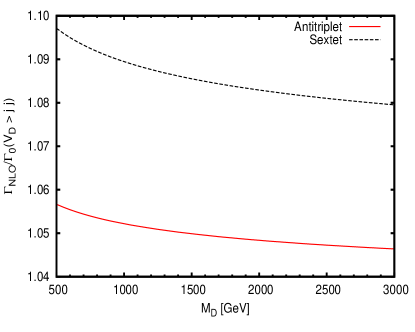
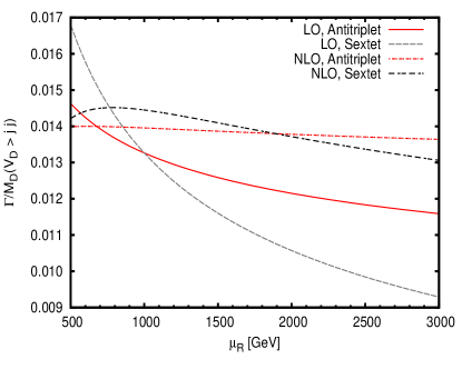
Figure 6: Dependence of decay width on $M_{D}$ (left) and on renormalization scale $\mu_{R}$ (right) to ${\cal O}(\alpha_{s})$. To show the $\mu_{R}$ dependence we chose $\lambda(M_{D})=1$ where $M_{D}=1$ TeV.

We calculate the relevant $K$-factor defined as the ratio of the NLO width to that of the LO width and plot it in Fig. 6. In the left panel of Fig. 6, we have shown the dependence of the NLO $K-$factor for the decay width on the diquark mass. As $\mu_{R}=M_{D}$ we can clearly see that the logarithmic term in Eq. 37 will not contribute and we should expect a constant value for a particular diquark representation. We however observe a slight variation for the NLO $K$-factor for the widths of the antitriplet and sextet vector diquarks as we vary the mass $M_{D}$, which is only arising because of the running of the strong coupling $\alpha_{s}$ (we have taken $\alpha_{s}(M_{Z})=0.1184$ as the reference value). We find that $K$-factor for the sextet case is larger than the antitriplet due to larger $C_{D}$ and increases the LO width by about $8-10\%$ for the mass range $M_{D}=0.5-3$ TeV. The corresponding LO width for the antitriplet vector diquark is modified less and increases by about $4.5-6\%$ with the $K$-factor. On the right panel of Fig. 6, we show the scale dependence $\mu_{R}$ of the decay width at LO and NLO and for sextet and antitriplet vector diquark states. As a reference point, we have chosen $\lambda(M_{D})=1$ where $M_{D}=1$ TeV and we vary $\mu_{R}$ between $M_{D}/2$ to $3M_{D}$. The LO scale dependence is entirely due to the running of the coupling (see Fig. 3). We can clearly see that the inclusion of ${\cal O}(\alpha_{s})$ correction has significantly reduced the scale dependence. As one would expect, due to the smaller color factor $C_{D}$ the scale variation for the antitriplet case is also smaller as compared to the scale variation for the sextet case.

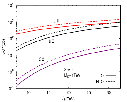
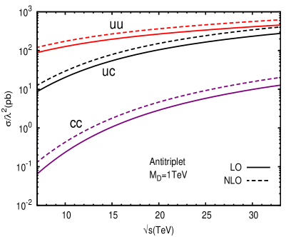
Figure 7: Vector diquark production cross sections for the sextet and antitriplet cases at LO and NLO through the $uu,~{}uc$ and $cc$ initial states as a function of the $pp$ hadronic center of mass energy.

5 Numerical Analysis and Results

In this section, we discuss the LO and NLO results for the vector diquark production at the LHC. We have used the CTEQ6L1 (CTEQ6M) Pumplin:2002vw PDF’s for the parton fluxes in the colliding protons for our LO (NLO) results. In our calculations we choose $\mu_{F}=\mu_{R}=M_{D}$ as the central scale for factorization and renormalization unless otherwise stated. Using our analytic results for the vector diquark production derived in the previous section we can now study how the cross sections are affected as a function of the collider center of mass energy ($\sqrt{s}$) as well as for different values of the mass ($M_{D}$) of the vector diquark. The LHC has already completed its run at two different $\sqrt{s}$ of $7$ and $8$ TeV and there are plans of running the machine at $13$ and $14$ TeV while future upgrades to $33$ TeV is also possible. In Fig. 7 we show the LO and NLO hadronic cross sections for the on-shell vector diquark production as a function of the proton-proton collider center of mass energy, for a fixed value of $M_{D}=1$ TeV. Note that the variation observed in the LO cross section can be attributed to the initial parton PDF’s only where, as the center of mass energy rises the on-shell condition of the diquark production for $M_{D}=1$ TeV forces the colliding partons to carry a much smaller $x$ (momentum fraction) of the proton beam energy. Therefore the initial quark’s flux grows giving rise to increase in the production cross section. The variation of the NLO cross section is however governed by both the partonic cross section and the PDF’s although the feature attributed to the LO behavior due to the PDF’s is similar. The plot is shown for three different quark-quark initial states, namely $uu,cc$ and $uc$.

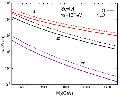
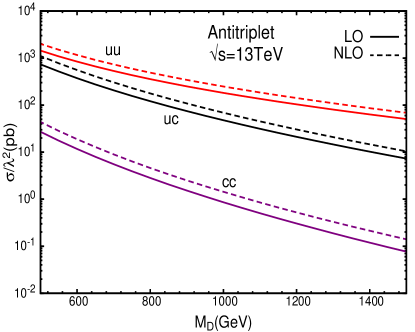
Figure 8: Production cross section of the sextet and antitriplet vector diquarks at LO and NLO through the $uu,~{}uc$ and $cc$ initial states as a function of the diquark mass $M_{D}$ at LHC with $\sqrt{s}=13$ TeV.

It is worth recalling the fact that the coupling of the vector diquark can be generation and flavor dependent. Therefore one can consider the diquark to be produced through initial partons of a particular fermion generation and flavor or it can be produced, mediated by interactions between different generations. We have chosen to normalize the cross sections with the coupling strength $\lambda$ squared so that it does not play a role here. Also note that although we always choose $\lambda(M_{D})=1$ we have neglected the effect of the running of the coupling constant $\lambda$ in Fig. 7. Quite clearly, cross sections for the valence quark initiated processes are significantly large and reach appreciably high rates of above $\sim 100$ picobarns (pb) for ${\mathcal{O}(1)}$ coupling strengths. Even the sea quark rates rise from a few $100$ femtobarns (fb) to few ten’s of picobarns for both the sextet and antitriplet vector diquarks for ${\mathcal{O}(1)}$ coupling strengths. When compared with the scalar diquark production rates we note that the LO cross section for the vector diquark production is exactly twice that of the scalar diquark. Again, as against the scalar case where same flavor initial states are disallowed for the antitriplet case because of the antisymmetric property of the $K_{ab}$, one gets all modes contributing in the vector case Han:2010rf . Thus a vector diquark which transforms as an antitriplet under $SU(3)_{C}$ would be produced through the initial valence $uu$ and $dd$ states resulting in a much higher cross section for the dijet final state compared to the scalar diquark which would have dominant production mode through $ud$ initial states. One important point to note here is that if only flavor diagonal couplings are allowed for the $uu$ type interactions then the vector antitriplet diquark will mediate same-sign top pair productions while the scalar diquarks will not, which would be a very interesting signal at the LHC.

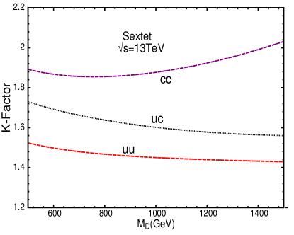
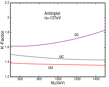
Figure 9: Illustrating the NLO $K$-factors for the production of both sextet and antitriplet vector diquark at the LHC with $\sqrt{s}=13$ TeV, through the initial states $uu,~{}uc$ and $cc$ as a function of the vector diquark mass $M_{D}$.

Since the vector diquark mass ($M_{D}$) is a free parameter, it is also instructive to know how the production cross section varies as a function of the diquark mass. We plot both the LO and NLO cross sections as a function of $M_{D}$ at the LHC run with $\sqrt{s}=13$ TeV in Fig. 8. The plot is again shown for three different initial state combinations of quarks, namely $uu,cc$ and $uc$. All these would lead to the production of a vector diquark of charge +4/3. The coupling strength has been factored out as before. We have varied $M_{D}$ in the range between $500$ GeV to $1.5$ TeV. Due to phase space suppression, the cross section goes down as we increase $M_{D}$. It is worth pointing it out here that due to the difference in $N_{D}$, the sextet diquark production cross section at LO is just twice that of the antitriplet production cross section (see Eq. 8). However, the NLO cross sections are markedly different for the two cases and therefore the NLO cross sections for the sextet are no longer twice that of the antitriplet production. This will be evident from the $K$-factor estimates which we show next. Note that as all the different charged vector diquark productions are driven by the same color algebra for a given representation of $SU(3)_{C}$ the cross sections for them are eventually driven by the initial quark PDF’s that participate in the production. Therefore the nature of the plots for the production cross section for the $|Q|=2/3,1/3$ charged diquarks is very similar.

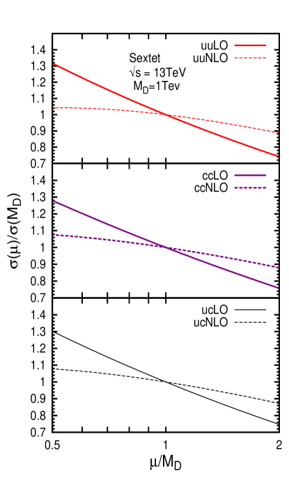
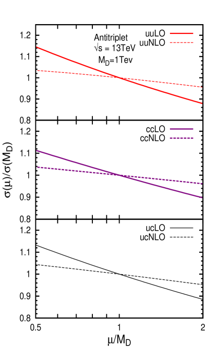
Figure 10: Showing the scale dependence of LO and NLO production cross sections for sextet and antitriplet diquark states of mass $M_{D}=1$ TeV at the LHC with $\sqrt{s}=13$ TeV .

In Fig. 9 we show the dependence of NLO $K$-factor, defined as the ratio of the NLO cross section to the LO cross section, on the vector diquark mass $M_{D}$ for both sextet and antitriplet diquark states. The $K$-factors for the $uu$ and $dd$ initiated production are between 1.5 and 1.3 for the mass range considered. We observe that the $K$-factor for $uu$ and $uc$ initial states decrease with $M_{D}$ while for $cc$ initial state it increases which is mainly because of the difference in the PDF distributions for the valence and sea quarks in the proton. Also note that the $K$-factors in the case of the vector sextet diquark are larger compared to their corresponding values in the vector triplet case which is unlike that observed for the scalar diquarks. For the scalar diquarks there is a partial cancellation between the $C_{F}$ and $C_{D}$ terms, which gives a smaller $K$-factor for the sextet case compared to the antitriplet Han:2009ya , while the $C_{F}$ and $C_{D}$ terms in the vector case come with the same sign. However other features such as a larger $K$-factor for the sea quarks compared to the valence quarks remains the same, as this comes from their PDF behaviour as the factorization scale varies.

		$\sqrt{s}=8~{}{\rm TeV}$
		$M_{D}=1~{}{\rm TeV}$			$M_{D}=3~{}{\rm TeV}$
qq	State	LO	NLO	$K_{F}$	LO	NLO	$K_{F}$
	S	$212^{+34.6}_{-27.3}$	$306^{+4.5}_{-12.1}$	1.4	$1.08^{+41.8}_{-30.3}$	$1.47^{+10.4}_{-15.9}$	1.3
$uu$	AT	$106^{+17.2}_{-13.9}$	$144^{+3.9}_{-5.2}$	1.3	$0.54^{+25.2}_{-19.16}$	$0.69^{+7.7}_{-8.9}$	1.2
	S	$227^{+35.6}_{-27.8}$	$334^{+5.2}_{-12.7}$	1.4	$0.67^{+43.1}_{-30.9}$	$0.92^{+11.3}_{-16.5}$	1.3
$ud$	AT	$113^{+18.0}_{-14.5}$	$157^{+4.3}_{-5.6}$	1.3	$0.33^{+26.4}_{-19.84}$	$0.43^{+8.3}_{-9.5}$	1.2
	S	$57.3^{+36.6}_{-28.3}$	$86.0^{+5.8}_{-13.2}$	1.4	$0.09^{+44.5}_{-31.4}$	$0.13^{+12.3}_{-17.1}$	1.3
$dd$	AT	$28.6^{+18.8}_{-15.1}$	$40.4^{+4.7}_{-6.0}$	1.4	$0.04^{+27.5}_{-20.5}$	$0.06^{+8.9}_{-10.0}$	1.2
	S	$0.89^{+36.6}_{-28.4}$	$1.40^{+8.3}_{-14.0}$	1.5	${5.46\times 10^{-5}}^{+45.1}_{-31.7}$	${1.38\times 10^{-4}}^{+12.2}_{-16.8}$	2.5
$ss$	AT	$0.44^{+18.9}_{-15.2}$	$0.64^{+5.3}_{-6.1}$	1.4	${2.73\times 10^{-5}}^{+28.1}_{-20.8}$	${6.39\times 10^{-5}}^{+8.4}_{-9.4}$	2.3
	S	$0.95^{+34.2}_{-27.3}$	$1.70^{+8.0}_{-13.4}$	1.7	${4.33\times 10^{-5}}^{+41.6}_{-30.2}$	${1.92\times 10^{-4}}^{+11.1}_{-16.0}$	4.4
$sc$	AT	$0.47^{+16.8}_{-14.0}$	$0.77^{+4.7}_{-5.3}$	1.6	${2.16\times 10^{-5}}^{+25.0}_{-19.1}$	${8.87\times 10^{-5}}^{+7.5}_{-8.7}$	4.1
	S	$0.24^{+31.7}_{-26.2}$	$0.51^{+7.6}_{-12.7}$	2.1	${8.65\times 10^{-6}}^{+38.2}_{-28.7}$	${6.55\times 10^{-5}}^{+10.0}_{-15.1}$	7.5
$cc$	AT	$0.12^{+14.6}_{-12.6}$	$0.23^{+4.1}_{-4.6}$	1.9	${4.32\times 10^{-6}}^{+22.0}_{-17.3}$	${3.01\times 10^{-5}}^{+6.6}_{-7.8}$	6.9
	S	${0.09}^{+24.1}_{-22.5}$	$0.19^{+6.0}_{-10.3}$	2.0	${3.31\times 10^{-6}}^{+31.3}_{-25.6}$	${1.81\times 10^{-5}}^{+6.7}_{-12.4}$	5.4
$bb$	AT	${0.04}^{+8.0}_{-8.3}$	${0.08}^{+2.1}_{-2.0}$	1.7	${1.65\times 10^{-6}}^{+15.9}_{-13.7}$	${8.24\times 10^{-6}}^{+3.6}_{-5.0}$	4.9

Table 1: The LO and NLO cross sections (in pb) and K-factors for vector diquark production via different initial quark states at $\sqrt{s}=8$ TeV. We give the cross sections for both the sextet (S) and antitriplet (AT) diquarks. The uncertainties (in $\%$) given for the cross sections are due to the the choice of scale $Q=\mu$ and is obtained by varying the scale from $M_{D}/2$ to $2M_{D}$. We choose two reference values of the vector diquark mass $M_{D}=1,3$ TeV and a fixed value for the coupling, $\lambda=1$.

One of the primary reasons for calculating the higher-order corrections to a scattering process is to minimize the scale dependence on measurable observables such as cross sections, that would affect the event rate estimates at experiments. We therefore make an estimate of the dependence of the choice of scale on the LO and NLO cross sections for the vector diquark production. To illustrate this we vary both the renormalization $\mu_{R}$ and factorization $\mu_{F}$ scale by a factor of two about the central scale $\mu=M_{D}$ keeping $\mu_{R}=\mu_{F}=\mu$ throughout. Note that the renormalization scale dependence of the leading order cross section is governed by the one-loop running of the coupling parameter $\lambda$. Thus the scale dependence of the LO cross section has an uncertainty of ${\cal O}(\alpha_{s})$. Although, while predicting the scale dependence of NLO cross section, we should use two-loop running of the coupling, leading to an uncertainty of ${\cal O}(\alpha_{s}^{2})$: in absence of the two-loop result for running coupling we use Eq. 20 for predicting the renormalization scale dependence for both the LO and NLO cross sections for the vector diquark production at LHC with $\sqrt{s}=13$ TeV. We plot our results in Fig. 10, where we can see clearly how the scale dependence of the NLO cross section is significantly reduced compared to the LO cross section. While the LO cross section varies between $\sim\pm 30\%$ for the vector sextet diquark for the three initial states $uu,~{}uc$ and $cc$ as $\mu$ varies between $M_{D}/2$ to $2M_{D}$, the dependence is reduced to $\sim\pm 10\%$ for the NLO cross sections. For the antitriplet vector diquark, the dependence is relatively less compared to the sextet, of about $\sim\pm(12-14)\%$ for the LO cross sections which gets reduced to $\sim\pm 4\%$ for the NLO result. Notice that the scale uncertainty in antitriplet case is much smaller than that in sextet case which is reduced further when the NLO results are included. This is because of the $C_{D}$ dependence (see Eq. 20 and Eq. 25) which is smaller for the antitriplet ($C_{D}=4/3$) compared to the sextet ($C_{D}=10/3$).

		$\sqrt{s}=13~{}{\rm TeV}$
		$M_{D}=1~{}{\rm TeV}$			$M_{D}=3~{}{\rm TeV}$
qq	State	LO	NLO	$K_{F}$	LO	NLO	$K_{F}$
	S	$364^{+31.6}_{-25.8}$	$528^{+4.2}_{-11.3}$	1.4	$6.91^{+35.5}_{-27.3}$	$9.60^{+6.1}_{-12.5}$	1.3
$uu$	AT	$182^{+14.6}_{-12.1}$	$249^{+3.4}_{-4.4}$	1.3	$3.45^{+19.7}_{-15.6}$	$4.54^{+4.8}_{-6.2}$	1.3
	S	$443^{+32.3}_{-26.2}$	$660^{+4.7}_{-11.7}$	1.4	$5.79^{+36.6}_{-27.8}$	$8.12^{+6.8}_{-13.1}$	1.4
$ud$	AT	$221^{+15.1}_{-12.6}$	$310^{+3.7}_{-4.7}$	1.3	$2.89^{+20.6}_{-16.2}$	$3.83^{+5.2}_{-6.7}$	1.3
	S	$126^{+33.0}_{-26.5}$	$192^{+5.2}_{-12.1}$	1.5	$1.15^{+37.6}_{-28.3}$	$1.62^{+7.5}_{-13.7}$	1.4
$dd$	AT	$63.3^{+15.}_{-13.0}$	$90.2^{+3.9}_{-4.9}$	1.4	$0.57^{+21.5}_{-16.8}$	$0.76^{+5.7}_{-7.1}$	1.3
	S	$4.75^{+32.1}_{-26.2}$	$7.50^{+7.6}_{-12.9}$	1.5	${3.73\times 10^{-3}}^{+38.8}_{-28.9}$	${6.43\times 10^{-3}}^{+8.9}_{-14.1}$	1.7
$ss$	AT	$2.37^{+14.9}_{-12.6}$	$3.39^{+4.4}_{-4.9}$	1.4	${1.86\times 10^{-3}}^{+22.6}_{-17.5}$	${2.97\times 10^{-3}}^{+6.1}_{-7.1}$	1.6
	S	$5.82^{+30.1}_{-25.3}$	$9.91^{+7.7}_{-12.5}$	1.7	${3.31\times 10^{-3}}^{+36.4}_{-27.8}$	${7.81\times 10^{-3}}^{+8.1}_{-13.3}$	2.3
$sc$	AT	$2.91^{+13.2}_{-11.5}$	$4.44^{+4.1}_{-4.4}$	1.5	${1.65\times 10^{-3}}^{+20.4}_{-16.2}$	${3.60\times 10^{-3}}^{+5.3}_{-6.3}$	2.1
	S	$1.72^{+27.9}_{-24.2}$	$3.23^{+7.6}_{-12.0}$	1.8	${7.26\times 10^{-4}}^{+33.9}_{-26.6}$	${2.37\times 10^{-3}}^{+7.3}_{-12.5}$	3.2
$cc$	AT	$0.86^{+11.3}_{-10.2}$	$1.43^{+3.7}_{-3.8}$	1.6	${3.63\times 10^{-4}}^{+18.2}_{-14.9}$	${1.09\times 10^{-3}}^{+4.6}_{-5.6}$	3.0
	S	$0.73^{+20.8}_{-20.6}$	$1.34^{+6.8}_{-10.2}$	1.8	${2.80\times 10^{-4}}^{+27.9}_{-23.7}$	${8.16\times 10^{-4}}^{+5.3}_{-10.3}$	2.9
$bb$	AT	$0.36^{+5.1}_{-6.0}$	$0.58^{+2.1}_{-1.7}$	1.5	${1.40\times 10^{-4}}^{+12.9}_{-11.5}$	${3.68\times 10^{-4}}^{+2.6}_{-3.3}$	2.6

Table 2: The LO and NLO cross sections (in pb) and K-factors for vector diquark production via different initial quark states at $\sqrt{s}=13$ TeV. All other choices are similar to that in Table 1.

Note that we have till now chosen to illustrate our results with figures for only the 4/3 charged diquark production that couple to the first two generations of the fermions. But we should also note here that the vector diquarks with the 2/3 and 1/3 charge can have substantial rates only affected by the initial PDF’s of the contributing quarks. So to put the rate of production for the different vector diquarks in perspective we calculated all the modes that could contribute to its production and present the LO and NLO cross sections in the relevant channels with scale uncertainties at $\sqrt{s}=8$ and $\sqrt{s}=13$ TeV run of LHC. To highlight the cross sections we have chosen two representative values of diquark mass $M_{D}=1$ and $3$ TeV and fixed the coupling $\lambda=1$. We show the cross sections for LHC with $\sqrt{s}=8$ TeV and $13$ TeV in Table 1 and Table 2 respectively. We assume that the couplings of vector diquarks mediating quarks of different generations is suppressed. So out of the 15 possible combinations we only consider 7 combinations with no inter-generation vertices. One can clearly see that the valence quark contributions dominate, with the $uu$ and $dd$ contributions being a few orders of magnitude higher than $cc$ and $ss$ respectively for $M_{D}=1$ TeV in Table 1. For the 3 TeV diquark, the difference in orders is nearly doubled. A similar behavior is seen in Table 2. It is quite easy to understand that this happens due to the PDF’s of the quarks in consideration and the momentum fraction $x$ of the initial proton that they carry. However the notable thing to consider is the fact that due to

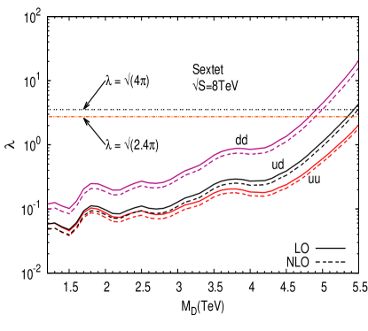
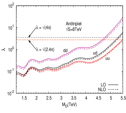
Figure 11: The constraints on the mass $M_{D}$ and coupling $\lambda$ at $95\%$ C.L. for the sextet and antitriplet vector diquark states at the LHC with $\sqrt{s}=8$ TeV using the LO and NLO cross sections. The values $\sqrt{4\pi}$ represents the perturbative limit for $\lambda$ while $\lambda=\sqrt{2.4\pi}$ gives the upper bound on the coupling for $\Gamma/M_{D}<10\%$.

quite small production cross sections for the diquarks produced through second generation quarks, even with order 1 coupling, the mass limits on them would be considerably weaker compared to the diquarks coupling to the first generation. As we have already determined a rough order of magnitude by which the cross sections differ for the first and second generation vector diquarks, it would give us a comparative idea of the limits on their coupling and mass from that derived for any one generation. We already have updated limits from dijet data by both ATLAS and CMS collaborations at the LHC Aad:2014bc ; Khachatryan:2015jd . We use Ref. Khachatryan:2015jd of the CMS collaboration to derive the limits on the vector diquark mass and coupling. The CMS collaboration has given the upper bound on the cross sections for different resonant mass values which can be compared with the parton-level resonant production cross section $(\sigma)$ times branching fraction $({\mathcal{B}})$ in the narrow-width approximation using $\sigma\mathcal{BA}$, where ${\mathcal{A}}$ is an acceptance factor $\sim 0.6$ Khachatryan:2015jd . We use this to derive limits for the vector diquark (both sextet and antitriplet) mass $M_{D}$ and its coupling $\lambda$ which interacts only with the first generation quarks. As these would be contributions coming through the valence quarks with the largest rates, the limits on the diquark coupling to the second and third generation quarks would be much weaker. In Fig. 11 we show the $95\%$ C.L. constraints on the mass and couplings of the vector diquark produced through $uu,ud$ and $dd$ fusion using the dijet data from Ref. Khachatryan:2015jd . The plots illustrate that all values of $M_{D}$ and $\lambda$ which are above the curves are ruled out by the CMS dijet data at $95\%$ C.L.. Note that we assume that the vector diquark couples to only one pair of quarks. We also show the perturbative limit of $\lambda=\sqrt{4\pi}$ in the plots, while $\lambda=\sqrt{2.4\pi}$ gives the upper bound on the coupling for $\Gamma/M_{D}<10\%$. As expected the strongest limits are for the $4/3$ charged diquark which couples to $uu$. The NLO corrections do modify the constraints to give slightly stronger limits compared to the LO results. For example, given a fixed value of the coupling $\lambda=0.5$ we find the $dd$ initiated LO result for the antitriplet vector diquark gives a lower bound of $M_{D}\simeq 3.03$ TeV whereas the NLO corrections improve the limit by about 100 GeV to $M_{D}\simeq 3.12$ TeV. The corresponding limits for the sextet vector diquark at LO ($M_{D}\simeq 3.32$ TeV) changes to $M_{D}\simeq 3.42$ TeV at NLO. The corrections in the other modes are also found to be between $\sim$ 50-100 GeV. We have chosen not to show the effect of the associated scale uncertainties on the limits obtained. It should suffice to mention that the bounds using the LO cross sections would incorporate a much larger uncertainty band in the constraints compared to the NLO which is evident from the details given in Table 1 and Table 2. Also note that as the cross section for the second generation induced productions are at least 2 or more orders of magnitude smaller for similar couplings, the limits on the couplings would be relaxed by a factor of $10$ or larger, allowing larger couplings for similar diquark mass. However one clearly finds a large parameter region still allowed for vector diquarks which should be explored at the upcoming run of LHC with $\sqrt{s}=13$ TeV.

6 Summary

In this work we have calculated the NLO QCD corrections to the vector diquark production at hadron colliders, namely the LHC. As colored particles are surely to be produced with large cross sections at hadron colliders, the discovery of any such state could be the first step towards discovering BSM physics at the LHC. Colored particles such as the vector diquark can mediate larger production rates for dijet and multijet events. We show how the NLO corrections to the vector diquark production affects the cross sections for the sextet and antitriplet representations. As the vector diquark couplings to the quark pair can be generation dependent, we find that valence quark processes have $K$-factors in the range of 1.5 to 1.3 for a mass range of 0.5-1.5 TeV which decrease as we go higher in mass. The $sea$ quark initiated production modes are found to have increasing values of the $K$-factor as the diquark mass is increased. We also find that unlike the scalar diquarks, the sextet vector diquark has larger NLO corrections compared to the antitriplet. We also illustrate the scale uncertainties in the cross section for both the sextet and antitriplet vector diquarks and find that the sextet vector diquark exhibits bigger scale uncertainty at LO compared to the antitriplet. The NLO corrected cross sections for both cases are found to show much lesser dependence on the scale variation. We also calculate the NLO corrections to the width of the vector diquark decaying to a pair of quarks. As a narrow-width approximation is considered large corrections to the width can affect predictions for relevant final states. We find that the $K$-factor for decay width of the sextet diquark is around $1.08-1.1$ while it is around $1.05$ for the antitriplet which is relatively smaller than that for the production cross section. However the scale uncertainties are relatively large for the decay width which get reduced by taking the NLO corrected widths.

We have calculated cross sections for the vector diquark production at LHC with $\sqrt{s}=8$ and $13$ TeV arising from different generation quarks. We use the dijet data from the CMS collaboration for LHC with $\sqrt{s}=8$ TeV to put limits on the vector diquark mass and its coupling. We find that a large parameter region is still allowed for vector diquarks which should be explored at the upcoming run of LHC at $\sqrt{s}=13$ TeV. The current limits by the LHC experiments on the resonant particles include scalar diquarks but do not include vector diquarks. We have shown that using the same data one could also search for the vector diquarks and give search limits for such particles.

Appendix A Feynman rules

The interaction Lagrangians given in Eqns 1 and 2 give the following Feynman rules (all momenta incoming) :

• ${\bf\bar{q^{c}_{a}}(p_{1})q_{b}^{\prime}(p_{2})V_{i}^{\mu}(p_{3}):}$             $\frac{i\lambda_{qq^{\prime}}}{\sqrt{1+\delta_{qq^{\prime}}}}\gamma_{\mu}(K^{i}_{ab}P_{\tau}-\delta_{qq^{\prime}}K^{i}_{ba}P_{\tau^{\prime}})$
  where $P_{\tau}(P_{\tau^{\prime}})$ can be $P_{L/R}(P_{R/L})$.

• ${\bf V_{i}^{\mu_{1}}(p_{1})V_{j}^{*\mu_{2}}(p_{2})G^{A,\mu_{3}}(p_{3}):}$    $-ig_{s}T^{A}_{ji}[g^{\mu_{1}\mu_{2}}(p_{1}-p_{2})^{\mu_{3}}+g^{\mu_{2}\mu_{3}}(p_{2}-p_{3})^{\mu_{1}}\\ \hskip 274.6262pt+g^{\mu_{3}\mu_{1}}(p_{3}-p_{1})^{\mu_{2}}]$

Appendix B One-loop scalars

Here we list various tadpole ($A_{0}$), bubble ($B_{0}$) and triangle ($C_{0}$) scalar integrals required in the calculation of virtual corrections in sections 3 and 4. For simplicity we take out the universal one-loop factor from these integrals which arise in DR and use the following notation,

$$I_{0}=\frac{i}{16\pi^{2}}\frac{(4\pi\mu^{2})^{\epsilon}}{\Gamma(1-\epsilon)}~{}\tilde{I}_{0}.$$ (38)

We have labeled the UV and IR singularities of scalar integrals explicitly in our calculations. In DR, $\epsilon_{\rm UV}=\epsilon_{\rm IR}=\epsilon$.

$$\tilde{A}_{0}(m^{2}) =(m^{2})^{(1-\epsilon)}\Big{[}\frac{1}{\epsilon_{\rm UV}}+1\Big{]}$$ (39)

$$\tilde{B}_{0}(s;0,0) =\frac{1}{(-s)^{\epsilon}}\Big{[}\frac{1}{\epsilon_{\rm UV}}+2\Big{]}$$ (40)

$$\tilde{B}_{0}(0;0,m^{2}) =\frac{1}{(m^{2})^{\epsilon}}\Big{[}\frac{1}{\epsilon_{\rm UV}}+1\Big{]}$$ (41)

$$\tilde{B}_{0}(0;0,0) =\frac{1}{(\mu^{2})^{\epsilon}}\Big{[}\frac{1}{\epsilon_{\rm UV}}-\frac{1}{\epsilon_{\rm IR}}\Big{]}$$ (42)

$$\tilde{B}_{0}(m^{2};0,m^{2}) =\frac{1}{(m^{2})^{\epsilon}}\Big{[}\frac{1}{\epsilon_{\rm UV}}+2\Big{]}$$ (43)

$$\frac{\partial}{\partial s}\tilde{B}_{0}(s;0,m^{2})|_{s=m^{2}} =(m^{2})^{(-1-\epsilon)}\Big{[}-\frac{1}{2\epsilon_{\rm IR}}-1\Big{]}$$ (44)

$$\tilde{C}_{0}(0,0,s;0,0,0) =\frac{1}{(-s)^{\epsilon}}\Big{[}\frac{1}{s}\Big{(}\frac{1}{\epsilon_{\rm IR}^{2}}\Big{)}\Big{]}$$ (45)

$$\tilde{C}_{0}(0,0,m^{2};0,0,m^{2}) =(m^{2})^{(-1-\epsilon)}\Big{[}-\frac{1}{2\epsilon_{\rm IR}^{2}}-\frac{\pi^{2}}{12}\Big{]}$$ (46)

The derivative of bubble function in Eq. 44 is used in the calculation of $Z_{2}^{q}$ and $Z_{2}^{D}$.

Appendix C Plus function

For a function $f(x)$, singular at $x=1$, and a smooth function $g(x)$, the plus function is defined by the following relation,

$$\int_{0}^{1}dxf_{+}(x)g(x)=\int_{0}^{1}f(x)[g(x)-g(1)].$$ (47)

Few plus function related identities which have been very useful in the calculation of real corrections are,

$$\int_{a}^{1}dxf_{+}(x)g(x) = \int_{a}^{1}dxf(x)[g(x)-g(1)]-g(1)\int_{0}^{a}dxf(x)$$ (48)

$$\frac{1}{(1-\tau)^{(1+2\epsilon)}} = \frac{1}{(1-\tau)_{+}}-2\epsilon\Big{[}\frac{\ln(1-\tau)}{1-\tau}\Big{]}_{+}-\frac{1}{2\epsilon}\delta(1-\tau)$$ (49)

$$\frac{f(x)}{(1-\tau)_{+}} = \Big{[}\frac{f(x)}{(1-\tau)}\Big{]}_{+}+\delta(1-\tau)\int_{0}^{1}dz~{}\frac{f(z)-f(1)}{1-z}$$ (50)

Appendix D ${\cal O}(\alpha_{s})$ Correction to scalar diquark decay width

The NLO QCD correction to the decay width for scalar diquark decaying into a pair of light jets is given by,

$$\Gamma_{\rm NLO}=\Gamma_{0}\Big{\{}1+\frac{\alpha_{s}}{2\pi}\Big{[}C_{D}\Big{(}\frac{5}{2}-\frac{2}{3}\pi^{2}\Big{)}+C_{F}\Big{(}3~{}{\rm ln}\Big{(}\frac{\mu_{R}^{2}}{M_{D}^{2}}\Big{)}+\frac{17}{2}\Big{)}\Big{]}\Big{\}},$$ (51)

where, the LO decay width $\Gamma_{0}$, is given by

$$\Gamma_{0}=\frac{\lambda^{2}}{16\pi}~{}M_{D}.$$ (52)

Note that the $C_{F}$ part is exactly the same as one gets in the NLO QCD calculation of $H\to b{\bar{b}}$ decay width Braaten:1980xx . We have used the following interaction Lagrangian for the scalar diquark ($\Phi_{i}$) case,

$${\cal L}^{\phi}=\frac{\lambda}{(1+\delta_{qq^{\prime}})}\;[\Phi_{i}\bar{q^{c}_{a}}K^{i}_{ab}P_{\tau}q^{\prime}_{b}+{\rm h.c.}]+(D_{\mu}\Phi_{i})^{\dagger}(D^{\mu}\Phi_{i})-M_{D}^{2}\Phi_{i}^{\dagger}\Phi_{i}.$$ (53)

It should be noted that the coupling of the scalar diquark with two same flavor quarks is zero in antitriplet case.

Appendix E Useful relations

Some of the relations among color factors that we have used to simplify various expressions in sections 3 and 4, are given below. For a more complete list one may refer to Ref. Han:2009ya .

$$t^{A}_{ab}t_{A,bc} = C_{F}\delta_{ac}$$ (54)

$$T^{A}_{ij}T_{A,jk} = C_{D}\delta_{ik}$$ (55)

$${\rm Tr}(K^{i}{\bar{K}}^{i}) = N_{D}$$ (56)

$${\rm Tr}(K^{i}t^{A}t_{A}{\bar{K}}^{i}) = C_{F}N_{D}$$ (57)

$${\rm Tr}(K^{i}t^{A}{\bar{K}}^{i}(t_{A})^{T}) = \pm\frac{1}{2}C_{F}N_{C}$$ (58)

$$T^{A}_{ij}{\rm Tr}(K^{j}t^{A}{\bar{K}}^{i}) = T^{A}_{ij}{\rm Tr}({\bar{K}}^{i}(t^{A})^{T}K^{j})=\frac{1}{2}C_{D}N_{D}$$ (59)

$$\pm C_{F}N_{C} = -2C_{F}N_{D}+C_{D}N_{D}.$$ (60)

In the above $t^{A}_{ab}$ are the $SU(3)_{C}$ generators in fundamental representation while $T^{A}_{ij}$ are the generators in the diquark representation of $SU(3)_{C}$.

To calculate the real corrections to the 2-body decay of the diquark, the following relation has been used in simplifying the three body phase space integration in $n=4-2\epsilon$ dimensions.

$$\Gamma(2z)=\frac{2^{2z-1}}{\sqrt{\pi}}\Gamma(z)\Gamma\Big{(}z+\frac{1}{2}\Big{)}.$$ (61)

References

- (1) G. Aad et al. [ATLAS Collaboration], Phys. Lett. B 716 (2012) 1 [arXiv:1207.7214 [hep-ex]].
- (2) S. Chatrchyan et al. [CMS Collaboration], Phys. Lett. B 716 (2012) 30 [arXiv:1207.7235 [hep-ex]].
- (3) R. Barbier et al., Phys. Rept. 420, 1 (2005) [arXiv:hep-ph/0406039].
- (4) J. L. Hewett and T. G. Rizzo, Phys. Rept. 183, 193 (1989).
- (5) S. Chakdar, T. Li, S. Nandi and S. K. Rai, Phys. Rev. D 87, no. 9, 096002 (2013) [arXiv:1302.6942 [hep-ph]].
- (6) S. Chakdar, T. Li, S. Nandi and S. K. Rai, Phys. Lett. B 718, 121 (2012) [arXiv:1206.0409 [hep-ph]].
- (7) T. Li, Z. Murdock, S. Nandi and S. K. Rai, Phys. Rev. D 85, 076010 (2012) [arXiv:1201.5616 [hep-ph]].
- (8) P. H. Frampton and S. L. Glashow, Phys. Lett. B 190, 157 (1987).
- (9) J. Bagger, C. Schmidt and S. King, Phys. Rev. D 37, 1188 (1988).
- (10) C. T. Hill, Phys. Lett. B 266, 419 (1991).
- (11) C. T. Hill and S. J. Parke, Phys. Rev. D 49, 4454 (1994) [arXiv:hep-ph/9312324].
- (12) D. A. Dicus, B. Dutta and S. Nandi, Phys. Rev, D51, 6085 (1995).
- (13) D. A. Dicus, C. Kao and S. Nandi and J. Sayre, Phys. Rev. D83, 091702 (2011). J. Sayre, D. A. Dicus, C. Kao and S. Nandi, Phys. Rev. D 84, 015011 (2011) [arXiv:1105.3219 [hep-ph]].
- (14) K. S. Babu, R. N. Mohapatra and S. Nasri, Phys. Rev. Lett. 98, 161301 (2007) [arXiv:hep-ph/0612357].
- (15) J. C. Pati and A. Salam, Phys. Rev. D 10, 275 (1974) [Erratum-ibid. D 11, 703 (1975)].
- (16) R. N. Mohapatra and R. E. Marshak, Phys. Rev. Lett. 44, 1316 (1980) [Erratum-ibid. 44, 1643 (1980)].
- (17) Z. Chacko and R. N. Mohapatra, Phys. Rev. D 59, 055004 (1999) [arXiv:hep-ph/9802388].
- (18) B. A. Dobrescu, K. Kong and R. Mahbubani, Phys. Lett. B 670, 119 (2008) [arXiv:0709.2378 [hep-ph]].
- (19) C. T. Hill and E. H. Simmons, Phys. Rept. 381, 235 (2003) [Erratum-ibid. 390, 553 (2004)] [arXiv:hep-ph/0203079].
- (20) R. M. Harris and K. Kousouris, Int. J. Mod. Phys. A 26, 5005 (2011) [arXiv:1110.5302 [hep-ex]], and references therein.
- (21) G. Aad et al. [ATLAS Collaboration], Phys. Rev. Lett. 105, 161801 (2010) [arXiv:1008.2461 [hep-ex]].
- (22) G. Aad et al. [ATLAS Collaboration], Phys. Lett. B 708, 37 (2012) [arXiv:1108.6311 [hep-ex]].
- (23) G. Aad et al. [ATLAS Collaboration], Phys. Rev. D 91, no. 5, 052007 (2015) [arXiv:1407.1376 [hep-ex]].
- (24) V. Khachatryan et al. [CMS Collaboration], Phys. Rev. Lett. 105, 211801 (2010) [arXiv:1010.0203 [hep-ex]].
- (25) S. Chatrchyan et al. [CMS Collaboration], Phys. Lett. B 704, 123 (2011) [arXiv:1107.4771 [hep-ex]].
- (26) V. Khachatryan et al. [CMS Collaboration], Phys. Rev. D 91, no. 5, 052009 (2015) [arXiv:1501.04198 [hep-ex]].
- (27) T. Han, I. Lewis and T. McElmurry, JHEP 1001, 123 (2010) [arXiv:0909.2666 [hep-ph]].
- (28) R. S. Chivukula, A. Farzinnia, E. H. Simmons and R. Foadi, Phys. Rev. D 85, 054005 (2012) [arXiv:1111.7261 [hep-ph]].
- (29) R. S. Chivukula, A. Farzinnia, J. Ren and E. H. Simmons, Phys. Rev. D 87, no. 9, 094011 (2013) [arXiv:1303.1120 [hep-ph]].
- (30) S. Atag, O. Cakir and S. Sultansoy, Phys. Rev. D 59, 015008 (1999).
- (31) E. Arik, O. Cakir, S. A. Cetin and S. Sultansoy, JHEP 0209, 024 (2002) [arXiv:hep-ph/0109011].
- (32) O. Cakir and M. Sahin, “Resonant production of diquarks at high energy , ep and Phys. Rev. D 72, 115011 (2005) [arXiv:hep-ph/0508205].
- (33) R. N. Mohapatra, N. Okada and H. B. Yu, Phys. Rev. D 77, 011701 (2008) [arXiv:0709.1486 [hep-ph]].
- (34) E. L. Berger, Q. H. Cao, C. R. Chen, G. Shaughnessy and H. Zhang, Phys. Rev. Lett. 105, 181802 (2010) [arXiv:1005.2622 [hep-ph]].
- (35) T. Han, I. Lewis and Z. Liu, JHEP 1012, 085 (2010) [arXiv:1010.4309 [hep-ph]].
- (36) G. F. Giudice, B. Gripaios and R. Sundrum, JHEP 1108, 055 (2011) [arXiv:1105.3161 [hep-ph]].
- (37) P. Richardson and D. Winn, arXiv:1108.6154 [hep-ph].
- (38) V. Barger, T. Han and D. G. E. Walker, Phys. Rev. Lett. 100, 031801 (2008) [arXiv:hep-ph/0612016].
- (39) R. Frederix and F. Maltoni, JHEP 0901, 047 (2009) [arXiv:0712.2355 [hep-ph]].
- (40) H. Zhang, E. L. Berger, Q. H. Cao, C. R. Chen and G. Shaughnessy, Phys. Lett. B 696, 68 (2011) [arXiv:1009.5379 [hep-ph]].
- (41) N. Kosnik, I. Dorsner, J. Drobnak, S. Fajfer and J. F. Kamenik, arXiv:1111.0477 [hep-ph].
- (42) I. Gogoladze, Y. Mimura, N. Okada and Q. Shafi, Phys. Lett. B 686, 233 (2010) [arXiv:1001.5260 [hep-ph]].
- (43) D. Karabacak, S. Nandi and S. K. Rai, Phys. Rev. D 85, 075011 (2012) [arXiv:1201.2917 [hep-ph]].
- (44) J. Blumlein, E. Boos and A. Kryukov, Z. Phys. C 76, 137 (1997) [hep-ph/9610408].
- (45) G. D’Ambrosio, G. F. Giudice, G. Isidori and A. Strumia, Nucl. Phys. B 645, 155 (2002) [hep-ph/0207036].
- (46) T. Muta. World Scientific. Foundations of Quantum Chromodynamics, Singapore, third ed., 2010, Chapter 5.
- (47) R. D. Field. Addison-Wesley Publishing Company. Applications of Perturbative QCD, 1989, Chapter 2.
- (48) J. Pumplin, D. R. Stump, J. Huston, H. L. Lai, P. M. Nadolsky and W. K. Tung, JHEP 0207, 012 (2002) [hep-ph/0201195].
- (49) E. Braaten and J. P. Leveille Phys. Rev. D 22, 715 (1980)