Interpretation of surface diffusion data with Langevin simulations - a quantitative assessment

Abstract

Diffusion studies of adsorbates moving on a surface are often analyzed using 2D Langevin simulations. These simulations are computationally cheap and offer valuable insight into the dynamics, however, they simplify the complex interactions between the substrate and adsorbate atoms, neglecting correlations in the motion of the two species. The effect of this simplification on the accuracy of observables extracted using Langevin simulations was previously unquantified. Here we report a numerical study aimed at assessing the validity of this approach. We compared experimentally accessible observables which were calculated using a Langevin simulation with those obtained from explicit molecular dynamics simulations. Our results show that within the range of parameters we explored Langevin simulations provide a good alternative for calculating the diffusion procress, i.e. the effect of correlations is too small to be observed within the numerical accuracy of this study and most likely would not have a significant effect on the interpretation of experimental data. Our comparison of the two numerical approaches also demonstrates the effect temperature dependent friction has on the calculated observables, illustrating the importance of accounting for such a temperature dependence when interpreting experimental data.

1 Introduction and motivation

The diffusion of atoms and molecules on surfaces is of importance in a wide range of research fields and applications, consequently, a wide range of dedicated experimental and theoretical methods have been developed over the years [1, 2]. One of these techniques is quasi elastic helium atom scattering (QHAS). This method which has received a significant boost with the availability of the helium spin echo (HSE) apparatus[3, 4, 5], provides a unique opportunity to follow atomic scale motions on time scales of pico to nano-seconds. With new data comes the need for new or improved models to interpret the data and extract the underlying physical properties of the surface system. One commonly used interpretation model is based on a 2D Langevin simulation which allows the extraction of a potential energy surface term and a friction parameter from the experimental data. One obvious drawback of this model is that the complex dynamics of the substrate atoms are not explicitly treated and correlations between the motion of the adsorbate and substrate particles can not be accounted for. Another approach, which to the best of our knowledge was only applied twice to interpret QHAS measurements, is using molecular dynamics (MD) simulations[6, 7]. In these MD simulations, the motion of the surface atoms and their interaction with their neighbors are explicitly calculated and correlation effects between the motion of the adsorbate and the substrate atoms are inherently included. On the down side, these explicit MD simulations are computationally expensive. In this manuscript we describe a numerical study which aims to quantify the differences between these two approaches and probe the validity of using the simpler and less time consuming Langevin approach. This comparison is performed by calculating the observables with both simulations under similar conditions. The paper is organized in the following manner, we start by introducing some useful relations and definitions, then we describe the two numerical simulations and explain how they were tuned to simulate similar surface systems and finally we present the results of the comparison.

2 Basic definitions and methods for spectra interpretation.

Surface diffusion is a general process which describes the motion of particles ranging from atoms to macro molecules which are confined to a surface[1, 2]. For most systems surface diffusion is essentially a classical process - with Hydrogen diffusion at low temperatures being an example of an exception [8]. For molecular adsorbates a simple and sometimes sufficiently good description can be obtained by ignoring the internal degrees of freedom, although it should be noted that these degrees of freedom can play an important role in some systems [9].

There are several physical properties which are accessible to experiments and can be used to characterize surface motion, particularly popular choices are the the tracer diffusion coefficient in the case of isolated diffusion and the chemical diffusion coefficient for the case of collective motion. Another way of characterizing motion is using pair correlation functions which, unlike the diffusion coefficients mentioned above, contain a full statistical description of the motion and its underlying mechanism. The pair correlation function we use can be written as a sum of the self correlation and the distinct correlation functions, $G(\bar{R},t)=G{\scriptscriptstyle s}(\bar{R},t)+G{\scriptscriptstyle d}(\bar{R},t)$ defined by [10, 11]

$$G_{s}\left(\vec{R},t\right) = \frac{1}{N}\left\langle\sum_{i=1}^{N}\delta\left(\vec{R}+\vec{R}_{i}\left(0\right)-\vec{R}_{i}\left(t\right)\right)\right\rangle$$ (1)

$$G_{d}\left(\vec{R},t\right) = \frac{1}{N}\left\langle\sum_{i=1}^{N}\sum_{j\neq i}^{N}\delta\left(\vec{R}+\vec{R}_{i}\left(0\right)-\vec{R}_{j}\left(t\right)\right)\right\rangle$$ (2)

These correlation functions can be interpreted as a measure of the probability of finding a particle at location $\vec{R}$ at time $t$, given that the same $\left(G_{s}\right)$ or a different $\left(G_{d}\right)$ particle was at the origin at time $t=0$ . The self correlation function describes the complete dynamics of an individual adsorbate. It is also the dominant contribution for dilute adsorbate coverages. In this work we will focus on the zero coverage limit, neglecting the contribution from the distinct correlation function. One advantage of using these pair correlation functions is their close relation to quantities which can be measured in experiments. In particular Fourier transforming $G_{s}(\bar{R},t)$ to the momentum domain gives $I_{s}\left(\Delta\vec{K},t\right)$, the self part of the intermediate scattering function (ISF)

$$I_{s}\left(\Delta\vec{K},t\right) = \frac{1}{N}\left\langle\sum_{i=1}^{N}e^{-i\Delta\vec{K}\cdot\vec{R}_{i}\left(0\right)}e^{-i\Delta\vec{K}\cdot\vec{R}_{i}\left(t\right)}\right\rangle$$ (3)

where $\Delta\vec{K}$ is proportional to the momentum exchange parallel to the surface in a scattering experiment. Within the kinematic scattering approximation it can be shown that the HSE technique mentioned above measures this quantity directly[3, 4, 5], where the experimentally accessible $\Delta\vec{K}$ values range between 0.01 to a few inverse angstroms and the times, $t$, range from 0.1ps to a few nano seconds. Using the same scattering approximation it can be shown that for a time of flight Helium atom scattering apparatus, the observable quantity is the temporal Fourier transform of $I\left(\Delta\vec{K},t\right)$ known as the Dynamic Structure Factor (DSF), $S\left(\Delta\vec{K},\omega\right)$, where $\hbar\omega$ is the energy exchange during the scattering event.

Generally speaking, when random motion takes place on a surface $I\left(\Delta\vec{K},t\right)$ decays with time reflecting the loss of correlation of the position of the surface particles, a decaying ISF corresponds to a peak in the DSF which is centered around $\omega=0$ and has a width which is inversely proportional to the decay rate. This peak is called the quasi-elastic peak (QEP) and its width, $\Gamma$, is often termed the quasi-elastic broadening. Whether one measures the ISF (using HSE [3, 4, 5]) or the DSF (using time of flight helium scattering [12]), an analytical or numerical model is needed to extract the physical properties of the surface dynamics from the data.

One particularly useful analytical model for surface diffusion of adsorbates, which can be used to calculate the quasi-elastic broadening, is the jump diffusion model which was first derived by Chudley and Elliott [13] for neutron scattering measurements of bulk diffusion. In this model vibrational motions within the adsorption sites (intra-cell motions) are ignored and the inter-cell jumps between one adsorption site and another are assumed to be instantaneous. Generally speaking, the Chudley Elliot model is suited for systems where i) the energy barrier for diffusion is large compared with the thermal energy ii) the adsorption sites form a Bravais lattice and iii) the adsorbate coverage is sufficiently small to not be affected by the presence of other adsorbates, i.e. we can ignore the influence of the distinct pair correlation function. The results of this simple model are an ISF which decays exponentially with time, $I_{s}\left(\Delta\vec{K},t\right)\propto e^{-\Gamma\left(\Delta K\right)t}$ which corresponds to a DSF which contains a Lorentzian peak centered at $\omega=0$ with a finite width, $\Gamma\left(\Delta K\right)$ . For the case of the Chudley-Elliot model the dependence of the quasi elastic broadening on the momentum transfer is given by

$$\Gamma\left(\Delta K\right)=4\hbar\sum_{j}\nu_{j}\sin^{2}\left(\frac{\Delta\vec{K}\cdot\vec{j}}{2}\right)$$ (4)

where the sum is over of a discrete set of $j$ possible jump vectors connecting two adsorption sites and $\nu{}_{j}$ is the jump rate for a particular jump vector. Eq. (4) contains all the information about the jump diffusion process, hence, the experimental ISF allows us to extract the different jump rates. Furthermore, if we make the assumption that the jump rate $\nu_{j}$ is of the form $Ae^{-\frac{k_{B}T}{E_{b}}}$ we can find the potential barrier $E_{b}$ the adsorbate has to overcome by finding the temperature dependence of the $\nu_{j}$ coefficients.

3 Numerical models and interpretation methods

An analytic approach in general and eq. (4) in particular, provides significant insights into the dynamics when analyzing experimental data (e.g. [14]). On the other hand using equation 4, which treats the surface as a discrete set of point-like adsorption sites that an isolated point-like particle jumps between, is typically restricted to relatively simple surface dynamics systems where this ideal-jump model is valid. As mentioned above, an alternative approach which has been extensively used in the last few decades is to numerically calculate the trajectories using a set of parameters which describe the various interactions, extract observables such as the DSF or ISF from the trajectories and by comparison with the experimental observables improve the interaction parameters until a good fit is obtained. For practical reasons the comparison is typically performed on 1D quantities such as the dependence of the quasi-elastic broadening as function of momentum transfer, temperature or coverage rather than direct comparison of the two dimensional DSF or ISF functions[4, 3].

The two numerical approaches we compare in this work are molecular dynamics (MD) and 2D Langevin simulations. The first, provides an explicit treatment of the interactions between all the particles, whereas the second provides fast computation and a simple separation of the static and dynamic interactions characterizing the surface and has been heavily used to interpret quasi-elastic helium scattering experiments [3, 4, 5].

3.1 The molecular dynamics model

MD simulations include the degrees of freedom of both the adsorbate and substrate atoms. In order to mimic experimental systems in a realistic way, complex many-body interactions can be used [15]. However, the purpose of this work is to study how well Langevin simulations can reproduce the explicit approach of MD modeling. This can be studied with particularly simple interactions for the MD simulation; pair-wise harmonic interaction between the substrate atoms and a Morse potential between the adsorbate and the substrate atoms. The parameters of these two interaction models and the mass of the particles were initially chosen to resemble an experimentally relevant situation - the motion of a sodium atom (mass = 23 amu) on a flat (001) copper surface. The Na/Cu(001) system has been extensively studied experimentally, both in the regime of low coverage where the sodium atom can be assumed to move as an isolated adsorbate[16, 17] and at higher coverages where correlated motion effects dominate [18]. Furthermore, this system represents a rare case where a MD simulation has been used to interpret quasi-elastic helium scattering measurements, which conveniently supplies us with a set of parameters for both the harmonic and the Morse potentials [6, 16].

For the harmonic term, $0.5k(r-r_{0})^{2}$, a single force constant between nearest neighbohrs of $k=28\frac{N}{m}$ was shown to provide a good description of the copper bulk phonons [19, 6, 20]. As mentioned above, the surface-adsorbate potential was modeled with a Morse like potential

$$V\left(r\right) = \sum_{j}A\left(e^{-2\beta\left(r_{j}-r_{0}\right)}-2e^{-\beta\left(r_{j}-r_{0}\right)}\right)$$ (5)

where $r_{j}$ is the distance between the j’th substrate atoms and the adsorbate and the sum runs over all the substrate atoms. The following values were used for the parameters[6]

$$A = 0.135eV$$

$$\beta = 0.875\AA^{-1}$$ (6)

$$r_{0} = 3.3\AA$$

which reproduce the experimental measurements of the adsorption height and vibrational frequencies .

The geometry we used included a copper solid consisting of 7 layers of $8\times 8$ lattice cells with a total of 896 atoms. Periodic boundary conditions were imposed parallel to the surface. The bottom layer of the slab was frozen to simulate the rest of bulk layers and to fix the center of mass in its place. The substrate atoms at $t=0$ were placed in their bulk equilibrium positions, and were given a random initial velocity using a Maxwell-Boltzmann distribution. The atoms were then allowed to relax, after this relaxation period a single adsorbate atom was added on the surface and the system was allowed to relax again to the desired temperature. The simulation was carried in the micro canonical ensemble. The Newtonian equations of motion were solved using Beeman’s algorithm [21] for both substrate atoms and the single adsorbate.

3.2 The Langevin model

A popular approach for interpreting quasi-elastic helium scattering experiments is using a 2D Langevin simulation. When inter-adsorbate interactions can be ignored (the zero coverage limit), the force is given by

$$\dot{\vec{p}}\left(t\right) = -\vec{\nabla}\phi\left(\vec{r}\right)-\eta\vec{p}\left(t\right)+\vec{f}\left(t\right).$$ (7)

where $\vec{p}\left(x,y\right)$ is the adsorbate’s 2D momentum. The equation includes a constant potential energy surface (PES) term $\phi\left(x,y\right)$ which is the potential the adsorbate experiences when the surface atoms are at their equilibrium points (See sec. (3.2.1) for a description of the procedure used to obtain the PES). The two terms which replace the explicit treatment of the dynamic interaction between the adsorbate and substrate atoms are a dissipation term $\eta$ which leads to energy losses and a random fluctuating force $\vec{f}$ (typically chosen as a white noise force) which allows energy to be supplied to the adsorbate. These two terms are not independent, as they are related through the fluctuation dissipation theorem[22]

$$\left\langle f_{i}\left(t\right)f_{j}\left(t^{\prime}\right)\right\rangle = 2\eta k_{B}T\delta_{i,j}\delta\left(t-t^{\prime}\right).$$ (8)

It should be noted that if the issue of restricted computational time is ignored it would be preferable to extend the simulation to include a three dimensional motion of the adsorbate. However, since the height of an adsorbate above the surface is typically restricted to a very narrow range (fractions of an Angstrom) and correspondingly the vibrational period perpendicular to the surface is about an order of magnitude faster than the motion of the adsorbate parallel to the surface, the effect of the vertical motion is typically assumed to be averaged out and a 2D Langevin approach is used for analysis. As this is the most frequently used approach we chose to use it in our comparison.

When fitting experimental data with a Langevin simulation (in the zero coverage limit), the free parameters are those used to define the PES and the friction parameter $\eta$. The parameters of the PES provide important insight into the average interaction between an adsorbate and the surface, they can be used to compare the energy of multiple adsorption sites [23] and provide an important benchmark for density functional theory calculations [24]. The friction parameter reflects the atomic-scale energy transfer mechanism and plays an important role in a wide range of research fields and applications[25]. Since measurements of atomic scale friction of isloated adsorbates are scarse, the ability to extract such values from Langevin analysis of quasi-elastic helium scattering measurements is particularly important[26].

The current theoretical understanding of surface friction is rather limited, it is however custom to separate the frictional coupling into two main contributions, namely, electronic and phononic friction. Within the Langevin approach, the friction coupling is a fitting parameter and its value reflects the total friction regardless of its origin, this is in contrast with MD simulations where the friction is not a parameter, rather it is a result of the explicit interactions between atoms. Consequently, since typically the interactions calculated in MD simulations are between the ions, the only friction mechanism which is simulated is phononic friction and systems where electronic friction is important can not be accurately studied with simple MD simulations of the type described above.

3.2.1 Constructing a comparable Langevin simulation

As mentioned above, in a Langevin simulation the energy transfer due to the substrate motion or other mechanisms is accounted for using a damping term and a fluctuating force term, both of which are determined by a single friction parameter, $\eta$. In this work, the friction parameter is used as an adjustable fitting parameter. The Langevin simulation also requires the adiabatic interaction potential, i.e. the PES. When analyzing experimental data, the PES is derived using adjustable fitting parameters, however in this study, our goal is to perform a relevant comparison with a specific MD model. In order to do this we chose the PES to be the time averaged potential in the MD simulation. The procedure for deriving the PES is the following:

1. Generate a 2D grid above the periodic unit of the substrate top layer.

2. For every point in the grid, fix the lateral coordinates of the adsorbate, leaving all other degrees of freedom free. Allow the system to relax to the equilibrium geometry.

3. The value of the PES at the grid point is set to be the potential energy of the entire system - contributions from the adsorbate-substrate interaction as well as interaction between the substrate’s atoms.

Using this procedure and the interaction parameters mentioned earlier (for the harmonic and Morse interactions) the potential difference between a local minimum and saddle point of the PES was found to be 75 meV . The same PES was used for all adsorbate masses in this work.

3.3 Interpretation method

Both of the simulations used in this work generate trajectories of the adsorbate. From each trajectory we can construct the ISF of the adsorbate using eq. (3). Figure (1) shows an example of the ISF from a 10 nanosecond trajectory calculated by the Langevin simulation. The ISF contains 2 main features with different characteristic time scales i) a slow decay of the ISF which takes place over tens of pico seconds and ii) a rapid initial decay and an oscillatory pattern, which can be seen more clearly in the inset in figure (1) which depicts the ISF at short times. Both of the features mentioned above are characteristic of surface diffusion systems and have been seen in experimental and theoretical work [27, 28, 4].

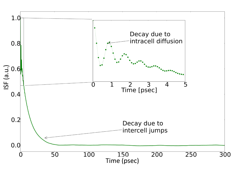
Figure 1: Example of an ISF function. The inset shows the ISF at short times, where a combination of decaying oscillations as well as a decaying exponential can be seen. Their origin is explained in the text.

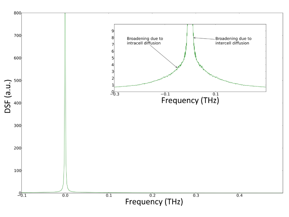
Figure 2: Example of a DSF function calculated from the ISF shown in figure 1, focusing on the two peaks which are located at the origin. The much sharper QEP dominates the DSF, whereas the underlying broad QEB can be seen more clearly in the inset plot.

The slow exponential decay is due to intercell diffusion i.e. transitions between local minimum in a corrugated potential as was discussed in section 2. The quasi-elastic broadening, (or the decay rate of the ISF), $\Gamma$, and its dependence on $\Delta K$ and T can be related to the dynamics either using simple analytical theory (e.g. equation 4) or as will be demonstrated below using more detailed numerical models. In the following section we will use $\Gamma\left(\Delta K,T\right)$ to compare the diffusion process calculated by the two numerical simulations.

The oscillation and decay seen at short time scales, is related to the motion within the adsorption site. The oscillation period reflects the vibrational motion of the adsorbate whereas the fast decay reflects the loss of phase coherency due to the random nature of this motion, a process sometimes referred to as intra-cell diffusion [28, 27]. In the DSF this intra-cell motion appears as three peaks, two inelastic peaks located at the energy gain / loss values which correspond to vibrational frequency and one additional peak centered at $\omega=0$, as shown in figure (2). The width of all three peaks is related to the rapid decay due to the phase loss of the intra-cell motion mentioned above. Since this decay is typically much faster than that due to the inter-cell motion, the widths of all three peaks are substantially larger than that of the QEP (i.e. the quasi-elastic broadening). In this work we will refer to the intra-cell motion contribution centered at $\omega=0$ as the quasi-elastic base (QEB) to differentiate it from the much sharper QEP which is also centered at $\omega=0$. As mentioned above, in many cases the time scale of the intercell diffusion is much slower compared to the intra-cell one, and the differentiation of the different contributions mentioned above is valid. In section 4.1.1 we will make use of this separation scheme in order to extract values for the frictional coupling within the adsorption site.

4 Comparison of MD and Langevin quasi-elastic broadenings

As mentioned above, under many circumstances, including the conditions encountered in this work, inter-cell motion leads to an exponentially decaying ISF equivalent to a Lorentzian QEP in the DSF. Under these conditions, the quasi-elastic broadening $\Gamma$, which can be extracted either from the decay rate of the ISF or from the width of the QEP peak in the DSF, can be used to characterize the inter-cell motion from both experiments and theory [3, 4, 5]. A method which allowed us to reliably extract , $\Gamma$, from the calculated ISF is to delay the fitting procedure to times which are sufficiently long to avoid mixing the contributions of the intra-cell motion mentioned above. .

We start with the case of an adsorbate with a mass of 23 amu, representing the Na/Cu(001) system mentioned earlier. Figure 3 shows a comparison of $\Gamma$ calculated using the two simulation approaches. The left panel shows an example for calculations performed at 160K, the MD results are shown using the black dot symbols, where as Langevin results using different friction values in the range 0.44THz-0.72THz are plotted with coloured symbols according to the legend. One immediate feature which can be seen for both simulations is the oscillatory nature of the width of the QEP as function of the momentum transfer value. This is a characteristic feature of jump diffusion as can be seen from the Chudley Elliot equation (4). A second observation which can be made is that the Langevin simulation can reproduce the MD result quite well if the friction parameter is set to a value of 0.56THz , we will refer to the friction parameter which provides the best fit as the “optimal friction value”, $\eta_{opt}$ . This particular value is consistent with the results obtained in the past when analyzing experimental measurements of Na/Cu(001) with Langevin simulations [18, 17]. For lower friction values we observe a slower jump rate due to weak coupling between the substrate and adsorbate, while for higher friction values the shape of the curve is narrower, indicating the dominance of single jumps (equation (4) reverts to a single oscillating term when only nearest neighbor jumps take place).

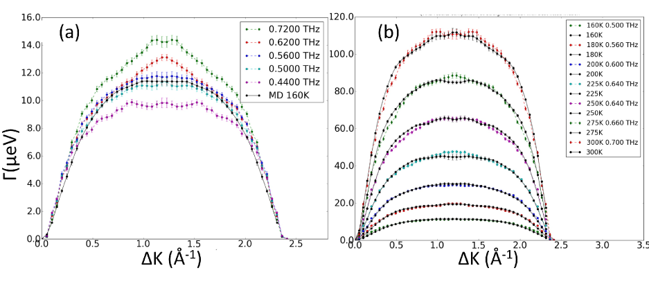
Figure 3: a) Quasi-elastic broadening, $\Gamma\left(\Delta K\right)$, calculated along the (1,1,0) crystal azimuth for a 23 amu adsorbate at 160K. MD results are shown with full black circles alongside with the results of Langevin simulations with different friction parameters as indicated in the legend. b) Comparison between the $\Gamma\left(\Delta K\right)$ calculated by the MD (black circles) and those calculated by the Langevin using the optimal friction values indicated in the legend alongside the relevant surface temperature.

The right panel of figure 3 shows the same comparison in the temperature range 140K-300K. For each temperature we plot the MD calculation together with the Langevin simulation obtained using the optimal friction values, $\eta_{opt}(T)$, i.e. the friction values which gave the minimal standard deviation between the two $\Gamma\left(\Delta K\right)$ curves. Again one can see that the Langevin simulation can reproduce the MD values quite well, however, the optimal friction parameters (indicated in the legend) are not identical for the different temperatures, instead there is a subtle but clear trend where the friction parameter, $\eta_{opt}$, increases with the temperature, i.e. the Langevin simulation we used can not exactly reproduce the MD results if a single temperature independent friction value is used.

4.1 Temperature dependent friction

In the previous section we saw that we can find a good agreement between the quasi-elastic broadenings, $\Gamma\left(\Delta K,T\right)$, calculated by the two numerical models with only one free parameter, $\eta$ - the frictional coupling. However, in order to optimize the fit we had to slightly adjust the friction according to the temperature. During the last two decades various systems have been measured using QHAS, most of which were analyzed using Langevin simulations where a single, temperature independent, friction coefficient was assumed [3, 4, 5]. If the temperature dependence of the friction is significant for some of these systems, the analysis method which was applied in the past to extract an activation energy for these systems, resulted in a small but systematic error which needs to be taken into account. In order to study and understand this apparent temperature dependence we performed further calculations for heavier adsorbates, as this allows us to change the strength of the frictional coupling [29, 30] while leaving the inter-atomic forces unchanged. Figure 4 shows the friction values which give the best quasi-elastic broadening match between the two simulations at different temperatures for 100 amu and 200 amu adsorbates. The resolution of the friction parameter is $5GHz$ and $2GHz$ for the 100 and 200 amu masses respectively.

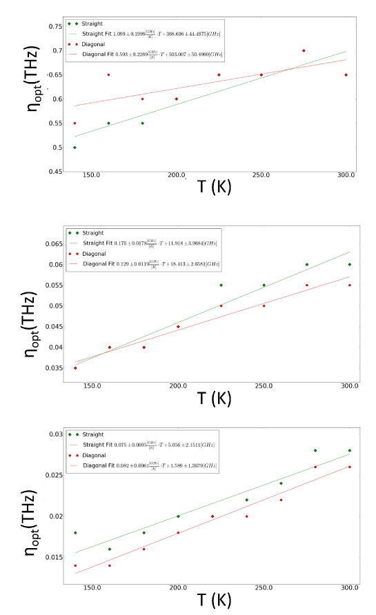
Figure 4: From top to bottom: The optimal friction as a function of temperature for 23, 100 and 200 amu adsorbates respectively. Results for the ”straight” (over the bridge site) crystal azimuth (110) are plotted in green and results for the ”diagonal” (over the top) azimuth (100) in red. A linear form was fitted for both crystal azimuths. Note that the relative change of the optimal friction parameter in the temperature range 150-300K can be as large as 100% for the heavier adsorbates we simulated.

Two Main observations can be made when comparing the results of the different masses: i) The friction values needed to fit the two simulations are significantly reduced for heavier adsorbates. This is the expected trend, since heavier adsorbates have a lower vibration frequency and are expected to have a weaker coupling to the substrate [29, 30]. ii) The need to adjust the friction parameter according to the temperature in order to get an agreement between the two simulations is more pronounced for the heavier adsorbates. Thus, this temperature dependent friction which is rather subtle for the 23 amu adsorbate, and would have a small effect on the interpretation of experimental data , becomes a more significant effect for heavier adsorbates.

4.1.1 Estimating the friction from the MD simulation

We have shown above, that in order to mimic the MD results using a Langevin simulation we need to allow the friction parameter to increase with temperature. One explanation for this is that by changing the friction we simply make use of our only free parameter to compensate for the fact that the Langevin simulation can not exactly mimic the MD results, either due to the fundamental differences between the two, or due to our particular choice for the PES. On the other hand, since the friction is not an explicit parameter in the MD simulation, another possibility is that the friction coupling changes with temperature in the MD simulation and that the comparison with the Langevin simulation is revealing this trend. In order to try and differentiate between these possibilities we have attempted to extract an effective “friction parameter” from the MD simulation and study its temperature dependence.

We achieve this by extracting the width of the quasi-elastic base (QEB), as mentioned in section (2). The width of the QEB is governed by the dephasing rate of the intracell motion, i.e. it is related to the friction coupling within the adsorption site, a relation which has been shown, both analytically and numerically [27, 31]. In fact, if one looks at the lowest order of the analytically derived expression for the DSF, the half width of the QEB (in the angular frequency domain) is simply equal to $\eta$ [31].

While the QEB width will undoubtedly be related to the frictional coupling, the accuracy of the simple relation between the two mentioned above is unknown. In particular, the analytical relation is valid within certain approximations [31]. Furthermore, the friction in the Langevin simulation reflects the average energy exchange rate, both within and outside the adsorption site, whereas the QEB is only related to the intracell motion within the adsorption site, hence the two properties are obviously not identical. In order to validate our approach, we first start by applying this method on the DSF calculated by Langevin. Since Langevin simulations include an explicit friction value, our ability to reproduce this value from the QEB acts as a self consistency check for our method.

In order to assist the fitting procedure and separate any contributions from intercell diffusion, the DSF calculations were performed along the straight azimuth for $\Delta K\approx 2.46\AA$, conditions under which the QEP has a negligible width due to the jump diffusion process (minima values of $\Gamma$ in eq. 4). . The fit for the Langevin data is shown in figure (5). At each temperature, the DSF corresponds to a calculation using the optimal friction value from figure (4). The inset in figure (5) shows the friction values extracted from the QEB width (blue circles) versus the friction parameters used in the simulation (denoted $\eta_{opt})$ . Overall, the two values are very close, with the QEB underestimating the friction parameters by 15%-20%, similar calculation for higher masses (100 amu and 200 amu, data not shown) produce even smaller deviations between the two. Thus, we conclude that the QEB width provides a reasonable way to estimate the friction within the accuracy stated above.

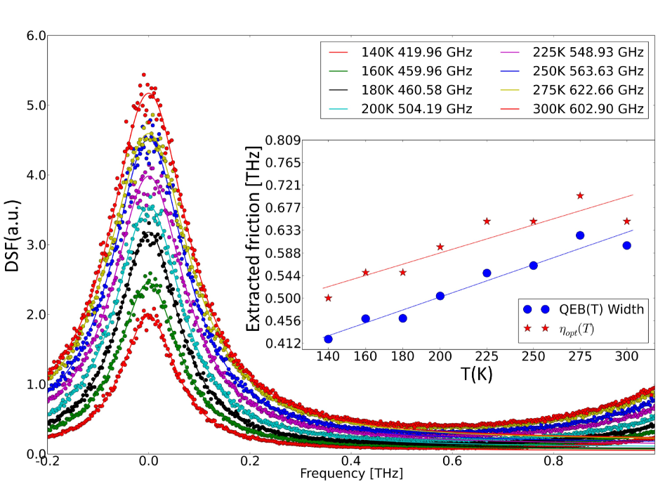
Figure 5: Fitting the QEB peak calculated by the Langevin simulations for the different temperatures. The full symbols are the DSF values calculated by the Langevin simulations, performed using $\eta_{opt}$ friction parameters. The solid lines show the Lorentzian fit described in the text which was used to extract the QEB width. The inset compares $\eta_{opt}$ with the friction values extracted from the width of the Lorentzian peak which best fitted the QEB[31].

Next, we applied the same procedure on the MD data in order to extract effective friction values and check how they change with temperature. Figure 6 shows the QEB peaks calculated for the different temperatures and different adsorbate masses, and a Lorentzian peak fit (full lines) to the QEB. First we note, that the Lorentzian fit to the QEB peak is not quite as good as it was for the spectra calculated by the Langevin simulation, mostly due to low frequency peaks related to the surface vibrations and an incomplete subtraction of the QEP peak (assumed to be a delta function at the diffraction condition). Nevertheless, we see that the values extracted from the Lorentzian width are quite close to the Langevin friction values which were obtained by fitting the $\Gamma\left(\Delta K\right)$ curves ($\eta_{opt}$). The inset depicts the comparison between $\eta_{opt}$ and QEB widths (extracted from the MD simulation) for the different temperatures and adosrbate masses. An obvious feature which can be seen from these graphs is that for all three masses the QEB widths extracted from the MD calculations increase as function of temperature, more or less following the trend of $\eta_{opt}$. Consequently , we conclude that the need to increase $\eta_{opt}$ as function of T when trying to reproduce the MD results with the Langevin simulation, represents a property of the frictional coupling of the MD simulation, which is then revealed in the comparison with the Langevin simulations. In other words, the fact we had to increase $\eta_{opt}$ with temperature in order to mimic the MD results with the Langevin code, does not indicate a discrepancy between the two simulations.

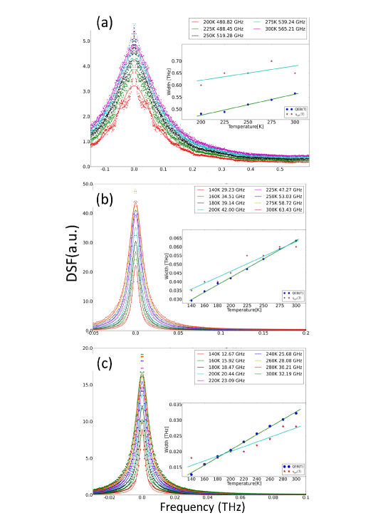
Figure 6: From top to bottom, results of the $QEB_{MD}(T)$ fit to a single Lorentzian for 23, 100 and 200 amu adsorbate. The inset shows the QEB widths extracted from MD data simulations at different temperatures alongside the optimal friction values, $\eta_{opt}$, used by the Langevin simulation to fit the MD $\Gamma\left(\Delta K\right)$ curves .

5 Summary and Conclusions

We have compared two different numerical approaches for interpreting adsorbate diffusion on a solid substrate, namely, MD and Langevin simulations. A major difference between these two approaches is the substitution of the dynamic substrate which is explicitly simulated by the MD code, with a friction damping term and a stochastic force in the Langevin simulation. Since this substitution can not accurately account for correlations between the relative motion of the substrate and adsorbate atoms which takes place in the MD, a certain discrepancy in the simulated dynamics is anticipated. For example, a substrate phonon creates a time dependent distortion of the potential energy surface on which the adsorbate moves, hence one could expect that the rate of single jumps and longer jumps would be affected by the frequency and amplitude of the substrate vibrations. While it is obvious that such correlations will take place to some degree, a quantitative assessment of the discrepancies was missing in the literature, and it was unclear whether they are sufficiently large to affect the interpretation of realistic (noisy) experimental data. The observables we chose to compare are the ISF and DSF correlation functions, focusing on the width of the quasi-elastic peak, $\Gamma$, in particular. The dependence of the quasi-elastic peak width on the momentum transfer and sample temperature provides a sensitive measure of the motion rate and mechanism, and is also accessible to helium scattering experiments[3, 4, 5].

The comparison we performed showed that for the particular systems we simulated, the two simulations can produce very similar observables, using the friction parameter as the only free parameter used to fit the two. Thus, within the conditions we simulated, correlation effects do not seem to lead to any noticeable discrepancies between the two simulations, and the Langevin simulations provides a good approach for simulating the surface dynsmics.

We did notice that the optimal friction values which we obtained from fitting the two simulations increased slightly with temperature, an effect which was more significant for adsorbates with a higher mass. One possible interpretation of this observation is that the need to increase the friction parameter of the Langevin simulation at higher temperatures is an indication of a discrepancy between the two numerical approaches (i.e. we are compensating for fundamental differences between the two simulations by adjusting the fit parameter). Another interpretation is that the frictional coupling rate is increasing with temperature in the MD simulation and that the comparison with the Langevin simulation (which produces an optimal friction parameter) is simply revealing this fact. We used the quasi-elastic base width as a method to estimate the frictional coupling from the dephasing rate of the motion within the adsorption site and extract effective friction values from the MD data. Our results show that the effective friction values extracted using this method, are in close proximity to those used to fit the Langevin simulation. Furthermore, the effective friction values also show an increase with temperature supporting the second interpretation mentioned above, i.e the frictional coupling increases with temperature in the MD simulation and the need to adjust the friction parameter of the Langevin simulation to fit the two simulations does not indicate a discrepancy between the two numerical approaches.

In conclusion, when using the particular interaction models mentioned above, adsorbate masses ranging from 23 to 200 amu, and temperatures within the range of 140K to 300K, we do not observe significant differences between the Langevin and MD simulations. Thus, even if differences exist, they are subtle and should not affect the analysis of experimental data with similar or larger noise levels. An explanation for this lack of discrepancy, might be that the relatively fast time scales which characterize the substrate motion lead to an averaging effect which reduces the importance of explicit correlations and allows us to treat the interaction as a sum of a static interaction (PES) and a stochastic force with a good accuracy. It is also worth noting, that in the past when applying Langevin simulations for data analysis, it was assumed that the friction is independent of surface temperature. While the particular trend we observed in the MD simulation reflects our choice of model for simulating the substrate (harmonic potential) and adsorbate (Morse potential) and is not directly related to other systems and interaction models, it is worth remembering that the friction might change as function of temperature also in other systems. If this temperature dependence is not negligible and is not taken into account, systematic errors might be produced when extracting physical properties from the simulations, in particular the energy barrier for diffusion deduced from Arrhenius graphs. Finally, we assume that there will be other systems and conditions under which correlations will produce noticeable effects, however, these will probably require substantially different time scales (faster adsorbate motion or slower substrate motions) and it should be interesting to study such systems in the future.

6 Acknowledgements

The authors would like to thank Prof. Erio Tossati for valuable scientific discussions. This work was supported by the Israeli Science Foundation (Grant No. 2011185) and the European Research Council under the European Union’s seventh framework program (FP/2007- 2013)/ ERC Grant 307267.

References

- [1] Grazyna Antczak and Gert Ehrlich. Surface Diffusion. Cambridge University Press, 2010.
- [2] T. Ala-Nissila, R. Ferrando, and S. C. Ying. Collective and single particle diffusion on surfaces. Advances in Physics, 51(3):949, 2002.
- [3] G Alexandrowicz and A P Jardine. Helium spin-echo spectroscopy: studying surface dynamics with ultra-high-energy resolution. Journal of Physics: Condensed Matter, 19(30):305001, August 2007.
- [4] A. P. Jardine, G. Alexandrowicz, H. Hedgeland, W. Allison, and J. Ellis. Studying the microscopic nature of diffusion with helium-3 spin-echo. Physical Chemistry Chemical Physics, 11(18):3355, 2009.
- [5] A.P. Jardine, H. Hedgeland, G. Alexandrowicz, W. Allison, and J. Ellis. Helium-3 spin-echo: Principles and application to dynamics at surfaces. Progress in Surface Science, 84(11-12):323–379, November 2009.
- [6] J. Ellis and J.P. Toennies. A molecular dynamics simulation of the diffusion of sodium on a cu(001) surface. Surface Science, 317(1-2):99–108, September 1994.
- [7] Peter Fouquet, Mark R. Johnson, Holly Hedgeland, Andrew P. Jardine, John Ellis, and William Allison. Molecular dynamics simulations of the diffusion of benzene sub-monolayer films on graphite basal plane surfaces. Carbon, 47(11):2627–2639, 2009.
- [8] A. P. Jardine, E. Y. M. Lee, D. J. Ward, G. Alexandrowicz, H. Hedgeland, W. Allison, J. Ellis, and E. Pollak. Determination of the quantum contribution to the activated motion of hydrogen on a metal surface: H/Pt(111). Physical Review Letters, 105(13):136101, 2010.
- [9] Ellen H. G. Backus, Andreas Eichler, Aart W. Kleyn, and Mischa Bonn. Real-time observation of molecular motion on a surface. Science, 310(5755):1790 –1793, December 2005.
- [10] Leon Van Hove. Correlations in space and time and born approximation scattering in systems of interacting particles. Physical Review, 95(1):249, July 1954.
- [11] E. Hulpke and G. Benedek. Helium atom scattering from surfaces. Springer series in surface sciences. Springer-Verlag, 1992.
- [12] Andrew P Graham. The low energy dynamics of adsorbates on metal surfaces investigated with helium atom scattering. Surface Science Reports, 49(4–5):115 – 168, 2003.
- [13] C T Chudley and R J Elliott. Neutron scattering from a liquid on a jump diffusion model. Proceedings of the Physical Society, 77(2):353–361, February 1961.
- [14] G. Alexandrowicz, A. P. Jardine, P. Fouquet, S. Dworski, W. Allison, and J. Ellis. Observation of microscopic CO dynamics on cu(001) Using^3He spin-echo spectroscopy. Physical Review Letters, 93(15):156103, October 2004.
- [15] V. Rosato, M. Guillope, and B. Legrand. Thermodynamical and structural properties of f.c.c. transition metals using a simple tight-binding model. Philosophical Magazine A, 59(2):321–336, 1989.
- [16] J. Ellis and J.P. Toennies. Observation of jump diffusion of isolated sodium atoms on a cu(001) surface by helium atom scattering. Physical Review Letters, 70(14):2118–2121, 1993.
- [17] A. P. Graham, F. Hofmann, J. P. Toennies, L. Y. Chen, and S. C. Ying. Experimental and theoretical investigation of the microscopic vibrational and diffusional dynamics of sodium atoms on a cu(001) surface. Physical Review B, 56(16):10567, October 1997.
- [18] G. Alexandrowicz, A. P. Jardine, H. Hedgeland, W. Allison, and J. Ellis. Onset of 3D collective surface diffusion in the presence of lateral interactions: Na/Cu(001). Physical Review Letters, 97(15):156103, October 2006.
- [19] Harrison C. White. Atomic force constants of copper from feynman’s theorem. Physical Review, 112(4):1092, November 1958.
- [20] E. C. Svensson, B. N. Brockhouse, and J. M. Rowe. Crystal dynamics of copper. Physical Review, 155(3):619, March 1967.
- [21] D. Frenkel and B. Smit. Understanding Molecular Simulation: From Algorithms to Applications. Computational science series. Elsevier Science, 2001.
- [22] R Kubo. The fluctuation-dissipation theorem. Reports on Progress in Physics, 29(1):255, 1966.
- [23] Gil Alexandrowicz, Pepijn R. Kole, Everett Y. M. Lee, Holly Hedgeland, Riccardo Ferrando, Andrew P. Jardine, William Allison, and John Ellis. Observation of uncorrelated microscopic motion in a strongly interacting adsorbate system. Journal of the American Chemical Society, 130(21):6789–6794, May 2008.
- [24] Guido Fratesi. Potential energy surface of alkali atoms adsorbed on cu(001). Phys. Rev. B, 80:045422, Jul 2009.
- [25] Jacqueline Krim. Friction and energy dissipation mechanisms in adsorbed molecules and molecularly thin films. ADVANCES IN PHYSICS, 61(3):155–323, 2012.
- [26] H. Hedgeland, P. Fouquet, A. P. Jardine, G. Alexandrowicz, W. Allison, and J. Ellis. Measurement of single-molecule frictional dissipation in a prototypical nanoscale system. Nat Phys, 5(8):561–564, 2009.
- [27] A P Jardine, H Hedgeland, D Ward, Y Xiaoqing, W Allison, J Ellis, and G Alexandrowicz. Probing molecule surface interactions through ultra-fast adsorbate dynamics: propane/pt(111). New Journal of Physics, 10(12):125026, 2008.
- [28] A. P. Jardine, J. Ellis, and W. Allison. Effects of resolution and friction in the interpretation of qhas measurements. The Journal of Chemical Physics, 120(18):8724–8733, 2004.
- [29] B. N. J. Persson and R. Ryberg. Brownian motion and vibrational phase relaxation at surfaces: Co on ni(111). Phys. Rev. B, 32:3586–3596, Sep 1985.
- [30] O. M. Braun and R. Ferrando. Role of long jumps in surface diffusion. Phys. Rev. E, 65:061107, Jun 2002.
- [31] J. L. Vega, R. Guantes, S. Miret-Artés, and D. A. Micha. Collisional line shapes for low frequency vibrations of adsorbates on a metal surface. The Journal of Chemical Physics, 121(17):8580–8588, 2004.