Modelling aggregation on the large scale and regularity on the small scale in spatial point pattern datasets

Abstract

We consider a dependent thinning of a regular point process with the aim of obtaining aggregation on the large scale and regularity on the small scale in the resulting target point process of retained points. Various parametric models for the underlying processes are suggested and the properties of the target point process are studied. Simulation and inference procedures are discussed when a realization of the target point process is observed, depending on whether the thinned points are observed or not. The paper extends previous work by Dietrich Stoyan on interrupted point processes.

Boolean model, chi-square process, dependent thinning, determinantal point process, interrupted point process, pair correlation function.

1 Introduction

In the spatial point process literature, analysis of spatial point pattern datasets are often classified into three main cases (see e.g. Cressie (1993), Diggle (2003), and Møller and Waagepetersen (2004)):

1. Regularity (or inhibition or repulsiveness)—modelled by Gibbs point processes (Ruelle, 1969; Lieshout, 2000; Chiu et al., 2013), Matérn hard core models of types I-III (Matérn, 1986; Møller et al., 2010), other types of hard core processes (Illian et al., 2008), and determinantal point processes (Macchi, 1975; Lavancier et al., 2015).

2. Complete spatial randomness—modelled by Poisson point processes (Kingman, 1993).

3. Aggregation (or clustering)—modelled by Poisson cluster processes (Daley and Vere-Jones, 2003), Cox processes (Cox, 1972), and permanental point processes (Macchi, 1975; McCullagh and Møller, 2006).

A popular and simplistic way to determine (i)-(iii) is in terms of the so-called pair correlation function (Illian et al., 2008): Denote $\rho$ and $g$ the intensity and pair correlation functions for a spatial point process defined on the $d$-dimensional Euclidean space $\mathbb{R}^{d}$ (with $d=2$ or $d=3$ in most applications; formal definitions of $\rho$ and $g$ are given in Section 2.1). For ease of presentation, we assume second order stationarity and isotropy, i.e. $\rho$ is constant and for any locations $x_{1},x_{2}\in\mathbb{R}^{d}$, $g(x_{1},x_{2})=g_{0}(r)$ depends only on the distance $r=\|x_{1}-x_{2}\|$. Intuitively, $\rho\,\mathrm{d}x$ is the probability that the process has a point in an infinitesimally small region of volume (Lebesgue measure) $\mathrm{d}x$, and for $r=\|x_{1}-x_{2}\|>0$, $g_{0}(r)\rho^{2}\,\mathrm{d}x_{1}\,\mathrm{d}x_{2}$ is the probability that the process has a point in each of an infinitesimally small region around $x_{1},x_{2}$ of volumes $\mathrm{d}x_{1},\,\mathrm{d}x_{2}$. Typically, $g_{0}(r)$ tends to 1 as $r\rightarrow\infty$, and we are usually interested in the behaviour of $g_{0}(r)$ for small and modest values of $r$. We expect in case of (i), $g_{0}(r)<1$ when $r$ is small, and $g_{0}(r)$ is less than or fluctuating around 1 otherwise; in case of (ii), $g_{0}=1$; and typically, in case of (iii), $g_{0}>1$.

For applications the classification (i)-(iii) can be too simplistic, and there is a lack of useful spatial point process models with, loosely speaking, aggregation on the large scale and regularity on the small scale. One suggestion of such a model is a dependent thinning of e.g. a Poisson cluster point process where the thinning is similar to that in a Matérn hard core process (see Andersen and Hahn (2015)) or to that in spatial birth-death constructions for Gibbs point processes (see Kendall and Møller (2000) and Møller and Waagepetersen (2004)). Theoretical expressions for intensity and pair correlation of such Matérn thinned point processes have been derived by Palm theory, and their numerical evaluation can be obtained by approximations, cf. Andersen and Hahn (2015), while the spatial birth-death constructions are mathematical intractable. Another possibility is to consider a Gibbs point process with a well-chosen potential that incorporates inhibition at small scales and attraction at large scales. A famous example is the Lennard-Jones pair-potential (Ruelle, 1969), and other specific potentials of this type can be found in Goldstein et al. (2015). Unfortunately, in general for Gibbs point processes the intensity and the pair correlation function are unknown and simulation requires elaborate MCMC methods (Møller and Waagepetersen, 2004).

This paper discusses instead a model for a spatial point process $X$ obtained by an independent thinning of a spatial point process $Y$ where the selection probabilities are given by a random process $\Pi=\{\Pi(x):x\in\mathbb{R}^{d}\}\subseteq[0,1]$: We view $X$ and $Y$ as random locally finite subsets of $\mathbb{R}^{d}$, and let

$$X=\{x\in Y:\Pi(x)\geq U(x)\}$$ (1)

where $U=\{U(x):x\in\mathbb{R}^{d}\}$ consists of independent uniformly distributed random variables between 0 and 1, and where $Y,\Pi,U$ are mutually independent. Dietrich Stoyan (Stoyan, 1979; Chiu et al., 2013) called $X$ an interrupted point process, which we agree is a good terminology when each $\Pi(x)$ is either 0 or 1; indeed, in all Stoyan’s examples of applications, this is the case, though the general theory presented is not making this restriction. Clearly, $\Pi$ should not be deterministic, because then the pair correlation functions for $X$ and $Y$ would be identical ($g_{X}=g_{Y}$). We have in mind that a realization of $X$ is observed within a bounded window $W$, while we treat $(\Pi,U)$ as being unobserved, and $Y$ as being or not being observed within $W$. For instance, we can think of $Y$ as describing an inhibitive behaviour of some plant locations under optimal conditions, and $X$ as the actual plant locations due to unobserved covariates (e.g. light conditions, level of water underground, and quality of soil).

Our idea is that it is possible to choose models for $Y$ from the class (i) above together with models for $\Pi$ such that $X$ exhibits small scale regularity and large scale aggregation. Some examples of simulated realizations of this kind of models are shown in Figure 1. Our idea is demonstrated in Sections 3-5 and it can be briefly understood as follows. Section 2.1 establishes a simple relationship between the pair correlation functions for $X$ and $Y$: For simplicity, assume second order stationarity and isotropy of both $Y$ and $\Pi$, whereby our target point process $X$ becomes second order stationary and isotropic. The (isotropic) pair correlation function of $X$ is given by

$$g_{X,0}(r)=M_{0}(r)g_{Y,0}(r)$$ (2)

where, setting $0/0=0$,

$$M_{0}(r)=M(x_{1},x_{2})=\frac{\mathrm{E}[\Pi(x_{1})\Pi(x_{2})]}{\mathrm{E}[\Pi(x_{1})]\mathrm{E}[\Pi(x_{2})]},\quad x_{1},x_{2}\in\mathbb{R}^{d},$$ (3)

depends only on $r=\|x_{1}-x_{2}\|$. For example, if $\Pi$ is positively correlated (i.e. $M_{0}>1$) and $Y$ is a determinantal point process (this process is described in Section 2.2), then $g_{Y,0}\leq 1$ and in accordance with (2) we may obtain a behaviour of $g_{X,0}$ as we wish, namely that $g_{X,0}$ is smaller respective larger than 1 on the small respective large scale. Examples appear later in Figure 2.

Figure 1: Examples of realizations within a unit square of $X$ given by the models 1.-4. in Section 4.3: In the first row $Y$ is a determinantal point process, in the second row $Y$ is a Matérn hard core process of type II, in the first column $-\log\Pi$ is a $\chi^{2}$-process, and in the second column $\Pi$ is the characteristic function for a Boolean disc model.

We thank Ute Hahn for reminding us about Stoyan’s interrupted point process in Stoyan (1979), Chiu et al. (2013), and Kautz et al. (2011). In Stoyan (1979) and Chiu et al. (2013) he considered mainly the planar case where $Y$ is a Matérn hard core process of type II and where $\Pi$ is the characteristic function of a motion invariant random closed set whose distribution apart from $\mathrm{E}[\Pi(o)]$ and $M_{0}(r)$ is unspecified ($o$ denotes the origin in $\mathbb{R}^{d}$). In contrast we consider various models for both $Y$ and $\Pi$, where e.g. our $\chi^{2}$-process model for $-\log\Pi$ seems more realistic for applications like the example studied in Section 5.1. Moreover, we discuss simulation and parametric inference procedures depending on whether $Y$ is observed or is a latent process. Finally, we notice that the paper Kautz et al. (2011) is in another direction than ours, since they consider $Y$ to be a Matérn cluster process (which is of class (iii) above) and $\Pi$ to be the characteristic function for a motion invariant random closed set, i.e. $X$ becomes of class (iii).

Our paper is organized as follows. Section 2 recalls some background material and deals with some inhibitive point process models for $Y$ where $\rho_{Y}$ and $g_{Y,0}$ are known, namely determinantal point processes and Matérn hard core models of type I or II. Section 3 introduces models for $\Pi$, based on transformed Gaussian processes and Boolean models, which combined with the models for $Y$ allow us to further study the behaviour of $g_{X,0}$. Section 4 discusses first simulation of $(Y,\Pi,X)$, and second inference for parametric models for $Y$ and $\Pi$, depending on whether $Y$ is observed or not. Finally, Section 5 fits parametric models to examples of spatial point pattern datasets using the methodology from Section 4.

2 Preliminaries

Let the situation be as in Section 1. This section recalls the definitions and some properties of product densities for a spatial point process in general and for determinantal point processes and Matérn hard core models of types I-II in particular.

2.1 Product densities and assumptions

For $n=1,2,\ldots$, suppose that $\rho^{(n)}_{Y}:\mathbb{R}^{dn}\mapsto[0,\infty)$ is a Borel function satisfying the so-called Campbell formula

$$\mathrm{E}\sum_{x_{1},\ldots,x_{n}\in Y}^{\not=}f(x_{1},\ldots,x_{n})=\int\cdots\int f(x_{1},\ldots,x_{n})\rho_{Y}^{(n)}(x_{1},\ldots,x_{n})\,\mathrm{d}x_{1}\cdots\,\mathrm{d}x_{n}$$ (4)

for any non-negative Borel function $f$, where $\sum^{\not=}$ means that $x_{1},\ldots,x_{n}$ are pairwise distinct. Then $\rho^{(n)}_{Y}$ is called an $n$th order product density of $Y$. Such a function is apart from a Lebesgue nullset uniquely determined by the Campbell formula. Henceforth, for ease of presentation, we ignore nullsets. In particular, $\rho_{Y}=\rho_{Y}^{(1)}$ is the intensity function. Furthermore, setting $0/0=0$, the pair correlation function is defined by $g_{Y}(x_{1},x_{2})={\rho_{Y}^{(2)}(x_{1},x_{2})}/[{\rho_{Y}(x_{1})\rho_{Y}(x_{2})}]$. The usual practice is to set $\rho^{(n)}_{Y}(x_{1},\ldots,x_{n})=0$ if $x_{i}=x_{j}$ for some $i\not=j$. An exception is the case of a Poisson process $Y$ where often one takes $\rho_{Y}^{(2)}(x_{1},x_{2})=\rho_{Y}(x_{1})\rho_{Y}(x_{2})$ so that $g_{Y}(x_{1},x_{2})=1$ if $\rho_{Y}(x_{1})\rho_{Y}(x_{2})>0$.

Recall that we assume for simplicity that $Y$ is second order stationary and isotropic. We also assume that the first and second order intensity functions exist. Thus we can consider the versions where $\rho_{Y}$ is constant and where $g_{Y}(x_{1},x_{2})=g_{Y,0}(r)$ depends only on the distance $r=\|x_{1}-x_{2}\|$. We call $g_{0}$ the isotropic pair correlation function. We furthermore assume $\rho_{Y}>0$ (otherwise $Y$ is empty, which is not a case of interest).

Similarly, $\rho^{(n)}_{X}$ and $g_{X,0}$ denote the $n$th order product density and the isotropic pair correlation function of $X$. By conditioning on $Y$ and using (1) and (4) it is straightforwardly verified that $\rho^{(n)}_{X}$ exists whenever $\rho^{(n)}_{Y}$ exists, in which case

$$\rho^{(n)}_{X}(x_{1},\ldots,x_{n})=\mathrm{E}[\Pi(x_{1})\cdots\Pi(x_{n})]\rho^{(n)}_{Y}(x_{1},\ldots,x_{n}).$$

Consequently, for any $r\geq 0$,

$$\rho_{X}=q\rho_{Y},\quad g_{X,0}(r)=M_{0}(r)g_{Y,0}(r),$$ (5)

where $q=\mathrm{E}[\Pi(o)]$ denotes the mean selection probability. Equation (5) is similar to results given in Stoyan (1979).

For later purposes, denote $\bar{X}=Y\setminus X$ the complementary set of $X$ in $Y$. Then, using an obvious notation,

$$\rho^{(n)}_{\bar{X}}(x_{1},\ldots,x_{n})=\mathrm{E}[(1-\Pi(x_{1}))\cdots(1-\Pi(x_{n}))]\rho^{(n)}_{Y}(x_{1},\ldots,x_{n})$$

and hence by (3) and (5),

$$\rho_{\bar{X}}=(1-q)\rho_{Y},\quad g_{\bar{X},0}(r)=\frac{1-2q+q^{2}M_{0}(r)}{(1-q)^{2}}\,g_{Y,0}(r).$$ (6)

Finally, the cross pair correlation between $X$ and $\bar{X}$ (see e.g. Møller and Waagepetersen (2004) for a definition) is given by

$$g_{X\bar{X},0}(r)=\frac{q-q^{2}M_{0}(r)}{q(1-q)}\,g_{Y,0}(r).$$ (7)

2.2 Determinantal point processes

Let $C$ be a complex function defined on $\mathbb{R}^{d}\times\mathbb{R}^{d}$ and $Y$ be a determinantal point process (DPP) with kernel $C$. By definition this means that for any $n=1,2,\ldots$ and any $x_{1},\ldots,x_{n}\in\mathbb{R}^{d}$, $\rho^{(n)}_{Y}(x_{1},\ldots,x_{n})$ exists and is equal to the determinant of the $n\times n$ matrix with $(i,j)$th entry $C(x_{i},x_{j})$. For background material on DPPs, including conditions for their existence, see Lavancier et al. (2015) and the references therein.

For simplicity and specificity, we assume that $C$ is a stationary and isotropic covariance function, i.e. $C(x,y)=C_{0}(\|x-y\|)$ is real and non-negative definite. Clearly, $Y$ is then a stationary and isotropic DPP, and we write $Y\sim{\mathrm{DPP}}(C_{0})$. We also assume that $C_{0}(\|x\|)$ is continuous and square integrable, i.e. $\int_{0}^{\infty}r^{d-1}|C_{0}(r)|^{2}\,\mathrm{d}r<\infty$. By Theorem 2.3 and Proposition 3.1 in Lavancier et al. (2015), the existence of ${\mathrm{DPP}}(C_{0})$ is then equivalent to that $\varphi_{0}\leq 1$, where

$$\varphi_{0}(r)=\left\{\begin{array}[]{ll}2\int_{0}^{\infty}C_{0}(s)\cos(2\pi rs)\,\mathrm{d}s&\mbox{if $d=1$}\\ \frac{2\pi}{r^{d/2-1}}\int_{0}^{\infty}C_{0}(s)J_{d/2-1}(2\pi rs)s^{d/2}\,\mathrm{d}s&\mbox{if $d=2,3,\ldots$}\end{array}\right.$$

is the spectral density associated to $C_{0}$ and $J_{d/2-1}$ is the Bessel function of order $d/2-1$.

Observe that

$$\rho_{Y}=C_{0}(0)$$ (8)

which is assumed to be strictly positive, and

$$g_{Y,0}(r)=1-{C_{0}(r)^{2}}/{\rho_{Y}^{2}}$$ (9)

is 1 minus the squared correlation function. This implies that $g_{Y}\leq 1$ which is one among many other properties confirming that a DPP is inhibitive, cf. Lavancier et al. (2015) and Biscio and Lavancier (2015).

2.3 Matérn hard core models of types I-II

Following Matérn (1986) we define hard core point processes as follows. Let $\Phi$ be a stationary Poisson process on $\mathbb{R}^{d}$ with intensity $\rho_{\Phi}>0$, $D>0$ a hard core parameter, and $V=\{V(x):x\in\mathbb{R}^{d}\}$ a random process of independent uniformly distributed random variables between 0 and 1, where $\Phi$ and $V$ are independent. Denote $\omega_{d}=\pi^{d/2}/\Gamma(1+d/2)$ the volume of the $d$-dimensional unit ball, and $k_{d}(r,D)$ the volume of the intersection of two $d$-dimensional balls of radii $D$ and distance $r$ between their centres. The Matérn hard core model of type I, denoted $Y_{I}$, is given by the points in $\Phi$ which are not $D$-close to some other point in $\Phi$, i.e.

$$Y_{I}=\{x\in\Phi:\|x-y\|>D\mbox{ whenever $y\in\Phi\setminus\{x\}$}\}.$$

For the Matérn hard core model of type II, denoted $Y_{II}$, we interpret $V(x)$ as the birth time of $x$ and let $Y_{II}$ consist of the points $x\in\Phi$ such that no other $D$-close point in $\Phi$ is older than $x$, i.e.

$$Y_{II}=\{x\in\Phi:\|x-y\|>D\mbox{ whenever $y\in\Phi$ and $V(x)>V(y)$}\}.$$

These hard core point processes are stationary and isotropic with intensities

$$\rho_{Y_{I}}=\rho_{\Phi}\exp\left(-\rho_{\Phi}\omega_{d}D^{d}\right),\quad\rho_{Y_{II}}=\frac{1-\exp\left(-\rho_{\Phi}\omega_{d}D^{d}\right)}{\omega_{d}D^{d}},$$ (10)

and pair correlation functions

$$g_{Y_{I},0}(r)=1(r>D)\exp(\rho_{\Phi}k_{d}(r,D))$$ (11)

and

$$g_{Y_{II},0}(r)= 1[r>D]\frac{2\omega_{d}D^{d}}{\left(\omega_{d}D^{d}-k_{d}(r,D)\right)\left(1-\exp\left(-\rho_{\Phi}\omega_{d}D^{d}\right)\right)}$$

$$\left[1-\frac{1-\exp\left(-\rho_{\Phi}\left(2\omega_{d}D^{d}-k_{d}(r,D)\right)\right)}{\left(2\omega_{d}D^{d}-k_{d}(r,D)\right)\left(1-\exp\left(-\rho_{\Phi}\omega_{d}D^{d}\right)\right)}\omega_{d}D^{d}\right]$$ (12)

where $1(\cdot)$ is the indicator function. Note that $Y_{I}\subseteq Y_{II}$ and $\rho_{Y_{I}}<\rho_{Y_{II}}$. The pair correlation functions in (11)-(12) are continuous except at $r=D$, 0 when $r\leq D$, strictly decreasing for $r\in]D,2D[$, and 1 when $r\geq 2D$. Finally, note that $k_{d}(r,D)=0$ if $r\geq 2D$, and

$$k_{d}(r,D)=\left\{\begin{array}[]{lll}2D-r&\mbox{if $d=1$}\\ 2D^{2}\arccos\left(\frac{r}{2D}\right)-\frac{r}{2}\sqrt{4D^{2}-r^{2}}&\mbox{if $d=2$}\\ \frac{4\pi}{3}D^{3}\left(1-\frac{3r}{4D}+\frac{r^{3}}{16D^{3}}\right)&\mbox{if $d=3$}\end{array}\right.$$ (13)

if $r\leq 2D$.

3 Specific models for the selection probabilities

Section 3.1 discusses the implications of (5) in general, while Sections 3.2-3.3 consider two classes of models for $\Pi$ where explicit expressions for our main characteristics ($q,\rho_{X},M_{0},g_{X,0}$) are available.

3.1 General results and conditions

In the remainder of this paper, to exclude non-interesting cases, we focus on the following situation. We always assume that $\Pi(o)$ has a positive variance or equivalently that $M_{0}(0)>1$, since we do not want $\Pi$ to be deterministic. In addition, we always assume that $\rho_{X}>0$ (or equivalently $\rho_{Y}>0$ and $q>0$), because otherwise $X$ would be almost surely empty. Since it is typically the case that an isotropic pair correlation function tends to 1 as the distance tends to infinity, we want $M_{0}(r)$ to tend to 1 as $r\to\infty$, cf. (5). Therefore we are not so interested in the case where $\Pi(x)$ does not depend on the location $x$, since then $M_{0}$ is a constant $\geq 1$ and $\Pi$ is deterministic if $M_{0}=1$.

We have $g_{X,0}=g_{Y,0}$ if and only if $\Pi$ is uncorrelated, cf. (3) and (5). If $\Pi$ is non-negatively correlated, i.e.  $M_{0}\geq 1$, then $g_{X,0}\geq g_{Y,0}$, so $g_{Y,0}$ cannot cross 1 before $g_{X,0}$ crosses 1. If $\Pi$ is positively correlated, i.e. $M_{0}>1$, then $g_{X,0}>g_{Y,0}$. If $\Pi$ can be negatively correlated, a rather peculiar behaviour of $g_{X,0}$ may happen and we shall exclude this case in our specific models.

By Cauchy-Schwartz inequality and since $\Pi^{2}\leq\Pi$, we have for $r=\|x_{1}-x_{2}\|\geq 0$,

$$M_{0}(r)=\frac{\mathrm{E}\left[\Pi(x_{1})\Pi(x_{2})\right]}{q^{2}}\leq\frac{\sqrt{\mathrm{E}\left[\Pi(x_{1})^{2}\right]}\sqrt{\mathrm{E}\left[\Pi(x_{s})^{2}\right]}}{q^{2}}\leq\frac{\sqrt{\mathrm{E}\left[\Pi(x_{1})\right]}\sqrt{\mathrm{E}\left[\Pi(x_{s})\right]}}{q^{2}}=\frac{1}{q}.$$

Combining this with (5), we obtain an upper bound: $g_{X,0}\leq g_{Y,0}/q$.

Define $\tau_{Y}=\sup\{\tau\geq 0:g_{Y,0}(r)=0\mbox{ whenever }r\leq\tau\}$. When $\tau_{Y}>0$ we say that $Y$ is a hard-core process with hard-core parameter $\tau_{Y}$. Assume that $M_{0}(r)>0$ for all $r\geq 0$; this is satisfied for all the models of $\Pi$ specified later in this paper. Then $\tau_{X}=\tau_{Y}$, cf. (5). Hence $X$ is a hard-core process if and only if $Y$ is a hard-core process.

At the small scale, i.e. when $r\leq\tau$ where $\tau>0$ is a sufficiently small constant, we have the following.

1. Assume $M_{0}$ is continuous. Since $M_{0}(0)>1$, we can assume that $M_{0}(r)>1$ for $r\leq\tau$. Hence, by (5), for $r\leq\tau$, either $g_{X,0}(r)>g_{Y,0}(r)$ or $g_{X,0}(r)=g_{Y,0}(r)=0$.

2. Assume both $M_{0}$ and $g_{Y,0}$ are continuous. Then $g_{X,0}$ is continuous, and so we can assume that $g_{Y,0}\leq g_{X,0}(r)<1$ for $r\leq\tau$. Consequently, at distance $r\leq\tau$, the inhibitive behaviour of $Y$ (quantified in terms of its pair correlation function) is preserved in $X$ but it cannot be stronger.

In brief we will be interested in models where $\Pi$ is positively and not too weakly correlated at the small scale.

At the large scale, basically the properties of $g_{X}$ depends on $q$ and the range of correlation of $\Pi$. If $q$ is large, then since $g_{X,0}\leq g_{Y,0}/q$ we may have $g_{X}\leq 1$, meaning that no clustering is created by the thinning process; an obvious example is when $g_{Y,0}\leq 1$, as e.g. in a DPP. If $q$ is sufficiently small, then $\sup_{r}g_{X}(r)>1$ occurs in our examples of models, and we expect this to be the situation in many other cases. However, it is not true that there always exists $q$ such that $\sup_{r}g_{X}(r)>1$. An obvious counterexample is when $\Pi$ is uncorrelated; other counterexamples may be constructed when the variance $\sigma^{2}$, say, of $\Pi$ is such that $\sigma^{2}/q^{2}\to 0$ as $q\to 0$. On the other hand, assume $q$ is fixed and $\Pi$ is non-negatively correlated, then it is always possible to get $\sup_{r}g_{X}(r)>1$ by increasing the range of correlation of $\Pi$, i.e. making $M_{0}(r)>1$ for $r$ sufficiently large. This is exemplified in Sections 3.2-3.3.

3.2 Transformed Gaussian processes

This section assumes $-\log\Pi$ is the $\chi^{2}$-process given by

$$\Pi(x)=\exp\left(-\frac{1}{2}\sum_{i=1}^{k}Z_{i}(x)^{2}\right),\quad x\in\mathbb{R}^{d},$$ (14)

where $Z_{i}=\{Z_{i}(x):x\in\mathbb{R}^{d}\}$, $i=1,\ldots,k$, are i.i.d. zero-mean real Gaussian processes with covariance function $K:\mathbb{R}^{d}\times\mathbb{R}^{d}\mapsto\mathbb{R}$.

A straightforward calculation yields $\mathrm{E}[\Pi(x)]=1/(1+K(x,x))^{k/2}$ and

$$M(x_{1},x_{2})=\left[\frac{(1+K(x_{1},x_{1}))(1+K(x_{2},x_{2}))}{(1+K(x_{1},x_{1}))(1+K(x_{2},x_{2}))-|K(x_{1},x_{2})|^{2}}\right]^{k/2}.$$

Hence, for $K(x_{1},x_{1})K(x_{2},x_{2})>0$ and defining $R(x_{1},x_{2})=K(x_{1},x_{2})/\sqrt{K(x_{1},x_{1})K(x_{2},x_{2})}$,

$$M(x_{1},x_{2})=\left[1-\frac{R(x_{1},x_{2})^{2}}{(1+1/K(x_{1},x_{1}))(1+1/K(x_{2},x_{2}))}\right]^{-k/2}$$

is an increasing function of $|R(x_{1},x_{2})|,K(x_{1},x_{1}),K(x_{2},x_{2})$, respectively.

In the sequel we assume stationarity and isotropy of $K(x_{1},x_{2})=K_{0}(\|x_{1}-x_{2}\|)$, whereby $\Pi$ is stationary and isotropic. Defining $\kappa=K_{0}(o)$ and $R_{0}=K_{0}/\kappa$, we notice as the variance $\kappa$ increases from zero to infinity that

$$q=1/(1+\kappa)^{k/2}$$ (15)

decreases from 1 to 0, while for fixed $r$,

$$M_{0}(r)=\left[1-\frac{R_{0}(r)^{2}}{(1+1/\kappa)^{2}}\right]^{-k/2}=\left[1-(1-q^{2/k})^{2}R_{0}(r)^{2}\right]^{-k/2}$$ (16)

increases from 1 to $[1-R_{0}(r)^{2}]^{-k/2}$. Thus there is a trade-off between how large $q=\rho_{X}/\rho_{Y}$ and $M_{0}(r)=g_{X,0}(r)/g_{Y,0}(r)$ can be.

We have that $M_{0}(r)\geq 1$ is a decreasing function of $k$ and $M_{0}(r)\to 1$ as $k\to\infty$, showing that taking a large value of $k$ is not appropriate if we want $X$ to exhibit a clustering behaviour at the large scale. Further, assume that the correlation function $R_{0}$ depends on a scale parameter $s>0$, i.e. for all $r\geq 0$, $R_{0}(r)=R_{0}(r,s)=\tilde{R}_{0}(r/s)$ where $\tilde{R}_{0}(r)=R_{0}(r,1)$. This is so for most parametric models of covariance functions used in spatial statistics. Then, for any given $q\in(0,1)$ and $k\geq 1$, we have $M_{0}(r)\to[1-(1-q^{2/k})^{2}]^{-k/2}>1$ as $s\to\infty$ provided $\tilde{R}_{0}$ is continuous at the origin. This combined with (5) proves that $X$ will necessarily exhibit some clustering behaviour at the large scale when $s$ is sufficiently large.

The effect of the parameters is illustrated in Figure 2 which shows the pair correlation of $X$ when $d=2$ and $Y$ is either a DPP or a type II Matérn hard core process. Specifically, the first row of Figure 2 corresponds to the case where $Y$ is a DPP with a Gaussian kernel $C_{0}(r)=\rho_{Y}\exp(-(r/0.015)^{2})$ and $\rho_{Y}=1000$, while in the second row $Y$ is a type II Matérn hard core process with $D=0.015$ and $\rho_{\Phi}=1736$ whereby $\rho_{Y}=1000$. The selection probabilities are given by (14) where $K_{0}$ is a Gaussian covariance function with scale parameter $s$. A joint realization of the restrictions of $Y$, $\Pi$, and $X$ to a unit square is shown on the left hand side of Figure 3.

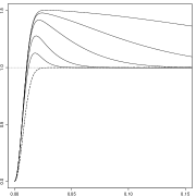
Figure 2: Pair correlation functions of $Y$ (dashed line) and $X$ (solid lines) when $Y$ is a DPP with a Gaussian kernel (first row) or a Matérn hard core process of type II (second row) and $-\log\Pi$ is the $\chi^{2}$-process given by (14) when $K_{0}$ is a Gaussian covariance function with scale parameter $s$. First column: $k=1$, $s=0.05$, and from top to bottom $q=0.4,0.5,0.6,0.7,0.8$; second column: $q=0.5$, $s=0.05$, and from top to bottom $k=1,2,3,5,10$; third column: $q=0.5$, $k=1$, and from top to bottom $s=0.5,0.2,0.1,0.05,0.03$.

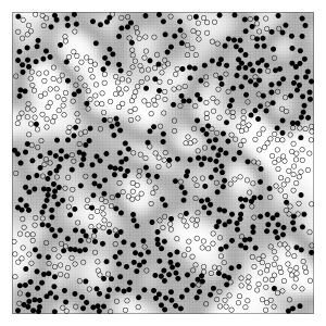
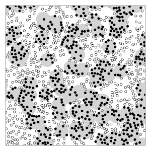
Figure 3: Realization of $Y$ (union of all points) and $X$ (black points) within a unit square when $Y$ is a Matérn hard core process of type II with $\rho_{Y}=1000$ and $D=0.015$. Left: Corresponding realization of $\Pi$ (the grayscale from white to black corresponds to values from 0 to 1) when $-\log\Pi$ is the $\chi^{2}$-process given by (14) when $k=1$ and $K_{0}$ is the Gaussian covariance function with scale parameter $s=0.1$. Right: Corresponding realization of $\Pi$ represented by the characteristic function for the union of gray discs within the unit square and specified by the Boolean disc model with fixed radius $\Delta_{0}=0.05$, cf. (17). For both plots $q=0.5$.

3.3 Boolean and complementary Boolean models

This section specifies further models for the selection probabilities.

Let $\Psi$ be a stationary Poisson process on $\mathbb{R}^{d}$ with intensity $\rho_{\Psi}$, and conditional on $\Psi$, let $\Delta_{0}$ and $\Delta_{x}$ for all $x\in\Psi$ be i.i.d. positive random variables with a distribution which does not depend on $\Psi$ and so that $\mathrm{E}[\Delta_{0}^{d}]<\infty$. Denote $\Xi$ the stationary Boolean model given by the union of the $d$-dimensional balls centred at the points of $\Psi$ and with radii $\Delta_{x}$, $x\in\Psi$. Recall that $p=P(o\in\Xi)$ is the volume fraction, and for $x\in\mathbb{R}^{d}$ and $r=\|x\|$, $C_{\Xi}(r)=P(\{o,x\}\subset\Xi)$ is the so-called covariance function, where expressions for $p,C_{\Xi}(r)$, and the void probability $P(\{o,x\}\cap\Xi=\emptyset)$ are known (see e.g. Molchanov (1997)).

Specifying $\Pi$ by the characteristic function of the random set $\Xi$ or its complement $\Xi^{c}$, in either case $X$ becomes stationary and isotropic: First, if

$$\Pi(x)=1(x\in\Xi),$$ (17)

then

$$q=p=1-\exp\left(-\rho_{\Psi}\omega_{d}\mathrm{E}\left[\Delta_{0}^{d}\right]\right)$$ (18)

and since $\mathrm{E}\left[\Pi(o)\Pi(x)\right]=C_{\Xi}(\|x\|)$, we obtain

$$M_{0}(r)=\frac{2}{p}-\frac{1}{p^{2}}+\left(\frac{1-p}{p}\right)^{2}\exp\left(\rho_{\Psi}\mathrm{E}\left[k_{d}(r,\Delta_{0})\right]\right).$$ (19)

Second, if $\Pi(x)=1(x\not\in\Xi)$, then by (6),

$$q=1-p=\exp\left(-\rho_{\Psi}\omega_{d}\mathrm{E}\left[\Delta_{0}^{d}\right]\right)$$ (20)

and

$$M_{0}(r)=\exp\left(\rho_{\Psi}\mathrm{E}\left[k_{d}(r,\Delta_{0})\right]\right).$$ (21)

Equations (18)-(21) become explicit in the particular case of a fixed deterministic radius $\Delta_{0}>0$. When $\Delta_{0}$ is random, $\mathrm{E}\left[k_{d}(r,\Delta_{0})\right]$ may be evaluated by a numeric method using (13). We consider later the case where $\Delta_{0}$ follows a Beta-distribution with parameters $\alpha$ and $\beta$; then $\mathrm{E}\left[\Delta_{0}^{d}\right]=B(\alpha+d,\beta)/B(\alpha,\beta)$ is given in terms of the beta-function.

Note that $M_{0}(r)\to 1/q>1$ as $\mathrm{E}\left[\Delta_{0}^{d}\right]\to\infty$, showing that $X$ will necessarily exhibit some clustering behaviour at the large scale if the Boolean model has large radii. The pair correlation function of $X$ is represented in Figure 4 for different values of the parameters in the situation where $Y$ is either a Gaussian DPP or a type II Matérn hard core process as in Figure 2, and $\Pi$ is given by (17) with a deterministic radius $\Delta_{0}$. A joint realization of the restrictions of $Y$, $\Pi$ and $X$ to a unit square is shown on the right-hand side of Figure 3.

Figure 4: Pair correlation functions of $Y$ (dashed line) and $X$ (solid line) when $Y$ is a DPP with a Gaussian kernel (first row) or a Matérn hard core process of type II (second row) and $\Pi$ is the Boolean inclusion probability model given by (17) with a deterministic radius $\Delta_{0}$. First column: $\Delta_{0}=0.03$ and from top to bottom $q=0.4,0.5,0.6,0.7,0.8$; Second column: $q=0.5$ and from top to bottom $\Delta_{0}=0.1,0.05,0.03,0.02,0.015,0.01$.

Finally, we notice that another tractable model for $\Pi$ is the characteristic function for a random closed set given by the excursion set for a Gaussian process, where a relation between $M_{0}$ and the covariance function of the Gaussian process can be established, see Chiu et al. (2013) and the references therein.

4 Simulation and inference

In the sequel $W\subset\mathbb{R}^{d}$ denotes a bounded region (e.g. an observation window). Section 4.1 concerns simulation of $(Y,\Pi,X)$ on $W$ and conditional simulation of $\Pi$ given a realization of $X$ on $W$. Section 4.2 deals with parametric inference methods depending on whether we observe both $X$ and $Y$ on $W$ or only $X$ on $W$, and Section 4.3 discusses a simulation study for these two cases.

4.1 Simulation and conditional simulation

Simulating $X$ within $W$ is straightforward from its definition (1) as long as we are able to simulate the restrictions of $Y$ and $\Pi$ to $W$. Concerning our examples of $Y$, an algorithm to generate a DPP within a rectangular window is detailed in Lavancier et al. (2015) while a Matérn hard core process of type I or II is easily simulated within any bounded region. For both models, some simulation routines are available in the spatstat library (Baddeley and Turner, 2005) of R (R Core Team, 2014). Concerning $\Pi$, simulating the model in Section 3.2 amounts to simulate a centered Gaussian process with prescribed covariance function, which is for instance implemented in the RandomFields library (Schlather et al., 2015), while generating a Boolean disc model for the example of Section 3.3 is straightforward.

Suppose we have fitted a model for $\Pi$, based on the observation of $X$ on $W$ (e.g. using the method described in Section 4.2), and we are interested in the conditional simulation of $\Pi$ (possibly restricted to $W$) given the observed point pattern $X_{W}=x_{W}$. This amounts to simulate according to the distribution of $\Pi$ given $X_{W}=x_{W}$. The conditional distribution of $X_{W}$ given $\Pi$ and $Y_{W}$ admits the probability mass function

$$p(x_{W}|\Pi,Y_{W})=1(x_{W}\subseteq Y_{W})\left\{\prod_{u\in x_{W}}\Pi(u)\right\}\left\{\prod_{v\in Y_{W}\setminus x_{W}}(1-\Pi(v))\right\},$$ (22)

so the conditional distribution of $\Pi$ given $X_{W}=x_{W}$ is

$$\mathrm{P}(\Pi\in F|X_{W}=x_{W})\propto\mathrm{E}\left[1(\Pi\in F,\,x_{W}\subseteq Y_{W})\left\{\prod_{u\in x_{W}}\Pi(u)\right\}\left\{\prod_{v\in Y_{W}\setminus x_{W}}(1-\Pi(v))\right\}\right],$$ (23)

where the constant of proportionality depends only on $x_{W}$. The conditional simulation of $\Pi$ given $X_{W}=x_{W}$ would thus require some Monte Carlo based algorithm such as the Metropolis-Hastings algorithm in order to approximate the expectation in (23). This is in general prohibitively time consuming and we do not consider this conditional simulation in the following.

A simpler setting occurs when both $X$ and $Y$ are observed on $W$. Let $\bar{X}_{W}=Y_{W}\setminus X_{W}$. Since $Y$ and $\Pi$ are independent, the conditional distribution of $\Pi$ given $X_{W}=x_{W}$ and $\bar{X}_{W}=\bar{x}_{W}$ is

$$\mathrm{P}(\Pi\in F|X_{W}=x_{W},\bar{X}_{W}=\bar{x}_{W})\propto\mathrm{E}\left[1(\Pi\in F)\left\{\prod_{u\in x_{W}}\Pi(u)\right\}\left\{\prod_{v\in\bar{x}_{W}}(1-\Pi(v))\right\}\right].$$ (24)

The expectation in (24) is simpler than that in (23) but in general some Monte Carlo based algorithm is still needed for conditional simulation. We detail two convenient situations below.

The first case occurs when $\Pi$ is given by the Boolean model (17). Then simulating according to (24) just reduces to the conditional simulation of a Boolean random set $\Xi$ given that $x_{W}\subseteq\Xi$ and $\bar{x}_{W}\cap\Xi=\emptyset$. This case of conditional simulation is well known, see Lantuéjoul (2002).

In the second case, $-\log\Pi$ is the square of a stationary and isotropic Gaussian process given by (14) with $k=1$. Then conditional simulation of $\Pi$ based on (24) amounts to generate the Gaussian process $Z$ given $X_{W}=x_{W}$ and $\bar{X}_{W}=\bar{x}_{W}$, which can be conducted in two steps. In the first step, as described below generate $(Z(y_{1}),\dots,Z(y_{n}))$ given that $X_{W}=x_{W}$, $\bar{X}_{W}=\bar{x}_{W}$, and $Y_{W}=x_{W}\cup\bar{x}_{W}=\{y_{1},\dots,y_{n}\}$, say. In the second step, simulate $Z$ on $W$, conditional on the values of $Z(y_{i})$, $i=1,\dots,n$, generated in the first step. This second step can be done by double kriging as explained in Lantuéjoul (2002) and this is implemented in the RandomFields library of R. For the first step, denote the number of points in $x_{W}$ by $n_{x}=n(x_{W})$, and similarly let $n_{\bar{x}}=n(\bar{x}_{W})$ so that $n=n_{x}+n_{\bar{x}}$, and let $\Gamma$ be the $n\times n$ matrix with generic element $K_{0}(\|y_{i}-y_{j}\|)$. Assuming $\Gamma$ is invertible, we deduce from (24) that the target law admits a density in $\mathbb{R}^{n}$ of the form $f(\mathbf{z})=c\exp(-U(\mathbf{z}))$, where $c>0$, $\mathbf{z}=(z_{1},\dots,z_{n})$, and

$$U(\mathbf{z})=\frac{1}{2}\sum_{i=1}^{n_{x}}z_{i}^{2}-\sum_{i=n_{x}+1}^{n}\log(1-{\rm e}^{-\frac{1}{2}z_{i}^{2}})+\frac{1}{2}\mathbf{z}\Gamma^{-1}\mathbf{z}^{\prime},$$

where $\mathbf{z}^{\prime}$ is the transpose of $\mathbf{z}$. The conditional simulation of $(Z(y_{1}),\dots,Z(y_{n}))$ can then be done by a Metropolis within Gibbs sampler as follows, where $\mathcal{N}(0,\kappa)$ denotes the centered normal distribution with variance $\kappa=K_{0}(0)$:

1. generate $\mathbf{z}=(z_{1},\ldots,z_{n})$ as $n$ independent $\mathcal{N}(0,\kappa)$-distributed random variables;

2. for $i=1$ to $n$

   let $\tilde{z}_{i}\sim\mathcal{N}(0,\kappa)$, $\tilde{\mathbf{z}}=(z_{1},\dots,z_{i-1},\tilde{z}_{i},z_{i+1},\dots,z_{n})$, and $\delta=U(\tilde{\mathbf{z}})-U(\mathbf{z})$;

   if $\delta<0$ then set $\mathbf{z}=\tilde{\mathbf{z}}$;

   if $\delta>0$ then with probability $\exp(-\delta)$ set $\mathbf{z}=\tilde{\mathbf{z}}$;

3. repeat 2. and start sampling when the chain has effectively reached equilibrium.

4.2 Inference methods

First, assume that we observe both $X_{W}=x_{W}$ and $Y_{W}=y_{W}$, with $x_{W}\subseteq y_{W}$, and let $\bar{x}_{W}=y_{W}\setminus x_{W}$. Fitting a parametric model for $Y$ in this setting is a standard problem of spatial statistics; see Lavancier et al. (2015) if $Y$ is a determinantal point process; or Illian et al. (2008) if $Y$ is a Matérn hard core point process of type I or II. For estimation of parameters related to $\Pi$, assume that $M_{0}(r)=M_{0}(r|q,\theta_{\Pi})$ apart from $q$ depends on a parameter $\theta_{\Pi}$. A natural idea is to base the estimation on the conditional distribution of $X_{W}$ given $Y_{W}=y_{W}$, which has probability mass function

$$p(x_{W}|y_{W})=\mathrm{E}\left[\left\{\prod_{u\in x_{W}}\Pi(u)\right\}\left\{\prod_{v\in y_{W}\setminus x_{W}}(1-\Pi(v))\right\}\right].$$ (25)

Since (25) is in general intractable, we consider instead composite likelihoods for marginal distributions of $X_{W}$ given $Y_{W}=y_{W}$, noticing that conditional on $Y_{W}=y_{W}$,

• a point $u\in y_{W}$ is in $x_{W}$ with probability $\mathrm{E}[\Pi(u)]=q$, and in $\bar{x}_{W}$ with probability $1-q$,

• for a pair of distinct points $\{u,v\}\subseteq y_{W}$,

  • $\{u,v\}\subseteq x_{W}$ with probability $\mathrm{E}\left\{\Pi(u)\Pi(v)\right\}=q^{2}M_{0}(\|v-u\||q,\theta_{\Pi})$,

  • $\{u,v\}\subseteq\bar{x}_{W}$ with probability $\mathrm{E}\left\{(1-\Pi(u))(1-\Pi(v))\right\}=1-2q+q^{2}M_{0}(\|v-u\||q,\theta_{\Pi})$,

  • $u\in x_{W}$ and $v\in\bar{x}_{W}$ with probability $\mathrm{E}\left\{\Pi(u)(1-\Pi(v))\right\}=q-q^{2}M_{0}(\|v-u\||q,\theta_{\Pi})$.

Conditional on $Y_{W}=y_{W}$, we define the first order composite likelihood $CL_{1}(x_{W}|y_{W};q)$ as the product of the marginal selection/deletion probabilities for each of the points in $y_{W}$, i.e.

$$CL_{1}(x_{W}|y_{W};q)=q^{n(x_{W})}(1-q)^{n(\bar{x}_{W})},$$ (26)

and the second order composite likelihood $CL_{2}(x_{W}|y_{W};q,\theta_{\Pi})$ by the product over all unordered pairs of points in $y_{W}$, considering the probability whether those points have been retained or deleted, i.e.

$$CL_{2}(x_{W}|y_{W};q,\theta_{\Pi})=\left[\prod_{\{u,v\}\subseteq x_{W}}q^{2}M_{0}(\|v-u\||q,\theta_{\Pi})\right]\\ \left[\prod_{\{u,v\}\subseteq\bar{x}_{W}}\left\{1-2q+q^{2}M_{0}(\|v-u\||q,\theta_{\Pi})\right\}\right]\left[\prod_{u\in x_{W},v\in\bar{x}_{W}}\left\{q-q^{2}M_{0}(\|v-u\||q,\theta_{\Pi})\right\}\right].$$ (27)

Maximizing (26) yields the natural estimate

$$\hat{q}=n(x_{W})/n(y_{W}).$$ (28)

Inserting this into (27), the maximization of $CL_{2}(x_{W}|y_{W};\hat{q},\theta_{\Pi})$ then provides an estimate for the remaining parameter $\theta_{\Pi}$.

Second, assume that we observe $X_{W}=x_{W}$ and we want to fit a parametric model for $Y$ and $\Pi$ based on this observation. The likelihood of $X_{W}$ is given by the mean value of the conditional density (22) with respect to the distribution of $(\Pi,Y)$ on $W$. This mean value makes likelihood inference infeasible unless we use elaborate Monte Carlo procedures. Instead we consider estimation based on the intensity and pair correlation function for $X$. Here one possibility is composite likelihoods (see Møller and Waagepetersen (2007) and the references therein) and another is minimum contrast estimation procedures. Below we concentrate on the latter.

Assume that $g_{Y,0}(r)=g_{Y,0}(r|\theta_{Y})$ depends on a parameter $\theta_{Y}$ and as before $M_{0}(r)=M_{0}(r|q,\theta_{\Pi})$ depends on $q$ and $\theta_{\Pi}$. A natural and unbiased estimate of the intensity $\rho_{X}$ is $\hat{\rho}_{X}=n(x_{W})/|W|$, i.e. the observed number of points divided by the Lebesgue measure of $W$. Given an estimate $\hat{q}$ of $q$, the relation (5) provides the estimate $\hat{\rho}_{Y}=\hat{q}\hat{\rho}_{X}$ of $\rho_{Y}$. The estimation problem thereby reduces to estimating $(q,\theta_{Y},\theta_{\Pi})$. By (5), this can be achieved by minimum contrast estimation based on the pair correlation function of $X$:

$$(\hat{q},\hat{\theta}_{Y},\hat{\theta}_{\Pi})=\underset{q,\theta_{Y},\theta_{\Pi}}{\textrm{argmin}}\int_{r_{l}}^{r_{u}}\left\{M_{0}(r|q,\theta_{\Pi})^{c}g_{Y,0}(r|\theta_{Y})^{c}-\hat{g}_{X,0}(r)^{c}\right\}^{2}{\rm d}r$$ (29)

where $0\leq r_{l}<r_{u}$ and $c>0$ are user-specified parameters and $\hat{g}_{X,0}$ is a non-parametric kernel estimate of $g_{X,0}$ based on the data $x_{W}$ (we use the default estimate provided by spatstat). For a rectangular observation window $W$ with minimal side length $\ell$, we chose after some experimentation, $c=1$, $r_{l}=\ell/100$ and $r_{u}=\ell/4$.

Alternatively, Ripley’s $K$-function can be used instead of the pair correlation function in (29), where we choose $r_{l}$ and $r_{u}$ as above but let $c=0.5$ (following Diggle (2003)). For the models considered in this paper, the theoretical $K$-function, given for $d=2$ by $K(r)=2\pi\int_{0}^{r}tg_{X,0}(t)\rm dt$, has to be approximated by numerical methods.

Moreover, the minimum contrast estimates obtained from the pair correlation and the $K$-function can be combined to provide a better estimate. We refer to Lavancier and Rochet (2015) for details and consider just the example of two estimators $\hat{q}_{g}$ and $\hat{q}_{K}$ for $q$. Then the idea is to seek the weights $(\lambda_{1},\lambda_{2})\in\mathbb{R}^{2}$ with $\lambda_{1}+\lambda_{2}=1$ such that the linear combination $\lambda_{1}\hat{q}_{g}+\lambda_{2}\hat{q}_{K}$ has a minimal mean square error. The solution is $(\lambda_{1},\lambda_{2})^{\top}=\Sigma^{-1}\mathbf{1}/(\mathbf{1}^{\top}\Sigma^{-1}\mathbf{1})$, where $\Sigma$ is the mean square error matrix of $(\hat{q}_{g},\hat{q}_{K})$ and $\mathbf{1}=(1,1)^{\top}$. An adaptive choice is obtained by replacing $\Sigma$ by an estimate $\hat{\Sigma}$ in the previous formula, where $\hat{\Sigma}$ can be obtained by parametric bootstrap. This ‘average’ approach may also be used to combine several estimates for different values of $c$ in (29). From our experience, this does not improve significantly on our basic choice of $c$ suggested above and we do not consider this generalization in the following.

4.3 Simulation study

We carried out a simulation study for the following four models when $d=2$ and $W$ is a unit square:

1. $Y$ is a DPP with Gaussian kernel $C_{0}(r)=\rho_{Y}\mathrm{e}^{-(r/\alpha)^{2}}$, where $\rho_{Y}=1000$ and $\alpha=0.015$, and $-\log\Pi$ is a squared zero-mean Gaussian process given by (14) with $k=1$, correlation function $R_{0}(r)=\mathrm{e}^{-(r/s)^{2}}$ where $s=0.05$, and variance $\kappa$ deduced from (15) with $q=0.5$.

2. $Y$ is a DPP as above and $\Pi$ is the characteristic function for the Boolean model given by (17) with deterministic radius $\Delta_{0}=0.05$ and where $\rho_{\Psi}$ is deduced from (18) with $q=0.5$.

3. $Y$ is a Matérn hard core process of type II with hardcore distance $D=0.015$ and $\rho_{\Phi}=1736$ yielding $\rho_{Y_{II}}=1000$, cf. (10), while $\Pi$ is as in model 1.

4. $Y$ is as in model 3., and $\Pi$ is as in model 2.

In each case, 100 independent realizations of $X$ were generated on the unit square. Some examples are shown in Figure 1.

First, we assumed that $X$ and $Y$ are both observed. We did not fit a parametric model for $Y$, which is a standard inference problem as explained in Section 4.2, but we estimated $q$ and $\theta_{\Pi}$ by the composite likelihood method detailed in the same section, where $\theta_{\Pi}=s$ in models 1. and 3., and $\theta_{\Pi}=\Delta_{0}$ in models 2. and 4. The value $k=1$ in models 1. and 3. was assumed to be fixed. Since the estimation of $q$ in this setting is easy, see (28), we only report in Table 1 some summary statistics for $\hat{\theta}_{\Pi}$. The results demonstrate good performances of the maximum composite likelihood estimator.

Second, we assumed that only $X$ is observed. The hardcore distance $D$ in models 3. and 4. was then estimated by the minimal pairwise distance observed in $X$, the value $k=1$ in models 1. and 3. was assumed to be fixed, and the other parameters were fitted as explained in Section 4.2, either from the pair correlation function, or from the $K$-function, or from an optimal linear combination of the former and the latter. The performances of the estimators are summarized in Table 2 except for $\hat{\rho}_{X}$ and $\hat{D}$ which are standard estimators. For the first model, the estimation of $s$ from the $K$-function sometimes failed because the optimization procedure did not find a minimum. In those circumstances, the figures in Table 2 marked with an asterisk are computed from only $90\%$ of the simulated point patterns. Overall, the estimation based on the pair correlation function $g$ seems more reliable than the estimation based on $K$, cf. Table 2. The average estimator ($AV$) based on an optimal linear combination always outperforms the two previous methods in terms of the mean square error. The weights used for the combination are reported in Table 2.

Model 1 $\ (\hat{s})$			Model 2 $\ (\hat{\Delta}_{0})$			Model 3 $\ (\hat{s})$			Model 4 $\ (\hat{\Delta}_{0})$
Mean	sd	MSE	Mean	sd	MSE	Mean	sd	MSE	Mean	sd	MSE
0.05	0.006	$3.69$$\times 10^{-5}$	0.05	0.004	$1.59$$\times 10^{-5}$	0.05	0.005	$3.05$$\times 10^{-5}$	0.05	0.004	$1.56$$\times 10^{-5}$

Table 1: Empirical means, standard deviations (sd), and mean square error (MSE) of maximum composite likelihood estimates for the parameters of the model for $\Pi$, when $X$ and $Y$ are observed within a unit square. The results are based on 100 simulated datasets for each of the four models of Section 4.3.

		$g$			$K$			$AV$
Model		Mean	sd	MSE	Mean	sd	MSE	Mean	sd	MSE	Weight
1	$\hat{q}$	0.48	0.15	0.023	0.49	0.21	0.045	0.48	0.14	0.021	(0.8,0.2)
	$\hat{\alpha}$	0.016	0.0030	$9.6$$\times 10^{-6}$	0.014	0.0039	$15.6$$\times 10^{-6}$	0.015	0.0028	$8.1$$\times 10^{-6}$	(0.7,0.3)
	$\hat{s}$	0.053	0.018	$3$$\times 10^{-4}$	$0.059^{*}$	$0.049^{*}$	$24^{*}$$\times 10^{-4}$	0.053	0.018	$3$$\times 10^{-4}$	(1,0)
2	$\hat{q}$	0.52	0.055	0.003	0.50	0.116	0.013	0.52	0.055	0.003	(1,0)
	$\hat{\alpha}$	0.015	0.0014	$2$$\times 10^{-6}$	0.015	0.0038	$14$$\times 10^{-6}$	0.015	0.0014	$2$$\times 10^{-6}$	(1,0)
	$\hat{\Delta}_{0}$	0.052	0.017	$3$$\times 10^{-4}$	0.056	0.034	$12$$\times 10^{-4}$	0.052	0.017	$3$$\times 10^{-4}$	(1,0)
3	$\hat{q}$	0.66	0.05	0.029	0.51	0.16	0.025	0.58	0.09	0.015	(0.4,0.6)
	$\hat{s}$	0.07	0.04	0.0019	0.08	0.09	0.0098	0.07	0.04	0.0019	(1,0)
4	$\hat{q}$	0.56	0.050	0.0066	0.50	0.077	0.0058	0.53	0.061	0.0045	(0.5,0.5)
	$\hat{\Delta}_{0}$	0.058	0.009	$1.5$$\times 10^{-4}$	0.052	0.022	$4.9$$\times 10^{-4}$	0.058	0.009	$1.5$$\times 10^{-4}$	(1,0)

Table 2: Empirical means, standard deviations (sd), and mean square error (MSE) of parameter estimates based on 100 simulated datasets for the four models of Section 4.3, when only $X$ is observed within a unit square and different minimum contrast estimation procedures are used.

5 Data examples

This section illustrates how our statistical methodology applies for two real datasets when $Y$ is observed (Section 5.1) or not (Section 5.2).

5.1 Allogny dataset

Figure 5 shows the position of 910 oak trees in a $125\times 188$m region at Allogny, France, where the 256 solid points correspond to ”splited oaks”, damaged by frost shake, and the 654 remaining trees (”sound oaks”) are represented by small circles. This dataset is available in the ads library (Pélissier and Goreaud, 2015). It has been analyzed in Goreaud and Pélissier (2003) and in Illian et al. (2008), where the question was to decide whether frost shake is a clustered phenomenon, as the empirical pair correlation function of the splited oaks in Figure 5 may suggest. To the best of our knowledge, a parametric model for the dataset has yet not been proposed and analyzed.

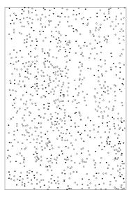
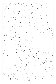
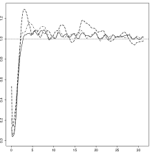
Figure 5: Left: Allogny dataset of sound oaks (circles) and splited oaks (solid points). Middle: splited oaks only. Right: non-parametric estimate of the pair correlation function for all trees (solid curve), the sound oaks (dotted-dashed curve), and the splited oaks (dashed curve).

We apply our model to this dataset where $X$ represents the splited oaks and $Y$ is the unmarked point pattern composed of the splited and the sound oaks. In this application, the inclusion probabilities given by $\Pi$ have a natural interpretation in terms of unobserved environmental conditions that locally favor frost shake. Specifically, following the procedure explained in Section 4.2, we fit a parametric model to $\Pi$ by the composite likelihood method. We are in particularly interested here by the conditional simulation of $\Pi$ given the observation of the sound oaks and the splited oaks.

Both models presented in Sections 3.2-3.3 can be considered for $\Pi$. However we think that a Boolean model is too simple to explain the clustering behaviour of splited trees and we therefore assume that $-\log\Pi$ is a squared stationary and isotropic Gaussian process given by (14) with $k=1$ and $R_{0}$ being a Whittle-Matérn correlation function with shape parameter $\nu>0$ and scale parameter $s>0$ (see Lavancier et al. (2015)). The estimate of $q$ is $\hat{q}=256/910=0.28$ whereby (15) gives $\hat{\kappa}=11.8$, and by maximizing (27) using a grid of values for $\nu$ and substituting $q$ by $\hat{q}$, we obtain $\hat{s}=7.8$ and $\hat{\nu}=0.5$, in which case $R_{0}$ becomes the exponential correlation function. The goodness of fit is assessed by comparing non-parametric estimates of the $K$, $F$, $G$, and $J$ functions (see e.g. Møller and Waagepetersen (2004)) for the splited oaks with $95\%$ pointwise envelopes of the same functions obtained from simulations of the fitted model. Here, in accordance with our inference procedure, the simulation of new splited oaks is done conditionally on the tree locations, meaning that only $\Pi$ is simulated. The results are reported in Figure 6. Furthermore, the same comparison is done for the sound oaks in Figure 7. Figures 6-7 show that the goodness of fit is acceptable.

Figure 6: From left to right non-parametric estimates of the $K$, $F$, $G$, and $J$ functions for the splited oaks (solid lines) along with simulated $95\%$ pointwise envelopes obtained under the fitted model of Section 5.1 (dashed lines).

Figure 7: From left to right non-parametric estimates of the $K$, $F$, $G$, and $J$ functions for the sound oaks (solid lines) along with simulated $95\%$ pointwise envelopes obtained under the fitted model of Section 5.1 (dashed lines).

Next, assuming $\Pi$ follows the fitted model, we simulate $\Pi$ conditional on the splited oaks and the sound oaks, using the two steps procedure detailed in Section 4.1. Figure 8 shows two such realizations of $\Pi$ and an approximation of the conditional expectation obtained from the average over 100 independent realizations of $\Pi$. The white and lighter areas in these grayscale plots correspond to regions where frost shake seems unlikely to happen. The two simulated realizations illustrate the ‘roughness’ of $\Pi$ due to the underlying exponential covariance function. As expected, the conditional expectation of $\Pi$ is large in the neighborhoods of splited oaks.

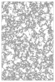
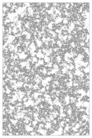
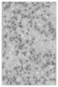
Figure 8: Typical simulations (left and middle) and approximated expectation (right) of $\Pi$ under the fitted model of Section 5.1, conditional on the splited oaks and the sound oaks.

5.2 Ponderosa dataset

Figure 9 shows the location of 108 ponderosa pine trees in a $120\times 120$m area of the Klamath National Forest in Northern California. This dataset is available in the spatstat library and was studied in Getis and Franklin (1987). By a descriptive second-order analysis, the authors identified different types of clustering between the trees, depending on the scale. In particular they noticed that “there are clusters of points and an apparent inhibition effect”.

Figure 9: Left: Ponderosa dataset. Right: Non-parametric estimate of its pair correlation function.

We fit our model to this dataset where $Y$ is assumed to be a DPP and $\Pi$ to follow (14) with a Gaussian covariance function or (17) where $\Delta_{0}$ is deterministic. Three parametric families of kernels were considered for the DPP: the Gaussian covariance functions, the Whittle-Matérn covariance functions (see Lavancier et al. (2015)), and the Bessel-type covariance functions (see Biscio and Lavancier (2015)). These covariance functions depend on the intensity $\rho_{Y}$ (which is equal to the variance), on a scale parameter $\alpha$ and for the Whittle-Matérn and Bessel-type covariance functions on an extra shape parameter, denoted $\nu$ and $\sigma$, respectively. The Gaussian kernels family is in fact a limiting case of the two others families when $\nu$, respectively $\sigma$, tends to infinity. It is well known that the identification of both $\alpha$ and $\nu$ (respectively $\sigma$) is difficult, even when $Y$ is fully observed and not thinned by $\Pi$. To estimate all parameters, we use a minimum contrast method as explained in Section 4.2 for different values of $\nu$ (respectively $\sigma$) on a grid and then choose the parameters giving the minimal value of the contrast function.

Among all fitted six models, we selected the one associated to the minimal value of the contrast function based on the pair correlation function, cf. (29). The best fit was then obtained for $Y$ being the DPP with a Gaussian covariance function and $\Pi$ the Boolean model, where the minimum contrast procedure together with (18)-(19) give the estimates $\hat{\alpha}=5.26$ (with $\alpha$ being the scale parameter of the Gaussian covariance function), $\hat{q}=0.74$, and $\hat{\Delta}_{0}=23.14$. Further, $\hat{q}=0.74$ together with the natural estimate $\hat{\rho}_{X}=108/(120)^{2}=0.0075$ give $\hat{\rho}_{Y}=\hat{\rho}_{X}/\hat{q}=0.01$. When trying to improve the estimation of the selected model by the combination method based of the $g$ and $K$ functions (described at the end of Section 4.2), the best weight was (1,0), thus confirming the choice of the contrast function based on $g$ for this model. The goodness of fit is assessed by comparing the non-parametric estimates of the $K$, $F$, $G$, and $J$ functions based on the data with $95\%$ pointwise envelopes of the same functions obtained from simulations of the fitted model. The result is shown in Figure 10 where the fitted model appears to provide a good fit.

Figure 10: From left to right non-parametric estimation of the $K$, $F$, $G$, and $J$ functions for the Ponderosa dataset (solid lines) along with simulated $95\%$ pointwise envelopes under the fitted model of Section 5.2 (dashed lines).

Acknowledgment

Supported by the Danish Council for Independent Research — Natural Sciences, grant 12-124675, ”Mathematical and Statistical Analysis of Spatial Data”, and by the ”Centre for Stochastic Geometry and Advanced Bioimaging”, funded by grant 8721 from the Villum Foundation.

References

- Andersen and Hahn (2015) Andersen, I. T. and U. Hahn (2015). Matérn thinned Cox processes. In preparation.
- Baddeley and Turner (2005) Baddeley, A. and R. Turner (2005). Spatstat: an R package for analyzing spatial point patterns. Journal of Statistical Software 12(6), 1–42. URL: www.jstatsoft.org, ISSN: 1548-7660.
- Biscio and Lavancier (2015) Biscio, C. A. N. and F. Lavancier (2015). Quantifying repulsiveness of determinantal point processes. Bernoulli. To appear.
- Chiu et al. (2013) Chiu, S. N., D. Stoyan, W. S. Kendall, and J. Mecke (2013). Stochastic Geometry and Its Applications (Third ed.). Wiley, Chichester.
- Cox (1972) Cox, D. R. (1972). The statistical analysis of dependencies in point processes. In P. A. W. Lewis (Ed.), Stochastic Point Processes, pp. 55–66. Wiley, New York.
- Cressie (1993) Cressie, N. A. C. (1993). Statistics for Spatial Data (Second ed.). Wiley, New York.
- Daley and Vere-Jones (2003) Daley, D. J. and D. Vere-Jones (2003). An Introduction to the Theory of Point Processes. Volume I: Elementary Theory and Methods (Second ed.). Springer-Verlag, New York.
- Diggle (2003) Diggle, P. (2003). Statistical Analysis of Spatial Point Patterns (Second ed.). London: Hodder Arnold.
- Getis and Franklin (1987) Getis, A. and J. Franklin (1987). Second-order neighborhood analysis of mapped point patterns. Ecology 68, 473–477.
- Goldstein et al. (2015) Goldstein, J., M. Haran, I. Simeonov, J. Fricks, and F. Chiaromonte (2015). An attraction-repulsion point process model for respiratory syncytial virus infections. Biometrics. To appear.
- Goreaud and Pélissier (2003) Goreaud, F. and R. Pélissier (2003). Avoiding misinterpretation of biotic interactions with the intertype K12-function: population independence vs. random labelling hypotheses. Journal of Vegetation Science 14, 681–692.
- Illian et al. (2008) Illian, J., A. Penttinen, H. Stoyan, and D. Stoyan (2008). Statistical Analysis and Modelling of Spatial Point Patterns. John Wiley and Sons, Chichester.
- Kautz et al. (2011) Kautz, M., U. Berger, D. Stoyan, J. Vogt, N. I. Khan, K. Diele, U. Saint-Paul, T. Rriet, and V. N. Nam (2011). Desynchronizing effects of lightning strike disturbances on cyclic forest dynamics in mangrove plantations. Aquatic Botany 95, 173–181.
- Kendall and Møller (2000) Kendall, W. S. and J. Møller (2000). Perfect simulation using dominating processes on ordered spaces, with application to locally stable point processes. Advances in Applied Probability 32, 844–865.
- Kingman (1993) Kingman, J. F. C. (1993). Poisson Processes. Oxford: Clarendon Press.
- Lantuéjoul (2002) Lantuéjoul, C. (2002). Geostatistical Simulation: Models and Algorithms. Number 1139. Springer Science & Business Media, Berlin.
- Lavancier et al. (2015) Lavancier, F., J. Møller, and E. Rubak (2015). Determinantal point process models and statistical inference. Journal of the Royal Statistical Society: Series B (Statistical Methodology). To appear.
- Lavancier and Rochet (2015) Lavancier, F. and P. Rochet (2015). A general procedure to combine estimators. Computational Statistics and Data Analysis. To appear.
- Lieshout (2000) Lieshout, M. N. M. v. (2000). Markov Point Processes and Their Applications. Imperial College Press, London.
- Macchi (1975) Macchi, O. (1975). The coincidence approach to stochastic point processes. Advances in Applied Probability 7, 83–122.
- Matérn (1986) Matérn, B. (1986). Spatial Variation. Lecture Notes in Statistics 36, Springer-Verlag, Berlin.
- McCullagh and Møller (2006) McCullagh, P. and J. Møller (2006). The permanental process. Advances in Applied Probability 38, 873–888.
- Molchanov (1997) Molchanov, I. (1997). Statistics of the Boolean Model for Practitioners and Mathematicians. Wiley, Chichester.
- Møller et al. (2010) Møller, J., M. L. Huber, and R. L. Wolpert (2010). Perfect simulation and moment properties for the Matérn type III process. Stochastic Processes and their Applications 120, 2142–2158.
- Møller and Waagepetersen (2004) Møller, J. and R. P. Waagepetersen (2004). Statistical Inference and Simulation for Spatial Point Processes. Boca Raton: Chapman and Hall/CRC.
- Møller and Waagepetersen (2007) Møller, J. and R. P. Waagepetersen (2007). Modern spatial point process modelling and inference (with discussion). Scandinavian Journal of Statistics 34, 643–711.
- Pélissier and Goreaud (2015) Pélissier, R. and F. Goreaud (2015). ads package for R: A fast unbiased implementation of the -function family for studying spatial point patterns in irregular-shaped sampling windows. Journal of Statistical Software 63, 1–18.
- R Core Team (2014) R Core Team (2014). R: A Language and Environment for Statistical Computing. Vienna, Austria: R Foundation for Statistical Computing.
- Ruelle (1969) Ruelle, D. (1969). Statistical Mechanics: Rigorous Results. W.A. Benjamin, Reading, Massachusetts.
- Schlather et al. (2015) Schlather, M., A. Malinowski, M. Oesting, D. Boecker, K. Strokorb, S. Engelke, J. Martini, F. Ballani, P. J. Menck, S. Gross, U. Ober, K. Burmeister, J. Manitz, P. Ribeiro, R. Singleton, B. Pfaff, and R Core Team (2015). RandomFields: Simulation and Analysis of Random Fields. R package version 3.0.55.
- Stoyan (1979) Stoyan, D. (1979). Interrupted point processes. Biometrical Journal 21, 607–610.