Phase-coherent mapping of gravitational-wave backgrounds using ground-based
laser interferometers

Abstract

We extend the formalisms developed in Gair et al. Gair et al. (2014) and Cornish and van Haasteren Cornish and van Haasteren (2014) to create maps of gravitational-wave backgrounds using a network of ground-based laser interferometers. We show that in contrast to pulsar timing arrays, which are insensitive to half of the gravitational-wave sky (the curl modes), a network of ground-based interferometers is sensitive to both the gradient and curl components of the background. The spatial separation of a network of interferometers, or of a single interferometer at different times during its rotational and orbital motion around the Sun, allows for recovery of both components. We derive expressions for the response functions of a laser interferometer in the small-antenna limit, and use these expressions to calculate the overlap reduction function for a pair of interferometers. We also construct maximum-likelihood estimates of the $+$ and $\times$-polarization modes of the gravitational-wave sky in terms of the response matrix for a network of ground-based interferometers, evaluated at discrete times during Earth’s rotational and orbital motion around the Sun. We demonstrate the feasibility of this approach for some simple simulated backgrounds (a single point source and spatially-extended distributions having only grad or curl components), calculating maximum-likelihood sky maps and uncertainty maps based on the (pseudo)inverse of the response matrix. The distinction between this approach and standard methods for mapping gravitational-wave power is also discussed.

I Introduction

Searches for anisotropic gravitational-wave backgrounds have typically been formulated in terms of the distribution of gravitational-wave power on the sky (see, e.g., Allen and Ottewill (1997); Cornish (2001); Mitra et al. (2008); Thrane et al. (2009); Abadie et al. (2011); Mingarelli et al. (2013); Taylor and Gair (2013)). The basic idea underlying these approaches is to use to cross-correlation measurements from two or more detectors to estimate the power in the gravitational-wave background as a function of sky position. For a network of ground-based laser interferometers like LIGO The LIGO Scientific Collaboration et al. (2015), Virgo Acernese et al. (2015), etc., or space-based interferometers like LISA Danzmann and LISA Study (1996), eLISA Amaro-Seoane et al. (2012); Amaro-Seoane et al. (2013) or BBO Phinney et al. (2004), the motion of the detectors modulates the correlated gravitational-wave signal at harmonics of the Earth’s daily rotational motion, or the spacecrafts’ yearly orbital motion around the Sun. The time-varying signal carries information about the multipole moments characterizing the anisotropic distribution of power, which can be estimated using, e.g., maximum-likelihood methods Thrane et al. (2009).

Recent papers by Gair et al. Gair et al. (2014) and Cornish and van Haasteren Cornish and van Haasteren (2014) describe an alternative approach for mapping the gravitational-wave sky, which can be used to recover both the amplitude and phase of the gravitational-wave signal at each sky position. The analysis in Cornish and van Haasteren (2014) is cast in terms of the traditional plus and cross polarization components $\{h_{+}(f,\hat{k})$, $h_{\times}(f,\hat{k})\}$, while in Gair et al. (2014) the metric perturbations are decomposed in terms of spin-weighted or tensor (gradient and curl) spherical harmonics $\{Y^{G}_{(lm)ab}(\hat{k})$, $Y^{C}_{(lm)ab}(\hat{k})\}$. This latter decomposition is similar to that used to characterize the polarization of the cosmic microwave background Kamionkowski et al. (1997), taking into account the symmetric, transverse-traceless nature of the metric perturbations $h_{ab}(f,\hat{k})$.

Although the formalisms introduced in Gair et al. (2014); Cornish and van Haasteren (2014) are general, they were applied specifically to the case of gravitational-wave searches using pulsar timing arrays. In contrast to the case of ground-based interferometers on a rotating, orbiting Earth or the orbiting LISA/eLISA spacecraft, a pulsar timing array operates effectively as a static galactic-scale gravitational-wave detector Foster and Backer (1990), with each Earth-pulsar line-of-sight being the equivalent of a one-way, one-arm interferometer with a common endpoint at the solar system barycentre (SSB). This is because the frequency range for pulsar timing measurements is such that the displacement of a detector on Earth from the SSB is much smaller than the wavelength of the relevant gravitational waves, and hence the detector effectively resides at the SSB. In addition, the times of arrival of the pulses from a given set of pulsars at a radio telescope are typically converted to arrival times at the SSB, which is a fixed origin. A consequence of the static nature of pulsar-timing measurements is that a pulsar timing array will never be able to observe half of the gravitational-wave sky regardless of how many pulsars are included in the array Gair et al. (2014). In particular, the response of a pulsar timing array to curl modes is identically zero, as the gravitational contribution of such modes to the timing residual equals zero when integrated over the sky.

In this paper, we extend the formalisms developed in Gair et al. (2014); Cornish and van Haasteren (2014) to the case of ground-based interferometers like LIGO, Virgo, etc. For simplicity we work in the small-antenna (or long-wavelength) limit, which is appropriate for such detectors. We show that in contrast to pulsar timing arrays, a network of ground-based interferometers is sensitive to both the gradient and curl modes of the background. The fact that the spatial separation of the detectors is the same order or greater than the radiation wavelength is sufficient to allow for recovery of both types of mode. We demonstrate this by: (i) explicitly deriving analytic expressions for the gradient and curl response functions of a laser interferometer, and (ii) constructing maximum-likelihood estimates of the gravitational-wave sky for different types of simulated backgrounds. The reconstruction of the sky maps is based on singular value decomposition (SVD) of the whitened response matrix $\bar{\mathbf{R}}=\bar{\mathbf{U}}\bar{\bm{\Sigma}}\bar{\mathbf{V}}^{\dagger}$, which maps the modes of the gravitational-wave background to the response of the individual interferometers, evaluated at discrete times during Earth’s rotational and orbital motion around the sun. The columns of $\bar{\mathbf{U}}$ and $\bar{\mathbf{V}}$ corresponding to the non-zero singular values of $\bar{\bm{\Sigma}}$ have the interpretation of response range vectors and sky map basis vectors, in terms of which the measured response and the maximum-likelihood sky map can be written as linear combinations Cornish and van Haasteren (2014). The recovered sky maps can be calculated in terms of either a pixel-based parametrisation, $\{h_{+}(f,\hat{k}_{n}),h_{\times}(f,\hat{k}_{n})\}$, where $n$ labels the pixels on the sky, or in terms of the gradient and curl spherical harmonic components $\{a^{G}_{(lm)}(f)$, $a^{C}_{(lm)}(f)\}$, where $(lm)$ labels the various multipole modes, up to some maximum value $l_{\rm max}$.

The organization of the rest of the paper is as follows: In Sec. II, we summarize key formulae related to the tensor spherical harmonic decomposition approach described in Gair et al. (2014). We derive, in Sec. III, analytic expressions for the gradient and curl response functions of a laser interferometer in the small-antenna limit. (Details of the derivation are given in Appendix A.) In Sec. IV, we show that we can recover the standard overlap reduction functions using the analytic expressions for the response functions derived in Sec. III, and in Sec. V we compare the effects of Earth’s rotational and orbital motion on the sky reconstruction. We describe the map-making formalism in Sec. VI and demonstrate that a network of ground-based inteferometers can recover both the grad and curl components of a gravitational-wave background, by constructing maximum-likelihood sky maps for some simple simulations. We conclude in Sec. VII with a brief summary and discussion of the results, listing a few modifications that might be needed in order to apply this formalism to real data.

II Brief review of tensor spherical harmonic decomposition

For completeness, we summarize in this section some key formulae from the tensor spherical harmonic decomposition method described in Gair et al. (2014). Interested readers are referred to that paper for more details.

Any transverse-traceless tensor field on the sky can be decomposed as a superposition of gradients and curls of spherical harmonics:

$$Y^{G}_{(lm)ab}(\hat{k}) =N_{l}\left[Y_{(lm);ab}(\hat{k})-\frac{1}{2}g_{ab}Y_{(lm);c}{}^{c}(\hat{k})\right]\,,$$ (1)

$$Y^{C}_{(lm)ab}(\hat{k}) =\frac{N_{l}}{2}\left[Y_{(lm);ac}(\hat{k})\epsilon^{c}{}_{b}+Y_{(lm);bc}(\hat{k})\epsilon^{c}{}_{a}\right]\,,$$

where semi-colon denotes covariant derivative, $g_{ab}$ is the metric tensor on the sphere, $\epsilon_{ab}$ is the Levi-Civita anti-symmetric tensor

$$\epsilon_{ab}=\sqrt{g}\left(\begin{array}[]{cc}0&1\\ -1&0\end{array}\right)\,,$$ (2)

and $N_{l}$ is a normalization constant

$$N_{l}=\sqrt{\frac{2(l-2)!}{(l+2)!}}\,.$$ (3)

In terms of the standard polarization tensors on the sky

$$e_{ab}^{+}(\hat{k}) =\hat{\theta}_{a}\hat{\theta}_{b}-\hat{\phi}_{a}\hat{\phi}_{b}\,,$$ (4)

$$e_{ab}^{\times}(\hat{k}) =\hat{\theta}_{a}\hat{\phi}_{b}+\hat{\phi}_{a}\hat{\theta}_{b}\,,$$

we have

$$Y^{G}_{(lm)ab}(\hat{k}) =\frac{N_{l}}{2}\left[W_{(lm)}(\hat{k})e_{ab}^{+}(\hat{k})+X_{(lm)}(\hat{k})e_{ab}^{\times}(\hat{k})\right]\,,$$ (5)

$$Y^{C}_{(lm)ab}(\hat{k}) =\frac{N_{l}}{2}\left[W_{(lm)}(\hat{k})e_{ab}^{\times}(\hat{k})-X_{(lm)}(\hat{k})e_{ab}^{+}(\hat{k})\right]\,,$$

where $W_{(lm)}(\hat{k})$ and $X_{(lm)}(\hat{k})$ can be written in terms of associated Legendre polynomials as

$$W_{(lm)}(\hat{k}) =+2\sqrt{\frac{2l+1}{4\pi}\frac{(l-m)!}{(l+m)!}}\left\{-\left(\frac{l-m^{2}}{\sin^{2}\theta}+\frac{1}{2}l(l-1)\right)P^{m}_{l}(\cos\theta)+(l+m)\frac{\cos\theta}{\sin^{2}\theta}P^{m}_{l-1}(\cos\theta)\right\}e^{im\phi}\,,$$ (6)

$$iX_{(lm)}(\hat{k}) =-2\sqrt{\frac{2l+1}{4\pi}\frac{(l-m)!}{(l+m)!}}\left\{\frac{m}{\sin^{2}\theta}\left[(l-1)\cos\theta P_{l}^{m}(\cos\theta)-(l+m)P^{m}_{l-1}(\cos\theta)\right]\right\}e^{im\phi}\,,$$ (7)

and are related to spin-2 spherical harmonics Newman and Penrose (1966); Goldberg et al. (1967) through the equation

$${}_{\pm 2}Y_{(lm)}(\hat{k})=\frac{N_{l}}{\sqrt{2}}\left[W_{(lm)}(\hat{k})\pm iX_{(lm)}(\hat{k})\right]\,.$$ (8)

In terms of the grad and curl spherical harmonics, a general gravitational-wave background can be decomposed as

$$h_{ab}(t,\vec{x})=\int_{-\infty}^{\infty}{\rm d}f\>\int_{S^{2}}{\rm d}^{2}\Omega_{\hat{k}}\>h_{ab}(f,\hat{k})e^{i2\pi f(t-\hat{k}\cdot\vec{x}/c)}\,,$$ (9)

where

$$h_{ab}(f,\hat{k})=\sum_{l=2}^{\infty}\sum_{m=-l}^{l}\left[a^{G}_{(lm)}(f)Y^{G}_{(lm)ab}(\hat{k})+a^{C}_{(lm)}(f)Y^{C}_{(lm)ab}(\hat{k})\right]\,.$$ (10)

The mode functions $a^{G}_{(lm)}(f)$, $a^{C}_{(lm)}(f)$ are related to the more traditional $+$ and $\times$ polarisation components $h_{+}(f,\hat{k})$, $h_{\times}(f,\hat{k})$ defined by

$$h_{ab}(f,\hat{k})\!=\!h_{+}(f,\hat{k})e^{+}_{ab}(\hat{k})+h_{\times}(f,\hat{k})e^{\times}_{ab}(\hat{k})\,,$$ (11)

via

$$h_{+}(f,\hat{k}) =\!\sum_{(lm)}\!\frac{N_{l}}{2}\!\left[a^{G}_{(lm)}(f)W_{(lm)}(\hat{k})-a^{C}_{(lm)}(f)X_{(lm)}(\hat{k})\right],$$ (12)

$$h_{\times}(f,\hat{k}) =\!\sum_{(lm)}\!\frac{N_{l}}{2}\!\left[a^{G}_{(lm)}(f)X_{(lm)}(\hat{k})+a^{C}_{(lm)}(f)W_{(lm)}(\hat{k})\right],$$

and

$$a^{G}_{(lm)}\!(f)\!=\!N_{l}\!\!\int_{S^{2}}\!\!\!{\rm d}^{2}\Omega_{\hat{k}}\!\left[h_{+}\!(f,\hat{k})W_{(lm)}^{*}\!(\hat{k})\!+\!h_{\times}\!(f,\hat{k})X_{(lm)}^{*}\!(\hat{k})\right],$$ (13)

$$a^{C}_{(lm)}\!(f)\!=\!N_{l}\!\!\int_{S^{2}}\!\!\!{\rm d}^{2}\Omega_{\hat{k}}\!\left[h_{\times}\!(f,\hat{k})W_{(lm)}^{*}\!(\hat{k})\!-\!h_{+}\!(f,\hat{k})X_{(lm)}^{*}\!(\hat{k})\right]\,,$$

where we use the shorthand $\sum_{(lm)}\equiv\sum_{l=2}^{\infty}\sum_{m=-l}^{l}$. Note that all the summations over $l$ start at $l=2$.

III Response function calculations

The frequency-domain response of a laser interferometer to a gravitational-wave background is given by

$$\tilde{r}(f)=\int_{S^{2}}{\rm d}^{2}\Omega_{\hat{k}}\sum_{A}R^{A}(f,\hat{k})h_{A}(f,\hat{k})\,,$$ (14)

where $A=\{+,\times\}$ and

$$R^{A}(f,\hat{k})=\frac{1}{2}e^{A}_{ab}(\hat{k})(u^{a}u^{b}-v^{a}v^{b})e^{-i2\pi f\hat{k}\cdot\vec{x}_{0}/c}\,.$$ (15)

Here $\hat{u}$, $\hat{v}$ are unit vectors along the arms of the interferometer and $\vec{x}_{0}$ is the position vector of the vertex of the interferometer at the time $t$ when the measurement is made. The above expression for $R^{A}(f,\hat{k})$ is valid in the small-antenna limit, which is appropriate for ground-based interferometers like LIGO, Virgo, etc. (see e.g., Mingarelli and Sidery (2014) for this discussion in the pulsar timing context). The length of the interferometer arms do not enter the expressions for the response functions in this limit.

Alternatively, if we expand the metric perturbations in terms of the gradient and curl modes $\{a^{G}_{(lm)}(f),a^{C}_{(lm)}(f)\}$, the response can be written as

$$\tilde{r}(f)=\sum_{(lm)}\sum_{P}R^{P}_{(lm)}(f)a^{P}_{(lm)}(f)\,,$$ (16)

where $P=\{G,C\}$ and

$$R^{G}_{(lm)}(f) =\frac{N_{l}}{2}\int_{S^{2}}{\rm d}^{2}\Omega_{\hat{k}}\>\left[R^{+}(f,\hat{k})W_{(lm)}(\hat{k})+R^{\times}(f,\hat{k})X_{(lm)}(\hat{k})\right]\,,$$ (17)

$$R^{C}_{(lm)}(f) =\frac{N_{l}}{2}\int_{S^{2}}{\rm d}^{2}\Omega_{\hat{k}}\>\left[R^{\times}(f,\hat{k})W_{(lm)}(\hat{k})-R^{+}(f,\hat{k})X_{(lm)}(\hat{k})\right]\,.$$

These integrals were evaluated in Appendix D of Gair et al. (2014) for the case of a reference frame which has $\vec{x}_{0}=\vec{0}$:

$$R^{G}_{(lm)}(f)\big{|}_{\vec{x}_{0}=\vec{0}} =\delta_{l2}\,\frac{4\pi}{5}\sqrt{\frac{1}{3}}\left[Y_{2m}(\hat{u})-Y_{2m}(\hat{v})\right]\,,$$ (18)

$$R^{C}_{(lm)}(f)\big{|}_{\vec{x}_{0}=\vec{0}} =0\,.$$

Note that the curl response is identically zero in this frame, while the gradient response is independent of frequency and is non-zero only for the quadrupole components, $l=2$. These results are qualitatively similar to those for a pulsar timing array, which also have zero curl response, and a frequency-independent grad response proportional to $Y_{lm}(\hat{u})$, where $\hat{u}$ points in the direction to the pulsar. In what follows, we will use the notation

$$F_{m}(\hat{u},\hat{v})\equiv\frac{4\pi}{5}\sqrt{\frac{1}{3}}\left[Y_{2m}(\hat{u})-Y_{2m}(\hat{v})\right]$$ (19)

to denote the particular combination of spherical harmonics that appear in Eq. (18). Since only the quadrupole response is non-zero, the index $m$ on $F_{m}$ is restricted to have values $m=0,\pm 1,\pm 2$.

For a single static interferometer, there is no loss in generality in choosing a reference frame with the vertex of the interferometer located at the origin, with the response functions given as above. But for a network of interferometers attached to a rotating and orbiting Earth, such a coordinate choice is no longer possible. If an interferometer is displaced from the origin by $\vec{x}_{0}$, one can show that

$$R^{G}_{(lm)}(f)= \sum_{m^{\prime}=-2}^{2}\sum_{L=l-2}^{l+2}\sum_{M=-L}^{L}F_{m^{\prime}}(\hat{u},\hat{v})4\pi(-i)^{L}j_{L}(\alpha)Y^{*}_{LM}(\hat{x}_{0})$$ (20)

$$\times\frac{(-1)^{m^{\prime}}}{2}\sqrt{\frac{(2\cdot 2+1)(2l+1)(2L+1)}{4\pi}}\left(\begin{array}[]{ccc}2&l&L\\ -m^{\prime}&m&M\end{array}\right)\left(\begin{array}[]{ccc}2&l&L\\ 2&-2&0\end{array}\right)\left[(-1)^{l+L}+1\right]\,,$$

$$R^{C}_{(lm)}(f)= \sum_{m^{\prime}=-2}^{2}\sum_{L=l-2}^{l+2}\sum_{M=-L}^{L}F_{m^{\prime}}(\hat{u},\hat{v})4\pi(-i)^{L}j_{L}(\alpha)Y^{*}_{LM}(\hat{x}_{0})$$

$$\times\frac{(-1)^{m^{\prime}}}{2i}\sqrt{\frac{(2\cdot 2+1)(2l+1)(2L+1)}{4\pi}}\left(\begin{array}[]{ccc}2&l&L\\ -m^{\prime}&m&M\end{array}\right)\left(\begin{array}[]{ccc}2&l&L\\ 2&-2&0\end{array}\right)\left[(-1)^{l+L}-1\right]\,,$$

where $\alpha\equiv 2\pi f|\vec{x}_{0}|/c$ and $j_{L}(\alpha)$ are spherical Bessel functions of order $L$. These expressions are derived in Appendix A. The two expressions in parentheses $(\ )$ for each response function are Wigner 3-$j$ symbols (see for example Wigner (1959), Messiah (1962)). Note that, in general, the curl response is now non-zero, in contrast to the static single interferometer case. In addition, both response functions depend on frequency via the quantity $\alpha$, which has the physical interpretation of being $2\pi$ times the number of radiation wavelengths between the origin and the vertex of the interferometer. Since the coordinate system for the response functions in (18) was not chosen in any particular orientation relative to the unit vectors $\hat{u}$ and $\hat{v}$, Eqs. (20) are valid in an arbitrary translated and rotated coordinate system, provided we use the angles for $\hat{u}$, $\hat{v}$, and $\hat{x}_{0}$ as calculated in the rotated frame.

IV Recovery of standard overlap reduction functions

Given the above expressions for $R^{P}_{(lm)}(f)$ one can calculate the overlap reduction function $\Gamma_{12}(f)$ for a pair of interferometers for gravitational-wave backgrounds having different statistical properties. For example, for a statistically isotropic background with $C^{GG}_{l}=C^{CC}_{l}\equiv C_{l}$ and $C^{GC}_{l}=0=C^{CG}_{l}$, it was shown in Gair et al. (2014) that

$$\Gamma_{12}(f)=\sum_{l=2}^{\infty}C_{l}\Gamma_{12,l}(f)\,,$$ (21)

where

$$\Gamma_{12,l}(f)=\sum_{m=-l}^{l}R^{P}_{1(lm)}(f)R^{P*}_{2(lm)}(f)\,.$$ (22)

This is most-easily evaluated in a reference frame in which the vertex of one interferometer is located at the origin, and the vertex of the second interferometer is located along the $z$-axis of this frame. This so-called computational frame is related to the cosmic reference frame located at the solar system barycentre via a translation by the position vector $\vec{x}_{1}$ and a rotation ${\cal R}\equiv{\cal R}_{y}(\theta_{0}){\cal R}_{z}(\phi_{0})$ such that $\Delta\vec{x}\equiv\vec{x}_{2}-\vec{x}_{1}$ is directed along the $z$-axis. (Here $(\theta_{0},\phi_{0})$ are the polar and azimuthal angles of $\Delta\vec{x}$ with respect to the cosmic frame.) In the computational frame

$$R^{P}_{1(lm)}(f)=\delta^{PG}\delta_{l2}\,F_{m}({\cal R}\hat{u}_{1},{\cal R}\hat{v}_{1})\,,$$ (23)

where the arguments of $F_{m}$ are the polar and azimuthal angles of $\hat{u}_{1}$ and $\hat{v}_{1}$ with respect to the computational frame. This form for $R^{P}_{1(lm)}(f)$ implies

$$\Gamma_{12,l}(f)=\delta_{l2}\sum_{m=-2}^{2}F_{m}({\cal R}\hat{u}_{1},{\cal R}\hat{v}_{1})R^{G*}_{2(2m)}(f)\,,$$ (24)

which in turn implies

$$\Gamma_{12}(f) =C_{2}\,\Gamma_{12,2}(f)$$ (25)

$$=C_{2}\sum_{m=-2}^{2}F_{m}({\cal R}\hat{u}_{1},{\cal R}\hat{v}_{1})R^{G*}_{2(2m)}(f)\,.$$

Thus, the only non-zero contribution to the overlap reduction function comes from the quadrupole gradient terms. Using Eq. (20), it follows that

$$R^{G}_{2(2m)}(f)=F_{m}({\cal R}\hat{u}_{2},{\cal R}\hat{v}_{2})\bigg{[}j_{0}(\alpha) +(-1)^{m+1}(2\cdot 2+1)^{2}\left(\begin{array}[]{ccc}2&2&2\\ -m&m&0\end{array}\right)\left(\begin{array}[]{ccc}2&2&2\\ 2&-2&0\end{array}\right)j_{2}(\alpha)$$ (30)

$$+(-1)^{m}(2\cdot 2+1)(2\cdot 4+1)\left(\begin{array}[]{ccc}2&2&4\\ -m&m&0\end{array}\right)\left(\begin{array}[]{ccc}2&2&4\\ 2&-2&0\end{array}\right)j_{4}(\alpha)\bigg{]}\,,$$ (35)

where $\alpha\equiv 2\pi f|\Delta\vec{x}|/c$. Thus,

$$\Gamma_{12}(f)=C_{2}\left[Aj_{0}(\alpha)+Bj_{2}(\alpha)+Cj_{4}(\alpha)\right]\,,$$ (36)

where

$$A =\sum_{m=-2}^{2}F_{m}({\cal R}\hat{u}_{1},{\cal R}\hat{v}_{1})F^{*}_{m}({\cal R}\hat{u}_{2},{\cal R}\hat{v}_{2})\,,$$ (37)

$$B =\sum_{m=-2}^{2}F_{m}({\cal R}\hat{u}_{1},{\cal R}\hat{v}_{1})F^{*}_{m}({\cal R}\hat{u}_{2},{\cal R}\hat{v}_{2})(-1)^{m+1}(2\cdot 2+1)^{2}\left(\begin{array}[]{ccc}2&2&2\\ -m&m&0\end{array}\right)\left(\begin{array}[]{ccc}2&2&2\\ 2&-2&0\end{array}\right)\,,$$

$$=\frac{5}{7}\sum_{m=-2}^{2}F_{m}({\cal R}\hat{u}_{1},{\cal R}\hat{v}_{1})F^{*}_{m}({\cal R}\hat{u}_{2},{\cal R}\hat{v}_{2})(-1)^{2m+1}(m^{2}-2)\,,$$

$$C =\sum_{m=-2}^{2}F_{m}({\cal R}\hat{u}_{1},{\cal R}\hat{v}_{1})F^{*}_{m}({\cal R}\hat{u}_{2},{\cal R}\hat{v}_{2})(-1)^{m}(2\cdot 2+1)(2\cdot 4+1)\left(\begin{array}[]{ccc}2&2&4\\ -m&m&0\end{array}\right)\left(\begin{array}[]{ccc}2&2&4\\ 2&-2&0\end{array}\right)\,,$$

$$=\frac{12}{7}\sum_{m=-2}^{2}F_{m}({\cal R}\hat{u}_{1},{\cal R}\hat{v}_{1})F^{*}_{m}({\cal R}\hat{u}_{2},{\cal R}\hat{v}_{2})\frac{(-1)^{m}}{(2-m)!(2+m)!}\,.$$

Here we have used the definition of the Wigner 3-$j$ sycalol to simplify the expressions for $B$ and $C$.

For an unpolarised, isotropic and uncorrelated background, the above expression for $\Gamma_{12}(f)$ in terms of spherical Bessel functions is similar in form to expressions for the overlap reduction function in Refs. Flanagan (1993) and Allen and Romano (1999). The difference is that in those papers the expansion is in terms of $j_{0}(\alpha)$, $j_{1}(\alpha)/\alpha$, and $j_{2}(\alpha)/\alpha^{2}$, while the above expansion is in terms of $j_{0}(\alpha)$, $j_{2}(\alpha)$, and $j_{4}(\alpha)$. These two expansions can be related using the recurrence relation

$$j_{l+1}(\alpha)=\frac{2l+1}{\alpha}\,j_{l}(\alpha)-j_{l-1}(\alpha)\,,$$ (38)

for which

$$\Gamma_{12}(f)=C_{2}\bigg{[}(A-B+C)\,j_{0}(\alpha)\\ +(3B-10C)\,\frac{j_{1}(\alpha)}{\alpha}+35C\,\frac{j_{2}(\alpha)}{\alpha^{2}}\bigg{]}\,.$$ (39)

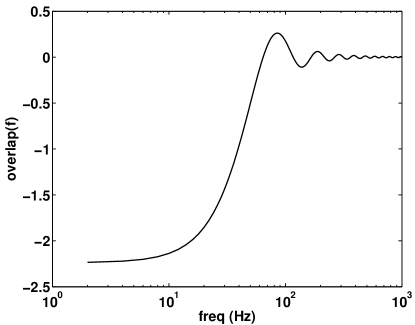
A plot of the corresponding overlap reduction function for an unpolarised statistically isotropic background is shown in Fig. 1 for the LIGO Hanford-LIGO Livingston detector pair.

Figure 1: Overlap reduction function $\Gamma_{12}(f)$ for an unpolarized statistically isotropic background for the LIGO Hanford-LIGO Livingston detector pair, plotted on a logarithmic frequency axis.

V Rotational and orbital motion

As mentioned in Sec. I, previous analyses for anisotropic stochastic backgrounds using ground-based interferometers have been formulated in terms of the distribution of gravitational-wave power on the sky Allen and Ottewill (1997); Cornish (2001); Mitra et al. (2008); Thrane et al. (2009); Abadie et al. (2011); Mingarelli et al. (2013); Taylor and Gair (2013). In addition, these approaches typically use cross-correlation measurements between pairs of detectors as the input data. As such, these analyses are insensitive to the phase of the gravitational-wave background at different spatial locations. Recall that the position-dependent phase information appears explicitly in the Fourier components of the metric perturbations, $h_{ab}(f,\hat{k})e^{-i2\pi f\hat{k}\cdot\vec{x}/c}$ (cf. Eq. (9)). It also appears in the response functions $R^{A}(f,\hat{k})$ and $R^{P}_{(lm)}(f)$, cf. Eqs. (15) and (20), where $\vec{x}_{0}$ is the location of the detector at the time $t$ at which the measurement is made. For cross-correlation measurements between a pair of detectors, the correlated response depends on the location of the detectors $\vec{x}_{1}$ and $\vec{x}_{2}$ only via their difference $\Delta\vec{x}\equiv\vec{x}_{2}-\vec{x}_{1}$, which is independent of choice of origin. Thus, the correlated response repeats after one sidereal day of observation. This means that the orbital motion of the Earth is effectively irrelevant for such analyses; only the rotational motion counts. In fact, one can fold several days of observed data to a single sidereal day, and perform the analysis on the folded data Ain et al. (2015). This has obvious benefits in regards to the reduction of data volume and the computational cost of the analysis.

In contrast, the goal of our analysis is to recover both the amplitude and phase of the gravitational-wave background at each point on the sky, based on a likelihood function that is not tied to cross-correlated data. As we shall see below, for such an analysis, the spatial locations of the detectors are as important as their relative orientations. Since our detectors are ground-based interferometers that orbit the Sun with the Earth, it is natural to reference our response functions and reconstructed sky maps back to the SSB. As such, we will take the origin of coordinates for our calculations to be the SSB. The detector locations are thus referenced from there.

Due to the Earth’s rotational and orbital motion around the Sun, a single interferometer actually defines a set of virtual interferometers located along a quasi-circular ring $1~{}{\rm AU}$ from the SSB. The Doppler shift in the observed frequency due to Earth’s velocity with respect to the SSB is not important for searches for broad-band gravitational-wave backgrounds, since $v/c\sim 10^{-4}$ introduces frequency shifts of at most $\delta f\sim{\rm few}\times 10^{-1}~{}{\rm Hz}$ in the frequency band relevant for ground-based interferometers. Thus, the rotational and orbital motion of the Earth synthesizes a set of static virtual interferometers, each observing the gravitational-wave background from a different spatial location and with a different orientation.

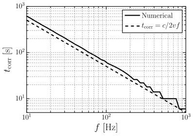
To compare the effects of rotational and orbital motion, we calculate the time-scale over which measurements made by different virtual interferometers are correlated. The relevant quantity is $\alpha=2\pi f|\Delta\vec{x}|/c$, which appears in expressions for the overlap reduction function $\Gamma_{12}(f)$, e.g. (36). But here $\Delta\vec{x}\equiv\vec{x}_{0}(t_{2})-\vec{x}_{0}(t_{1})$ is the spatial separation between the vertices of two virtual interferometers, defined by the vertex of a single (real) interferometer at times $t_{1}$ and $t_{2}$; and $f$ is the frequency of a gravitational wave. The above relation can be turned into a correlation time-scale by writing $|\Delta\vec{x}|=v\Delta t$, where $v$ is the average speed of the interferometer (due to Earth’s rotational or orbital motion) over the time interval $\Delta t\equiv t_{2}-t_{1}$, and then finding that value of $\Delta t$ for which $\alpha=\pi$:

$$t_{\rm corr}=\frac{c}{2vf}\,.$$ (40)

This corresponds to a spatial separation $|\Delta\vec{x}|=\lambda/2$, where $\lambda=c/f$ is the wavelength of the gravitational wave. For durations $\Delta t\lesssim t_{\rm corr}$, measurements taken by the two virtual interferometers are correlated; for durations $\Delta t\gtrsim t_{\rm corr}$, the measurements are uncorrelated with one another. This is justified by noting that two detectors will (on-average) be driven in coincidence by a gravitational wave propagating along their separation vector whenever its wavelength is more than twice the separation between the detectors. This argument Allen and Romano (1999) provides a rough lower bound on the decorrelation timescale of the detectors, which will actually be slightly larger since we must average over all propagation directions of the gravitational waves when considering a stochastic background.

For a gravitational wave with frequency $f=100~{}{\rm Hz}$ ($\lambda=3\times 10^{6}~{}{\rm m}$) and $v=2\pi R_{E}/(1~{}{\rm day})\approx 500~{}{\rm m/s}$, which is relevant for Earth’s daily rotational motion, we find

$$t_{\rm corr}\approx 3000~{}{\rm s}\quad({\rm rotational\ motion})\,.$$ (41)

For $v=2\pi R_{ES}/(1~{}{\rm yr})\approx 3\times 10^{4}~{}{\rm m/s}$, which is relevant for Earth’s yearly orbital motion, we find

$$t_{\rm corr}\approx 50~{}{\rm s}\quad({\rm orbital\ motion})\,.$$ (42)

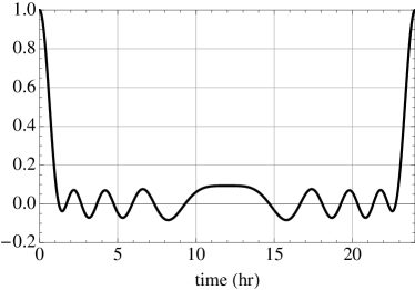
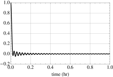
Figure 2 is the overlap reduction function $\Gamma_{12}(f)$ for an unpolarized isotropic background, evaluated at $f=100~{}{\rm Hz}$, for two virtual interferometers as a function of time. The left panel is for a set of virtual interferometers synthesized by the daily rotation of a detector positioned at the Earth’s equator, with no orbital motion. One can see that the detector decorrelates on a timescale of $\sim 1$ hour, and recorrelates after $24$ hours whenever it returns to its starting position. If we switch off daily rotation and synthesize a set of virtual interferometers from the orbital motion of the Earth around the Sun, then we get the overlap reduction function in the right panel. Since the orbital velocity of the Earth around the Sun is much larger than the velocity of a detector on the surface of the Earth, the virtual interferometers build up a larger separation baseline on a shorter timescale. Hence the overlap reduction function goes to zero much more rapidly in this case and will only recorrelate after $1$ year.

Figure 2: Overlap reduction function at $f=100~{}{\rm Hz}$ for two virtual interferometers as a function of time. The left-hand plot is for a set of virtual interferometers located on Earth’s equator, associated with Earth’s daily rotational motion. The virtual interferometers have one arm pointing North and the other pointing East. There is no orbital motion for this case, as the center of the Earth is fixed at the SSB. The right-hand plot is for a set of virtual interferometers at $1~{}{\rm AU}$ from the SSB, associated with Earth’s yearly orbital motion. There is no rotational motion for this case, as the interferometers are located at the center of the Earth in its orbit around the Sun, with the orientation of the interferometer arms unchanged by the orbital motion.

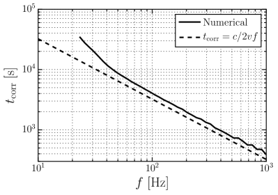
We investigate this decorrelation timescale by numerically computing the overlap reduction functions for daily rotation and orbital motion at a variety of gravitational-wave frequencies. The times at which the detectors first decorrelate are shown in Fig. 3, with the lower bounds given by Eq. (40). The decorrelation timescale does indeed obey a simple $1/f$ scaling, and at $100$ Hz the timescale for daily rotation and orbital motion are actually $\sim 67~{}{\rm min}\ (=4020~{}{\rm s})$ and $60~{}{\rm s}$, respectively. Therefore orbital motion of the Earth around the Sun will rapidly synthesize a large network of independent virtual interferometers from the motion of a single detector, with a resolving power that increases on a relatively short timescale.

Figure 3: Analysis of Fig. 2 repeated for $10\leq f\leq 1000$ Hz. The plots show the first time the overlap reduction function between virtual interferometers goes to zero for daily rotation (left panel) and orbital motion (right panel). The solid line in the left panel does not extend fully to $10$ Hz since the overlap reduction function does not go to zero at low frequencies. A rough indication of when the overlap reduction function should go to zero is given by considering that a pair of detectors should be driven in coincidence by a passing gravitational wave when the wavelength is more than twice the separation between the detectors. This defines a lower bound on the decorrelation timescale of the virtual interferometers, shown by a dashed line.

VI Map making

In this section, we extend the map-making formalism of Gair et al. (2014); Cornish and van Haasteren (2014) to data taken by a network of ground-based interferometers. The key observation is that the time-dependent ground-based interferometer analysis can be mapped to a static PTA-like analysis, for a set of static virtual interferometers in a quasi-circular ring 1 AU from the SSB. Unlike the static PTA analysis Gair et al. (2014); Cornish and van Haasteren (2014), the virtual interferometers are not all centered at the same location, but see the sky from different locations due to the Earth’s rotational and orbital motion. This allows for recovery of both the grad and curl components of the background, as discussed in Sec. III in terms of the response functions. We shall demonstrate this explicitly via maximum-likelihood recovered sky maps in Sec. VI.5 below.

VI.1 Response vector

As described in Sec. III, the Fourier-domain response of detector $I$ to a gravitational-wave background is

$$\tilde{r}_{I}(f) =\int_{S^{2}}{\rm d}^{2}\Omega_{\hat{k}}\>\sum_{A}R_{I}^{A}(f,\hat{k})h_{A}(f,\hat{k})\quad{\rm or}$$ (43)

$$\tilde{r}_{I}(f) =\sum_{(lm)}\sum_{P}R^{P}_{I(lm)}(f)a^{P}_{(lm)}(f)\,,$$

where the response functions $R^{A}_{I}(f,\hat{k})$, $A=\{+,\times\}$ and $R^{P}_{I(lm)}(f)$, $P=\{G,C\}$ are given by Eqs. (15) and (20). We write this response abstractly as

$${\mathbf{r}}={\mathbf{R}}{\mathbf{h}}\,,$$ (44)

where ${\mathbf{h}}$ denotes the components of the gravitational-wave background in either the pixel or spherical harmonic basis, and ${\mathbf{R}}$ denotes the corresponding response function in that basis. The response function ${\mathbf{R}}$ acts on ${\mathbf{h}}$ via a sum over polarizations and an integration over the sky, or a sum over polarizations and a sum over spherical harmonic components.

When performing the data analysis to produce maps of the gravitational-wave sky, we need to discretize both the map (in terms of pixels or spherical harmonic components) and the observed data. This leads to a time-frequency decomposition where the data are broken up into segments of duration $\tau$, which should be short compared to the timescale over which the orientation of the detectors changes appreciably. Since the peak sensitivity of the advanced ground-based interferometers is $\sim\!100$ Hz, we take the minimum segment duration to be the time required for a detector to decorrelate from itself under orbital motion, thus synthesizing an independent virtual detector (e.g., $\tau\approx 60~{}{\rm s}$). The longest segment duration is the time beyond which the Earth’s rotation will have appreciably changed the antenna response pattern orientation (e.g., $\tau\approx 2048~{}{\rm s}$). Each segment of data is then discrete Fourier transformed, yielding a finite number of components for the vectors ${\mathbf{r}}$ and ${\mathbf{h}}$. In the following, we will denote the discrete (positive) frequencies by $f_{j}$, where $j=1,2,\cdots,N_{f}$; the sky pixels by $\hat{k}_{n}$, where $n=1,2,\cdots,N_{\rm pix}$; and the spherical harmonic components of the sky by $(lm)$, where $l=0,1,\cdots,l_{\rm max}$, and $-l\leq m\leq l$. The detectors (interferometers) are labelled by the index $I=1,2,\cdots,N_{d}$, and the time segments recorded by detector $I$ as $t_{Ii}$, where $i=1,2,\cdots,N_{I}$. Combining the responses from all detectors, we have

$${\mathbf{r}}\equiv \{\tilde{r}_{Ii}(f_{j})\}\,,$$ (45)

$${\mathbf{h}}\equiv \{h_{+}(f_{j},\hat{k}_{n}),h_{\times}(f_{j},\hat{k}_{n})\}{\rm\ or\ }\{a^{G}_{(lm)}(f_{j}),a^{C}_{(lm)}(f_{j})\}\,,$$

$${\mathbf{R}}\equiv \{R_{Ii}^{+}(f_{j},\hat{k}_{n}),R_{Ii}^{\times}(f_{j},\hat{k}_{n})\}$$

$$\hskip 54.2025pt{\rm\ or\ }\ \{R_{Ii(lm)}^{G}(f_{j}),R_{Ii(lm)}^{C}(f_{j})\}\,.$$

Written this way, the time-dependent ground-based interferometer analysis is mapped to a static PTA-like analysis, for a set of virtual interferometers synthesized by the Earth’s rotational and orbital motion around the Sun. The response vector ${\mathbf{r}}$ has $N\equiv N_{f}\sum_{I}N_{I}$ complex components. In contrast to a cross-correlation analysis, we do not require that all the detectors have data for the same time periods. When the number of time segments $N_{t}$ is the same for all $N_{d}$ detectors, then $N=N_{t}N_{d}N_{f}$. Similarly, ${\mathbf{h}}$ is a complex-valued vector of dimension $M\equiv 2N_{\rm pix}N_{f}$ (pixel basis) or $M\equiv 2N_{m}N_{f}$ (spherical harmonic basis), where $N_{m}=(l_{\rm max}+1)^{2}-4$ is the number of spherical harmonic $(lm)$ modes out to $l_{\rm max}$. (The $-4$ in the last expression is because summations over $l$ start at $l=2$). The response function ${\mathbf{R}}$ is thus represented by a complex-valued matrix of dimension $N\times M$. Since the frequency components of ${\mathbf{r}}$ and ${\mathbf{h}}$ are identical, the frequency transformation part of ${\mathbf{R}}$ is simply the identity matrix $\mathds{1}_{N_{f}\times N_{f}}$.

To simplify the discussion for the remainder of this section, we will work in the pixel basis. The subsequent calculations are formally identical in both bases, and the resulting sky maps are effectively the same, provided $l_{\rm max}$ is chosen so the the total number of modes $N_{m}$ in the spherical harmonic basis is of the same order as the number of pixels $N_{\rm pix}$.

VI.2 Maximum-likelihood estimation

Using the above notation, the measured data can be represented by an $N$-dimensional complex vector ${\mathbf{d}}\equiv\{\tilde{d}_{Ii}(f_{j})\}$, with contributions, in general, from both the gravitational-wave signal ${\mathbf{r}}$ and detector noise ${\mathbf{n}}$:

$${\mathbf{d}}={\mathbf{r}}+{\mathbf{n}}={\mathbf{R}}{\mathbf{h}}+{\mathbf{n}}\,.$$ (46)

If we assume that the noise is Gaussian-stationary, then we can represent it by an $N\times N$ (Hermitian, positive definite) covariance matrix ${\mathbf{C}}$, whose components are given by

$$C_{Iij,I^{\prime}i^{\prime}j^{\prime}}\equiv\langle\tilde{n}_{Ii}(f_{j})\tilde{n}^{*}_{I^{\prime}i^{\prime}}(f_{j^{\prime}})\rangle=\frac{1}{2\delta f}\delta_{ii^{\prime}}\delta_{jj^{\prime}}C_{II^{\prime}}(f_{j})\,,$$ (47)

where $\delta f$ is the frequency resolution. (Past analyses for stochastic backgrounds using ground-based interferometers have typically used $\delta f=0.25~{}{\rm Hz}$, which is much greater than the $1/\tau\sim 0.001~{}{\rm Hz}$ frequency resolution associated with the duration of the short-term Fourier transform, see e.g., Thrane et al. (2009); Abbott et al. (2004). This amounts to working with a coarse-grained frequency series, obtained by averaging over neighboring frequency bins.) If we further assume that the noise is uncorrelated between different detectors, then

$$C_{II^{\prime}}(f)=\delta_{II^{\prime}}S_{I}(f)\,,$$ (48)

where $S_{I}(f)$ is the (one-sided) power spectral density of the noise in detector $I$. In terms of these quantities, the likelihood function for the data is

$$p({\mathbf{d}}|{\mathbf{C}},{\mathbf{h}})\propto\exp\left[-({\mathbf{d}}-{\mathbf{R}}{\mathbf{h}})^{\dagger}{\mathbf{C}}^{-1}({\mathbf{d}}-{\mathbf{R}}{\mathbf{h}})\right]\,,$$ (49)

which is a multivariate Gaussian distribution for the noise. Note that there is no factor of $1/2$ in the exponential as the matrix sum is over only positive-frequency components. Given the likelihood function, we can now use either Bayesian inference or frequentist maximum-likehood statistics to estimate the model parameters. The latter is relatively simple to do if we fix the noise, since the signal parameters enter linearly in the likelihood in Eq. (49).

Maximizing the likelihood with respect to ${\mathbf{h}}$ leads to

$${\mathbf{h}}_{\rm ML}=({\mathbf{R}}^{\dagger}{\mathbf{C}}^{-1}{\mathbf{R}})^{-1}{\mathbf{R}}^{\dagger}{\mathbf{C}}^{-1}{\mathbf{d}}$$ (50)

for the recovered map. This is only a formal expression, however, since the Fisher matrix,

$${\mathbf{F}}\equiv{\mathbf{R}}^{\dagger}{\mathbf{C}}^{-1}{\mathbf{R}}\,,$$ (51)

is not invertible in general, since ${\mathbf{R}}$ may have not have full column rank. This occurs if the number of data points $N$ is less than the number of modes $M$ that we are trying to recover, or if the response matrix has null (or nearly null) directions—i.e., particular gravitational-wave skies have ${\mathbf{h}}_{\rm null}$ to which the network of detectors is effectively blind. This is discussed further in Sec. VI.3. Thus, calculating ${\mathbf{h}}_{\rm ML}$ will, in general, require some form of regularization Press et al. (1992).

To do the regularization, it is simplest to work with the whitened data $\bar{\mathbf{d}}\equiv{\mathbf{L}}^{\dagger}{\mathbf{d}}$ and whitened response matrix $\bar{\mathbf{R}}\equiv{\mathbf{L}}^{\dagger}{\mathbf{R}}$, where ${\mathbf{L}}$ is a lower triangular matrix defined by the Cholesky decomposition of the inverse covariance matrix, ${\mathbf{C}}^{-1}={\mathbf{L}}{\mathbf{L}}^{\dagger}$. (An alternative approach, based on the unwhitened response matrix ${\mathbf{R}}$, is described in App. B.) In terms of the whitened quantities, we have ${\mathbf{F}}=\bar{\mathbf{R}}^{\dagger}\bar{\mathbf{R}}$ and

$${\mathbf{h}}_{\rm ML}=(\bar{\mathbf{R}}^{\dagger}\bar{\mathbf{R}})^{-1}\bar{\mathbf{R}}^{\dagger}\bar{\mathbf{d}}\equiv\bar{\mathbf{R}}^{+}\bar{\mathbf{d}}\,,$$ (52)

where

$$\bar{\mathbf{R}}^{+}\equiv(\bar{\mathbf{R}}^{\dagger}\bar{\mathbf{R}})^{-1}\bar{\mathbf{R}}^{\dagger}$$ (53)

is the so-called pseudo-inverse of $\bar{\mathbf{R}}$. As before, this is just a formal expression as the $M\times M$ matrix $\bar{\mathbf{R}}^{\dagger}\bar{\mathbf{R}}$ is not invertible in general. However, it is always possible to define the pseudo-inverse $\bar{\mathbf{R}}^{+}$ in terms of the singular value decomposition (SVD) of $\bar{\mathbf{R}}$:

$$\bar{\mathbf{R}}=\bar{\mathbf{U}}\bar{\bm{\Sigma}}\bar{\mathbf{V}}^{\dagger}\,,$$ (54)

where $\bar{\mathbf{U}}$ and $\bar{\mathbf{V}}$ are $N\times N$ and $M\times M$ unitary matrices, and $\bar{\bm{\Sigma}}$ is an $N\times M$ rectangular matrix with (real, non-negative) singular values $\bar{\sigma}_{k}$ along the diagonal, and zeros everywhere else. (Without loss of generality, we can assume that the singular values are arranged from largest to smallest along the diagonal.) Then

$$\bar{\mathbf{R}}^{+}=\bar{\mathbf{V}}\bar{\bm{\Sigma}}^{+}\bar{\mathbf{U}}^{\dagger}\,,$$ (55)

where $\bar{\bm{\Sigma}}^{+}$ is defined by taking the reciprocal of each non-zero singular value of $\bar{\bm{\Sigma}}$, leaving the zeros in place, and then transposing the matrix. In terms of the SVD of $\bar{\mathbf{R}}$, the maximum-likelihood estimator can be written as

$${\mathbf{h}}_{\rm ML}=\bar{\mathbf{R}}^{+}\bar{\mathbf{d}}=\bar{\mathbf{V}}\bar{\bm{\Sigma}}^{+}\bar{\mathbf{U}}^{\dagger}\bar{\mathbf{d}}\,.$$ (56)

The expected value and variance of ${\mathbf{h}}_{\rm ML}$ are given by

$$\langle{\mathbf{h}}_{\rm ML}\rangle =\bar{\mathbf{R}}^{+}\bar{\mathbf{R}}{\mathbf{h}}\,,$$ (57)

$$var({\mathbf{h}}_{\rm ML}) \equiv\langle{\mathbf{h}}_{\rm ML}{\mathbf{h}}_{\rm ML}^{\dagger}\rangle-\langle{\mathbf{h}}_{\rm ML}\rangle\langle{\mathbf{h}}_{\rm ML}^{\dagger}\rangle=\bar{\mathbf{R}}^{+}(\bar{\mathbf{R}}^{+})^{\dagger}\,,$$

where the expression for the variance assumes that the gravitational-wave signal is weak compared to the detector noise. Although not explicit in the last expression, the variance of ${\mathbf{h}}_{\rm ML}$ does depend on the noise ${\mathbf{C}}$, since $\bar{\mathbf{R}}={\mathbf{L}}^{\dagger}{\mathbf{R}}$ and ${\mathbf{C}}^{-1}={\mathbf{L}}{\mathbf{L}}^{\dagger}$.

If the non-zero singular values of $\bar{\bm{\Sigma}}$ vary over several orders of magnitude, it is usually necessary to set to zero (by hand) all non-zero singular values less than or equal to some minimum value $\bar{\sigma}_{\rm min}$ (e.g., $10^{-5}$ times the largest non-zero singular value). This reduces the noise in the maximum-likelihood reconstruction, which is dominated by those modes that we are least sensitive to. So in what follows, when we speak of non-zero singular values of $\bar{\bm{\Sigma}}$, we will actually mean the singular values $\bar{\sigma}_{k}$ satisfying $\bar{\sigma}_{k}\geq\bar{\sigma}_{\rm min}$.

VI.3 Sky map basis vectors

Expression (56) for the maximum-likelihood estimate has several nice geometrical properties Cornish and van Haasteren (2014). In particular, the columns of $\bar{\mathbf{U}}$ and $\bar{\mathbf{V}}$ corresponding to the non-zero singular values of $\bar{\bm{\Sigma}}$ have the interpretation of response range vectors and sky map basis vectors respectively, in terms of which the measured response $\bar{\mathbf{R}}{\mathbf{h}}$ and the maximum-likelihood estimate ${\mathbf{h}}_{\rm ML}$ can be written as linear combinations. To see this, let $\bar{\mathbf{u}}_{(k)}$ and $\bar{\mathbf{v}}_{(k)}$ denote the $k$th columns of $\bar{\mathbf{U}}$ and $\bar{\mathbf{V}}$, and let $r\leq{\rm min}(N,M)$ be the number of non-zero singular values of $\bar{\bm{\Sigma}}$. Then it follows from Eqs. (54) and (56) that

$$\bar{\mathbf{R}}{\mathbf{h}}=\sum_{k=1}^{r}\bar{\sigma}_{k}(\bar{\mathbf{v}}_{(k)}\cdot{\mathbf{h}})\bar{\mathbf{u}}_{(k)}\,,$$ (58)

$${\mathbf{h}}_{\rm ML}=\sum_{k=1}^{r}\bar{\sigma}_{k}^{-1}(\bar{\mathbf{u}}_{(k)}\cdot\bar{\mathbf{d}})\bar{\mathbf{v}}_{(k)}\,,$$

where dot product of two vectors ${\mathbf{a}}$ and ${\mathbf{b}}$ is defined by ${\mathbf{a}}\cdot{\mathbf{b}}\equiv{\mathbf{a}}^{\dagger}{\mathbf{b}}$. If we expand $\bar{\mathbf{d}}=\bar{\mathbf{R}}{\mathbf{h}}+\bar{\mathbf{n}}$, then we can also write

$${\mathbf{h}}_{\rm ML}=\sum_{k=1}^{r}(\bar{\mathbf{v}}_{(k)}\cdot{\mathbf{h}})\bar{\mathbf{v}}_{(k)}+\bar{\mathbf{R}}^{+}\bar{\mathbf{n}}\,.$$ (59)

Note that this last expression for ${\mathbf{h}}_{\rm ML}$ involves the projections of ${\mathbf{h}}$ onto $\bar{\mathbf{v}}_{(k)}$ for only the non-zero singular values of $\bar{\bm{\Sigma}}$.

It is important to discuss in some detail those cases where there are fewer data points than modes we are trying to recover (i.e., $N<M$), or if there are certain modes of the gravitational-wave background that our response matrix is insensitive to. For either of these two cases, the system of equations $\bar{\mathbf{d}}=\bar{\mathbf{R}}{\mathbf{h}}$ is under-determined, which implies that there exist multiple solutions for the recovered gravitational-wave background:

$${\mathbf{h}}=\bar{\mathbf{R}}^{+}\bar{\mathbf{d}}+(\mathds{1}_{M\times M}-\bar{\mathbf{R}}^{+}\bar{\mathbf{R}}){\mathbf{h}}_{\rm arb}\,,$$ (60)

where ${\mathbf{h}}_{\rm arb}$ represents an arbitrary gravitational-wave background. The particular solution that we have chosen for ${\mathbf{h}}_{\rm ML}$ (given by Eq. (56) or (59)) ignores the term proportional to ${\mathbf{h}}_{\rm arb}$, setting to zero those modes that we are insensitive to. Our solution also sets to zero the variance of these modes, as can be seen from the expression for $var({\mathbf{h}}_{\rm ML})$ given in Eq. (57):

$$var({\mathbf{h}}_{\rm ML})=\bar{\mathbf{R}}^{+}(\bar{\mathbf{R}}^{+})^{\dagger}=\bar{\mathbf{V}}\bar{\bm{\Sigma}}^{+}(\bar{\bm{\Sigma}}^{+})^{\dagger}\bar{\mathbf{V}}^{\dagger}\,,$$ (61)

which can be diagonalized by a similarity transformation involving $\bar{\mathbf{V}}^{\dagger}$. This yields $\bar{\bm{\Sigma}}^{+}(\bar{\bm{\Sigma}}^{+})^{\dagger}$, which has $M-r$ zeros along its diagonal.

In a Bayesian formulation of the problem, things will be different, however, as one must also specify prior probability distributions for the signal parameters, in addition to the likelihood function (49). For a signal parameter (or a combination of signal parameters) corresponding to a mode of the background that the detectors are insensitive to, the marginalized posterior will simply recover the prior distribution on this parameter (or combination of parameters), since the data are completely uniformative about this mode. This is more in line with what we would expect for a mode that is unconstrained by the data, but such an analysis requires the specification of prior probability distributions which frequentist estimators, like ${\mathbf{h}}_{\rm ML}$, do not provide. We therefore choose to construct our maximum-likelihood estimator such that it sets the modes that we are insensitive to equal to zero, and acknowledge the fact that we cannot say anything about them with our experiment.

VI.4 Sky maps, uncertainty maps, and SNRs

To construct sky maps from the maximum-likelihood estimator ${\mathbf{h}}_{\rm ML}$, we need to either restrict attention to a particular discrete frequency $f_{j}$ or perform an average over the different frequency components. In either case, the dimensionality of ${\mathbf{h}}_{\rm ML}$ reduces to $2N_{\rm pix}$, corresponding to the $+$ and $\times$ components of the estimated gravitational-wave background at each pixel on the sky. Uncertainty maps for these estimates are given by the square-root of the diagonal elements of the variance estimate given in (57),

$${\bm{\sigma}}_{\rm ML}=\sqrt{{\rm diag}\left[var({\mathbf{h}}_{\rm ML})\right]}\,.$$ (62)

Similarly, we can construct signal-to-noise ratio (SNR) maps by simply dividing the estimates of $h_{+}$ and $h_{\times}$ at each pixel on the sky by the corresponding values of ${\bm{\sigma}}_{\rm ML}$. Examples of such maps are given in Sec. VI.5.

Interferometer	Longitude	Latitude	Orientation	Spectral density
LIGO, Hanford	$119^{\circ}$ $24^{\prime}$ $27.6^{\prime\prime}$ W	$46^{\circ}$ $27^{\prime}$ $18.5^{\prime\prime}$ N	$279.0^{\circ}$	$1.591\times 10^{-47}~{}{\rm Hz}^{-1}$
LIGO, Livingston	$90^{\circ}$ $46^{\prime}$ $27.3^{\prime\prime}$ W	$30^{\circ}$ $33^{\prime}$ $46.4^{\prime\prime}$ N	$208.0^{\circ}$	$1.591\times 10^{-47}~{}{\rm Hz}^{-1}$
Virgo, Italy	$10^{\circ}$ $30^{\prime}$ $16^{\prime\prime}$ E	$43^{\circ}$ $37^{\prime}$ $53^{\prime\prime}$ N	$333.5^{\circ}$	$2.063\times 10^{-47}~{}{\rm Hz}^{-1}$
KAGRA, Japan	$137^{\circ}$ $10^{\prime}$ $48^{\prime\prime}$ E	$36^{\circ}$ $15^{\prime}$ $00^{\prime\prime}$ N	$20.0^{\circ}$	$9.320\times 10^{-48}~{}{\rm Hz}^{-1}$
INDIGO, India	$74^{\circ}$ $02^{\prime}$ $59^{\prime\prime}$ E	$19^{\circ}$ $05^{\prime}$ $47$ N	$270.0^{\circ}$	$1.591\times 10^{-47}~{}{\rm Hz}^{-1}$
AIGO, Australia	$115^{\circ}$ $42^{\prime}$ $51^{\prime\prime}$ E	$31^{\circ}$ $21^{\prime}$ $29^{\prime\prime}$ S	$45.0^{\circ}$	$1.591\times 10^{-47}~{}{\rm Hz}^{-1}$

Table 1: Geographic information for ground-based interferometers used in our simulations, adapted from Schutz (2011). Orientation is the angle that the bisector of the two interferometer arms makes with geographic North (positive for directions pointing East of North). All interferometers are assumed to have $90^{\circ}$ opening angle between the two arms. Spectral density is the value of the one-sided noise power spectrum $S_{n}(f)$ for the corresponding interferometer, evaluated at $f=100~{}{\rm Hz}$. The values of $S_{n}(f)$ for LIGO, Virgo, and KAGRA are taken from design sensitivity documents and publicly accessible data (ali, ; adv, ; kag, ); the values for INDIGO and AIGO are taken to be the same as those for the LIGO interferometers, as they are in the initial planning stages.

VI.5 Simulations

We now illustrate the mapping procedure described above by constructing maximum-likelihood estimates of the real and imaginary parts of $h_{+}(f,\hat{k})$ and $h_{\times}(f,\hat{k})$ for three different simulated gravitational-wave backgrounds: a point source and a spatially-extended backgrounds having only gradient or curl modes. For simplicity, we consider only a single frequency component $f=100~{}{\rm Hz}$, and we pixelize the sky using a HEALPix Górski et al. (2005) grid containing $N_{\rm pix}=768$ pixels. (The sky map vectors ${\mathbf{h}}_{\rm ML}$ and ${\mathbf{h}}_{\rm inj}$ thus have dimension $M=2N_{\rm pix}=1536$.) We will work primarily with a network of $N_{d}=6$ detectors, comprising both the existing and planned large-scale, ground-based laser interferometers LIGO-Hanford, LIGO-Livingston, Virgo, KAGRA, INDIGO, and AIGO. (Relevant information for each interferometer is given in Table 1, which is adapted from Schutz (2011).) For comparison, we will also consider a reduced network having just $N_{d}=3$ detectors (LIGO-Hanford, LIGO-Livingston, and Virgo), which is more realistic for the near future. The measured data will be given in the frequency domain, corresponding to short-term Fourier transforms of time segments of duration $\tau=(1~{}{\rm sidereal\ day})/60\approx 1436~{}{\rm s}$. The simulations for the 6-detector network will have a total of $N_{t}=400$ samples for each interferometer, corresponding to 6.67 days of simulated data. The simulations for the 3-detector network will have either $N_{t}=400$ or $N_{t}=800$ samples for each interferometer, corresponding to either 6.67 days or 13.33 days of simulated data. The data and response vectors ${\mathbf{d}}$ and ${\mathbf{r}}$ will thus have dimensions $N=N_{d}N_{t}=2400$ for the 6-detector network, and $N=1200$ or 2400 for the two 3-detector networks.

The detector noise will be described by an $N\times N$ block-diagonal covariance matrix, whose $N_{d}$ blocks (corresponding to the $N_{d}$ detectors in the network) are each proportional to the unit matrix $\mathds{1}_{N_{t}\times N_{t}}$. The proportionality constants are the values of the one-sided power spectral densities $S_{I}(f)$, $I=1,2,\cdots,N_{d}$ evaluated at $f=100~{}{\rm Hz}$ (see the last column of Table 1) divided by $4\delta f$, where $\delta f$ is the size of the frequency bins. The factor of 4 is due to the use of one-sided power spectral densities (one factor of 2) and the summation over only positive-frequency bins (the other factor of 2). For our simulations, we take $\delta f=0.25~{}{\rm Hz}$, as is common for stochastic background searches using ground-based interferometers Abbott et al. (2004). The real and imaginary parts of the noise vector ${\mathbf{n}}$ are generated by randomly drawing independent samples from a multivariate Gaussian distribution defined by this block-diagonal matrix.

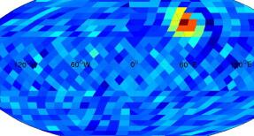
The simulated gravitational-wave backgrounds will consist of a point source and two spatially-extended distributions. The point source is not an ideal point source, but more of a Gaussian ‘blob’, since we generate it out to only $l_{\rm max}=10$ (see the first row of maps in Fig. 4).

Figure 4: Simulated maps (at a single fixed frequency) for three different anisotropic gravitational-wave backgrounds: (i) point source located at $40^{\circ}$ latitude, $60^{\circ}$ longitude having $l_{\rm max}=10$ (first row); (ii) grad-only statistically-isotropic background with $C_{l}={\rm const}$ for $2\leq l\leq 10$ (second row); (iii) curl-only statistically-isotropic background with $C_{l}={\rm const}$ for $2\leq l\leq 5$. The four columns correspond to the real and imaginary parts of $h_{+}$ and $h_{\times}$.

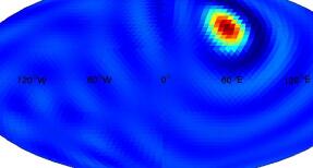
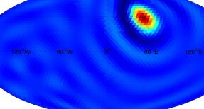
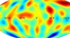
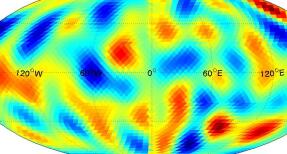
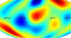
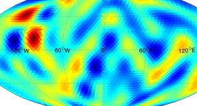
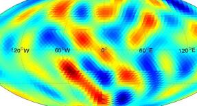
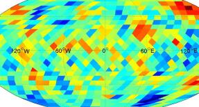
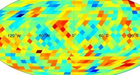
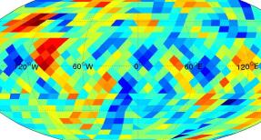
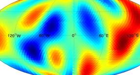
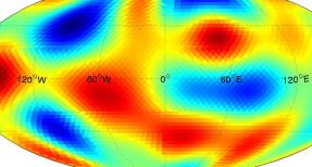
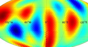
Nonetheless, it serves its purpose as being a simple yet extreme example of an anisotropic background for both $h_{+}$ and $h_{\times}$. (We also considered single-pixel point sources and found similar results, but the corresponding sky maps are not very clear.) The two spatially-extended backgrounds are a grad-only statistically isotropic background with equal contributions for multipoles $2\leq l\leq 10$, and a curl-only statistically isotropic background with equal contributions for multipoles $2\leq l\leq 5$ (see the second and third rows of Fig. 4). These last two backgrounds were also considered in Gair et al. (2014) in the context of pulsar timing arrays. It is interesting to compare the recovered sky maps for the ground-based and pulsar timing analyses, especially for the curl-only background, which cannot be recovered using timing residual data from a pulsar timing array.

Figure 5: Match as a function of number of days of observation for the 6-detector network and a noiseless point-source injection. A match value equal to 1 corresponds to perfect recovery.

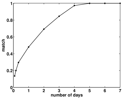
The amplitudes of the injected gravitational-wave backgrounds were chosen to give reasonable recoveries after just a few days of simulated data. For the values of the noise spectral densities $S_{I}(f)$ given in Table 1, we found that an amplitude $A=4\times 10^{-25}$ was sufficient for the three different backgrounds. (If we used a smaller value of $A$, we would have had to integrate for a longer period of time.) The faithfulness of the recovery is measured by calculating the match between the injected and maximum-likelihood-recovered sky maps,

$$\mu\equiv\frac{\frac{1}{2}({\mathbf{h}}_{\rm inj}\cdot{\mathbf{h}}_{\rm ML}+{\mathbf{h}}_{\rm ML}\cdot{\mathbf{h}}_{\rm inj})}{\sqrt{{\mathbf{h}}_{\rm inj}\cdot{\mathbf{h}}_{\rm inj}}\sqrt{{\mathbf{h}}_{\rm ML}\cdot{\mathbf{h}}_{\rm ML}}}\,.$$ (63)

This is just the coherence between the two maps. We will also construct uncertainty maps and SNR maps to evaluate how well we can recover the injections.

Figure 5 is a plot of the match as a function of the number of days of observation for the 6-detector network and a noiseless point-source injection. The match increases as the total observation time increases as expected. Note we get perfect match after 5 days of observation. This follows from the fact that the total number of data points taken by the 6-detector network over 5 days is given by $N=5~{}{\rm days}\times 60~{}{\rm samples}/{\rm day}\times 6=1800$, which is greater than the number of modes $M=2N_{\rm pix}=1536$ we are trying to recover. Thus, in the absence of noise we have (more than) enough information to completely recover the injected background after 5 days of observation. We would have complete recovery for the two other simulated backgrounds as well.

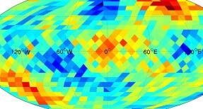
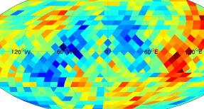
Sky maps of the recovered point-source background injected into noisy data are shown in Fig. 6. These maps are for the 6-detector network with $N=2400$ total data points, corresponding to 6.67 days of total observation. The first row shows the injected background. The second row shows the maximum-likelihood sky map estimates, which are the real and imaginary parts of the $h_{+}$, $h_{\times}$ components of ${\mathbf{h}}_{\rm ML}$. The third row shows the uncertainty maps, as specified by ${\bm{\sigma}}_{\rm ML}$, and the fourth row shows the SNR maps. The max SNR at the location of the point source is approximately 10. The match is $\mu=0.64$ for this particular simulation.

Figure 6: Recovery of the simulated point source in noise for the 6-detector network. Injected maps (first row); maximum-likehood recovered maps (second row); uncertainty map (third row); SNR map (last row). Note that the uncertainties maps for the real and imaginary parts of $h_{+}$ (or $h_{\times}$) are the same.

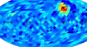
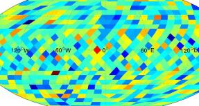
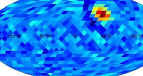
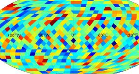
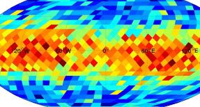
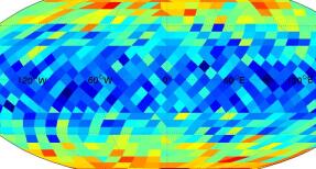
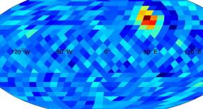
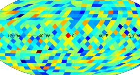
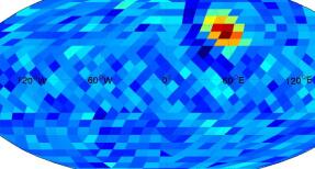
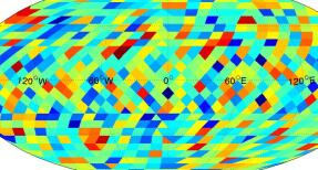
Note that the uncertainty maps for the real and imaginary parts of $h_{+}$ (or $h_{\times}$) are the same. The uncertainty values are also fairly constant over the sky, with values around $3\times 10^{-25}$. Thus, the SNR maps look very similar to the maximum-likehood maps but, of course, have different values since they represent different quantities. It is also the case that the uncertainty maps for the other simulated backgrounds (grad-only and curl-only background) will be identical to that for the point source background, since Eq. (62) for ${\bm{\sigma}}_{\rm ML}$ depends only on the response matrix ${\mathbf{R}}$ and noise covariance matrix ${\mathbf{C}}$ via (57)—i.e., it is independent of the background that one is trying to recover, at least in the weak-signal limit, which we have assumed in our analyses. So for the other two simulated backgrounds, we will show only the injected and maximum-likelihood recovered sky maps, and not the uncertainty and SNR maps.

Figure 7 is identical to Fig. 6, but for the 3-detector network having the same number of total data points ($N=2400$) as the 6-detector network. The total observation time is thus twice as long, in order to compensate for the reduction in the number of interferometers. Note that the uncertainty maps have values that are slightly larger than for the 6-detector network. Also, the match is $\mu=0.59$, which is slightly smaller than that for the 6-detector network. Thus, we see from this simulation that the 3-detector network performs nearly as well as the 6-detector network if we integrate long enough to acquire the same number of total data points. The performance of the 3-detector network is much worse than the 6-detector network if we integrate for the same observation time, since then the total number of data points for the 3-detector network is half as large (see the fourth rows of Figs. 8 and 9 below).

Figure 7: Same as Fig. 6, but for the 3-detector network having the same number of total data points ($N=2400$) as the 6-detector network. Injected maps (first row); maximum-likehood recovered maps (second row); uncertainty map (third row); SNR map (last row). The maps are more-or-less the same as for the 6-detector network shown in Fig. 6.

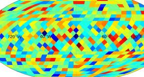
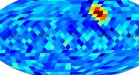
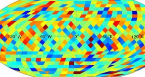
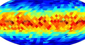
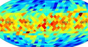
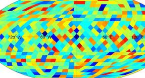
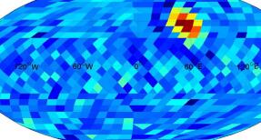
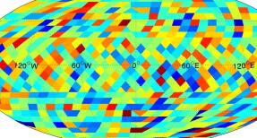
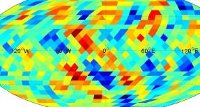
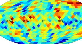
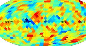
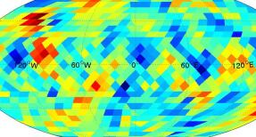
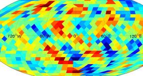
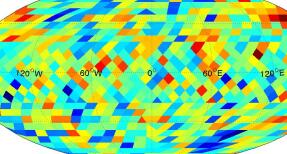
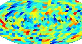
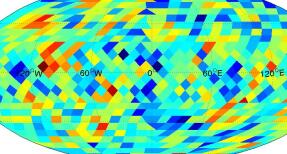
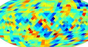
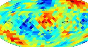
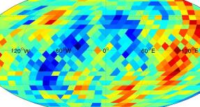
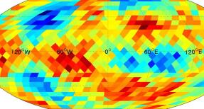
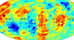
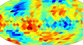
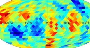
Maximum-likelihood recovered maps for the grad-only and curl-only backgrounds using the 6-detector and two 3-detector networks mentioned above (one having the same number of total data points as the 6-detector network; the other having half as many data points) are shown in Figs. 8 and 9. The corresponding match values for the grad and curl recoveries are $\mu=0.81$ and $0.85$ for the 6-detector network. For the two 3-detector networks, the match values are $\mu=0.80$ and $0.84$ when the total number of data points is the same as for the 6-detector network, and $\mu=0.55$ and $0.60$ when the total number of data points is half as many. The SNR values as a function of sky location for the different recoveries range from about $-5$ to $5$ for the strong recoveries and $-4$ to $4$ for the weaker recoveries. As can be seen from the fourth row of these two figures, when the 3-detector network has only half as many total data points as the other two networks, the structure in the grad-only and curl-only sky maps is not nearly as clearly recovered as for the other detector networks.

The most important take-home message is that the grad-only and curl-only backgrounds can both be recovered with a network of ground-based interferometers. This is in contrast to the case for a pulsar timing array, which is completely insensitive to a curl-only background (see Gair et al. (2014), and in particular Fig. 11 from that paper). As mentioned earlier, the rotational and orbital motion of the Earth synthesizes a set of virtual interferometers that sample the gravitational-wave field from many different spatial locations. This allows for the reconstruction of both grad and curl modes of the background, unlike the case for pulsar timing arrays.

Figure 8: Recovery of the grad-only background in noise. Injected maps (first row); recovered maps for the 6-detector network (second row); recovered maps for the 3-detector network having the same number of total data points ($N=2400$) as the 6-detector network (third row); recovered maps for the 3-detector network having half as many total data points ($N=1200$) as the 6-detector network (fourth row).

Figure 9: Recovery of the curl-only background in noise. Injected maps (first row); recovered maps for the 6-detector network (second row); recovered maps for the 3-detector network having the same number of total data points ($N=2400$) as the 6-detector network (third row); recovered maps for the 3-detector network having half as many total data points ($N=1200$) as the 6-detector network (fourth row).

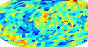
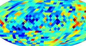
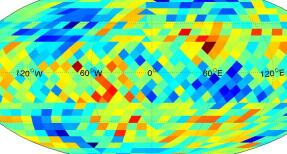
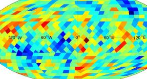
VI.6 Minimum duration between data segments for independent measurements

Having shown our map recovery techniques to be successful in the context of noisy simulated injections, we now return to an issue discussed at the end of Sec. V—namely, the minimum time increment between observations required to synthesize a network of independent virtual interferometers, and thus avoid degeneracies in the information content of our measured strain signal. We consider two cases: (i) a single AdvLIGO Livingston detector, and (ii) the full $6$-detector advanced network previously discussed. In both cases we assume a total of $1200$ strain measurements of the gravitational-wave sky have been recorded. As previously, the $h_{+}$, $h_{\times}$ components of the sky are decomposed into $768$ pixels for a total of $1536$ unknown parameters to be determined by our search. We compute maximum likelihood maps from the $1200$ observations, which are carried out over various total timespans to investigate how the match of the recovered map with the injected map scales with $\Delta t$, the time between observations.

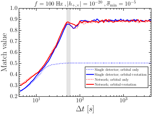
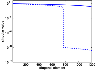
Our results are summarized in Fig. 10. For all cases, we find that the match of the recovered maps with the injected map is poor for small time increments between observations, since the detector(s) will not have moved far enough to establish independence from its previous position. With only orbital motion of a single detector, the match values are only able to plateau at $\sim\!0.5$. Adding in the influence of daily Earth rotation seems to ameliorate this poor match behaviour. The origin of this effect can be deduced from the singular values of the response matrix in both cases. This is shown in Fig. 11 for a single LIGO Livingston detector, where the addition of Earth rotation acts to break degeneracies in the response matrix and conditions it to have a much smaller dynamic range of singular values. Rotating the Earth acts to sweep the antenna beam pattern of the detector across the sky and provides additional information with which to measure the gravitational-wave background. With only orbital motion the arms of the detector remain in fixed orientations, and hence so does the detector’s antenna beam pattern. We also show in Fig. 10 the match behaviour for a full $6$-detector advanced network. In this case we already have information from multiple orientations of the antenna beam patterns by virtue of the different global placements of the detectors. Hence, the inclusion of daily Earth rotation makes little impact on the match value, which plateaus at $\sim\!0.9$ even with orbital-only motion.

The key lessons here are that Earth’s daily rotation is an important influence on top of the orbital motion of the Earth around the Sun, since it sweeps the detector antenna beam patterns across the sky to gather additional information about any gravitational-wave signal of interest. Furthermore, from Fig. 10 we can clearly see that the first peak of the match value occurs at $\sim 50-60$ s, when the detectors decorrelate from themselves for the first time (see Fig. 3) and are no longer driven in coincidence by a passing gravitational wave. With this time increment the detector’s strain measurements are effectively independent from their preceding or subsequent measurements, thereby allowing us to synthesize a large network of virtual interferometers from the daily and orbital motion of the Earth. The small dip after the first peak may be due to the detectors being driven in anti-coincidence, thereby losing some of their independence. However, the match value recovers in the limit of large $\Delta t$, since the detectors are then separated by several gravitational-wave wavelengths and this behaviour is averaged out.

Figure 10: Match values for various noisy map injections (averaged over $500$ noise realizations) as a function of the time increment between $1200$ observations, for a single detector and a $6$-detector network. For a single detector, orbital-only motion is only able to achieve a match value of $\sim 0.5$ at large $\Delta t$. Daily rotation provides additional information by sweeping the antenna beam pattern across the sky, thus giving excellent plateau match values of $\sim 0.9$. The global placement of a network of detectors (and their differing antenna beam pattern orientations) gives excellent match values even for orbital-only motion, and daily rotation does not significantly improve this match. We see that the first peak in the match value occurs at $\sim 50-60$ seconds (shown as a grey strip), when the detectors first decorrelate from themselves and are no longer driven in coincidence by a passing gravitational wave. The small dip after the first peak is due to the virtual detectors being driven in anti-coincidence by the gravitational wave, thereby losing some of their independence and diminishing the match. However at larger $\Delta t$ this behavior is averaged out over several gravitational-wave wavelengths, allowing the match value to recover.

Figure 11: Singular values of the response matrix for a single LIGO-Livingston interferometer, for $1200$ total observations with $\Delta t=(1~{}{\rm sidereal\ day})/60\approx 1436~{}{\rm s}$. (The singular values are normalized by the largest singular value, corresponding to the first diagonal element.) The dashed blue line shows the singular values when the detector is affixed to an Earth undergoing orbital motion only, whilst the solid blue line shows the singular values when the Earth is both rotating and orbiting. This indicates that in the orbiting-only case, regularization of the response matrix at machine-level precision ($\epsilon\sim 10^{-16}$) will not remove the very small singular values after diagonal element 768, requiring a more stringent cutoff level. In contrast, when the extra influence of the Earth’s rotation is introduced, the additional information provided by the changing detector arm orientations (which sweep the antenna beam pattern across the sky) acts to drastically improve the conditioning of the response matrix.

VII Discussion

We have presented a new method for mapping the gravitational-wave sky using a network of ground-based laser interferometers. This method extends the formalisms developed in Gair et al. (2014); Cornish and van Haasteren (2014), which were originally applied to the case of pulsar timing arrays. We have shown that we can recover both the gradient and curl components of a gravitational-wave background, as a consequence of the spatial separation of the individual interferometers in the network, or of a single interferometer at different times during its rotational and orbital motion around the Sun. This is in contrast to the case for a pulsar timing array, which is completely insensitive to the curl modes. Also, by mapping both the amplitude and phase of $h_{+}(f,\hat{k})$ and $h_{\times}(f,\hat{k})$ as functions of direction on the sky (as referenced from the SSB), our method extends previous approaches Allen and Ottewill (1997); Cornish (2001); Mitra et al. (2008); Thrane et al. (2009); Abadie et al. (2011); Mingarelli et al. (2013); Taylor and Gair (2013) for anisotropic backgrounds, which map the distribution of gravitational-wave power, $|h_{+}|^{2}+|h_{\times}|^{2}$. Our formalism can be cast in terms of either the traditional $+$ and $\times$ polarization modes of the background $\{h_{+}(f,\hat{k}),h_{\times}(f,\hat{k})\}$, or the gradient and curl modes $\{a^{G}_{(lm)}(f),a^{C}_{(lm)}(f)\}$, with respect to a decomposition of the metric perturbations in terms of spin-weighted or tensor (gradient and curl) spherical harmonics Gair et al. (2014).

The results of the simulations presented in Sec. VI.5 can be thought as a proof-of-principle demonstration of the general map-making formalism described in the rest of the paper. The actual analysis of real data from a network of advanced interferometers will most likely differ from this simplified scenario in several ways:

(i) The amplitudes of the simulated backgrounds were chosen to be sufficently large, so as to allow for fairly decent recovery after only a few days of observation. Much weaker backgrounds will require an increased observation time, of order months or years, noting that the (power) signal-to-noise ratio scales like $A^{2}\sqrt{T}$, where $A$ is the amplitude of the background and $T$ is the total observation time.

(ii) For initial analyses, it might be easier to work in the tensor spherical harmonic basis, and estimate the grad and curl components of the background $\{a^{G}_{(lm)}(f)$, $a^{C}_{(lm)}(f)\}$ out to some relatively small value of $l_{\rm max}$, e.g., $l_{\rm max}=10$. This would reduce the number of modes that we would need to recover from $2N_{\rm pix}$ ($=1536$ for example) to $2N_{\rm modes}=234$ at each discrete frequency. The estimates of the grad and curl components can then be converted to sky maps of $h_{+}(f,\hat{k})$, $h_{\times}(f,\hat{k})$ using (12).

(iii) Varying noise levels in the detectors (on a time scale $\gtrsim$ the segment duration $\tau$ of our short-term Fourier transforms) will complicate somewhat the expression for the noise covaraince matrix ${\mathbf{C}}$. The $N_{d}$ block matrices that enter the expression for ${\mathbf{C}}$ will no longer be proportional to the unit matrix $\mathds{1}_{N_{t}\times N_{t}}$, but rather will have diagonal elements proportional to $S_{I}(f;t_{Ii})$, $i=1,2,\cdots,N_{t}$, reflecting the time-varying noise levels in detector $I$.

(iv) As ground-based interferometers are broad-band detectors, we will have measurements at a set of discrete frequencies $f_{j}$, $j=1,2,\cdots,N_{f}$, where $N_{f}\sim$ several hundred to a few thousand depending on the frequency bin size $\delta f$. For initial analyses, it will probably be simplest to average the estimates of $h_{+}(f_{j},\hat{k})$, $h_{\times}(f_{j},\hat{k})$ over the different frequency components.

(v) If one would like to compare the consistency of different models of a stochastic background with the measured data—e.g., is the measured data consistent with an unpolarized, isotropic background or with a background having a non-zero dipole component or with correlated emission on the sky, etc.—a Bayesian formulation of the problem would be more appropriate. The different models would be defined by the appropriate choice of variables for the stochastic background and prior probably distributions for these variables. Bayesian model selection would then be used to select between the competing models.

Perhaps the most compelling reason for using the formalism presented here is that it provides a completely generic approach to mapping the gravitational-wave sky. It allows us to construct a map of the background that extracts all of the information that is possible to extract from the measured data. With the advanced ground-based interferometers coming on-line at the end of this year, and with the first detection of gravitational waves expected to follow shortly thereafter, it seems appropriate to utilize approaches such as this that attempt to maximize the science return of the data.

Appendix A Derivation of gradient and curl response functions

Here we derive the gradient and curl response functions for an interferometer in the small-antenna limit, allowing for a non-zero displacement $\vec{x}_{0}$ of the vertex of the interferometer from the origin of coordinates.

Expressions for the response functions evaluated in a reference frame whose origin is located at the vertex of the interferometer were derived in Appendix D of Gair et al. (2014):

$$\bar{R}^{G}_{(lm)}(f) =\delta_{l2}\,\frac{4\pi}{5}\sqrt{\frac{1}{3}}\left[Y_{2m}(\hat{u})-Y_{2m}(\hat{v})\right]\,,$$ (64)

$$\bar{R}^{C}_{(lm)}(f) =0\,,$$

where $\hat{u}$, $\hat{v}$ are unit vectors in the directions of the two arms of the interferometer. We have put bars on the above expressions to distinguish them from similar unbarred quantities that we will calculate in a reference frame whose origin is at the solar system barycentre (SSB). Note that $\bar{R}^{G}_{(lm)}$ is independent of frequency and is non-zero only for the quadrupole modes, $l=2$.

Under a translation of reference frames from the SSB to the vertex of the interferometer located at $\vec{x}_{0}$, the Fourier components $h_{ab}(f,\hat{k})$ of the metric perturbations $h_{ab}(t,\vec{x})$ in the “cosmic” (or SSB) frame transform to

$$\bar{h}_{ab}(f,\hat{k})=h_{ab}(f,\hat{k})e^{-i2\pi f\hat{k}\cdot\vec{x}_{0}/c}$$ (65)

in the detector frame. The correponding mode expansions in the two frames are given by

$$h_{ab}(f,\hat{k}) =\sum_{(lm)}\sum_{P}a^{P}_{(lm)}(f)Y_{(lm)ab}^{P}(\hat{k})\,,$$ (66)

$$\bar{h}_{ab}(f,\hat{k}) =\sum_{(lm)}\sum_{P}\bar{a}^{P}_{(lm)}(f)Y_{(lm)ab}^{P}(\hat{k})\,.$$

This last equation for $\bar{h}_{ab}(f,\hat{k})$ can be inverted to find $\bar{a}^{P}_{(lm)}(f)$ in terms of $a^{P}_{(lm)}(f)$ using (65) and the orthogonality of the gradient and curl spherical harmonics:

$$\bar{a}^{P}_{(lm)}(f) =\int_{S^{2}}{\rm d}^{2}\Omega_{\hat{k}}\>\bar{h}_{ab}(f,\hat{k})Y^{P}_{(lm)}{}^{ab\,*}(\hat{k})$$ (67)

$$=\int_{S^{2}}{\rm d}^{2}\Omega_{\hat{k}}\>h_{ab}(f,\hat{k})e^{-i2\pi f\hat{k}\cdot\vec{x}_{0}/c}\,Y^{P}_{(lm)}{}^{ab\,*}(\hat{k})$$

$$=\int_{S^{2}}{\rm d}^{2}\Omega_{\hat{k}}\ \sum_{(l^{\prime}m^{\prime})}\sum_{P^{\prime}}a^{P^{\prime}}_{(l^{\prime}m^{\prime})}(f)Y^{P^{\prime}}_{(l^{\prime}m^{\prime})ab}(\hat{k})e^{-i2\pi f\hat{k}\cdot\vec{x}_{0}/c}\,Y^{P}_{(lm)}{}^{ab\,*}(\hat{k})\,.$$

Using the identity:

$$e^{-i2\pi f\hat{k}\cdot\vec{x}_{0}/c}=4\pi\sum_{L=0}^{\infty}(-i)^{L}j_{L}(\alpha)\sum_{M=-L}^{L}Y^{*}_{LM}(\hat{x}_{0})Y_{LM}(\hat{k})\,,\qquad\alpha\equiv 2\pi f|\vec{x}_{0}|/c\,,$$ (68)

we obtain

$$\bar{a}^{P}_{(lm)}(f)=\sum_{(l^{\prime}m^{\prime})}\sum_{P^{\prime}}a^{P^{\prime}}_{(l^{\prime}m^{\prime})}(f)\sum_{L=0}^{\infty}\sum_{M=-L}^{L}4\pi(-i)^{L}j_{L}(\alpha)Y^{*}_{LM}(\hat{x}_{0})\int_{S^{2}}{\rm d}^{2}\Omega_{\hat{k}}\ Y^{P^{\prime}}_{(l^{\prime}m^{\prime})ab}(\hat{k})Y^{P}_{(lm)}{}^{ab\,*}(\hat{k})Y_{LM}(\hat{k})$$ (69)

relating the mode coefficients in the two frames.

To make the connection between the mode coefficients and the corresponding response functions, we note that the detector response $\tilde{r}(f)$ (or $r(t)$) to the gravitational-wave background will have the same value regardless of which frame we choose to evaluate it in. Thus,

$$\tilde{r}(f) =\sum_{(lm)}\sum_{P}\bar{R}^{P}_{(lm)}\bar{a}^{P}_{(lm)}(f)$$ (70)

$$=\sum_{m=-2}^{2}\bar{R}^{G}_{(2m)}\bar{a}^{G}_{(2m)}(f)$$

$$=\sum_{m=-2}^{2}\bar{R}^{G}_{(2m)}\sum_{(l^{\prime}m^{\prime})}\sum_{P^{\prime}}a^{P^{\prime}}_{(l^{\prime}m^{\prime})}(f)\sum_{L=0}^{\infty}\sum_{M=-L}^{L}4\pi(-i)^{L}j_{L}(\alpha)Y^{*}_{LM}(\hat{x}_{0})\int_{S^{2}}{\rm d}^{2}\Omega_{\hat{k}}\ Y^{P^{\prime}}_{(l^{\prime}m^{\prime})ab}(\hat{k})Y^{G}_{(2m)}{}^{ab\,*}(\hat{k})Y_{LM}(\hat{k})$$

$$=\sum_{(l^{\prime}m^{\prime})}\sum_{P^{\prime}}R^{P^{\prime}}_{(l^{\prime}m^{\prime})}(f)a^{P^{\prime}}_{(l^{\prime}m^{\prime})}(f)\,,$$

where

$$R^{P}_{(lm)}(f)=\sum_{m^{\prime}=-2}^{2}\sum_{L=0}^{\infty}\sum_{M=-L}^{L}\bar{R}^{G}_{(2m^{\prime})}4\pi(-i)^{L}j_{L}(\alpha)Y^{*}_{LM}(\hat{x}_{0})\int_{S^{2}}{\rm d}^{2}\Omega_{\hat{k}}\ Y^{P}_{(lm)ab}(\hat{k})Y^{G}_{(2m^{\prime})}{}^{ab\,*}(\hat{k})Y_{LM}(\hat{k})\,.$$ (71)

We can write this last expression explicitly in terms of Wigner-3$j$ symbols if we replace the grad and curl spherical harmonics in the integral by spin-2 spherical harmonics using:

$$Y^{G}_{(lm)ab}(\hat{k})Y^{G}_{(2m^{\prime})}{}^{ab\,*}(\hat{k}) =\frac{1}{2}\left[{}_{-2}Y_{lm}(\hat{k}){}_{-2}Y_{2m^{\prime}}^{*}(\hat{k})+{}_{2}Y_{lm}(\hat{k}){}_{2}Y_{2m^{\prime}}^{*}(\hat{k})\right]\,,$$ (72)

$$Y^{C}_{(lm)ab}(\hat{k})Y^{G}_{(2m^{\prime})}{}^{ab\,*}(\hat{k}) =\frac{1}{2i}\left[{}_{-2}Y_{lm}(\hat{k}){}_{-2}Y_{2m^{\prime}}^{*}(\hat{k})-{}_{2}Y_{lm}(\hat{k}){}_{2}Y_{2m^{\prime}}^{*}(\hat{k})\right]\,.$$

This leads to

$$R^{G}_{(lm)}(f)= \sum_{m^{\prime}=-2}^{2}\sum_{L=0}^{\infty}\sum_{M=-L}^{L}\bar{R}^{G}_{(2m^{\prime})}4\pi(-i)^{L}j_{L}(\alpha)Y^{*}_{LM}(\hat{x}_{0})$$ (73)

$$\frac{(-1)^{m^{\prime}}}{2}\sqrt{\frac{(2\cdot 2+1)(2l+1)(2L+1)}{4\pi}}\left(\begin{array}[]{ccc}2&l&L\\ -m^{\prime}&m&M\end{array}\right)\left[\left(\begin{array}[]{ccc}2&l&L\\ -2&2&0\end{array}\right)+\left(\begin{array}[]{ccc}2&l&L\\ 2&-2&0\end{array}\right)\right]\,,$$

$$R^{C}_{(lm)}(f)= \sum_{m^{\prime}=-2}^{2}\sum_{L=0}^{\infty}\sum_{M=-L}^{L}\bar{R}^{G}_{(2m^{\prime})}4\pi(-i)^{L}j_{L}(\alpha)Y^{*}_{LM}(\hat{x}_{0})$$

$$\frac{(-1)^{m^{\prime}}}{2i}\sqrt{\frac{(2\cdot 2+1)(2l+1)(2L+1)}{4\pi}}\left(\begin{array}[]{ccc}2&l&L\\ -m^{\prime}&m&M\end{array}\right)\left[\left(\begin{array}[]{ccc}2&l&L\\ -2&2&0\end{array}\right)-\left(\begin{array}[]{ccc}2&l&L\\ 2&-2&0\end{array}\right)\right]\,.$$

These expressions can be further simplified using the symmetry property

$$\left(\begin{array}[]{ccc}l_{1}&l_{2}&l\\ m_{1}&m_{2}&m\end{array}\right)=(-1)^{l_{1}+l_{2}+l}\left(\begin{array}[]{ccc}l_{1}&l_{2}&l\\ -m_{1}&-m_{2}&-m\end{array}\right)$$ (74)

to eliminate one the Wigner 3-$j$ symbols in terms of the other, and the triangle inequality

$$|l_{1}-l_{2}|\leq l\leq l_{1}+l_{2}\quad\Rightarrow\quad l-2\leq L\leq l+2$$ (75)

to collapse the infinite sums over $L$ to sums over just 5 terms. The final expressions are

$$R^{G}_{(lm)}(f)= \sum_{m^{\prime}=-2}^{2}\sum_{L=l-2}^{l+2}\sum_{M=-L}^{L}\bar{R}^{G}_{(2m^{\prime})}4\pi(-i)^{L}j_{L}(\alpha)Y^{*}_{LM}(\hat{x}_{0})$$ (76)

$$\frac{(-1)^{m^{\prime}}}{2}\sqrt{\frac{(2\cdot 2+1)(2l+1)(2L+1)}{4\pi}}\left(\begin{array}[]{ccc}2&l&L\\ -m^{\prime}&m&M\end{array}\right)\left(\begin{array}[]{ccc}2&l&L\\ 2&-2&0\end{array}\right)\left[(-1)^{l+L}+1\right]\,,$$

$$R^{C}_{(lm)}(f)= \sum_{m^{\prime}=-2}^{2}\sum_{L=l-2}^{l+2}\sum_{M=-L}^{L}\bar{R}^{G}_{(2m^{\prime})}4\pi(-i)^{L}j_{L}(\alpha)Y^{*}_{LM}(\hat{x}_{0})$$

$$\frac{(-1)^{m^{\prime}}}{2i}\sqrt{\frac{(2\cdot 2+1)(2l+1)(2L+1)}{4\pi}}\left(\begin{array}[]{ccc}2&l&L\\ -m^{\prime}&m&M\end{array}\right)\left(\begin{array}[]{ccc}2&l&L\\ 2&-2&0\end{array}\right)\left[(-1)^{l+L}-1\right]\,.$$

The Wigner 3-$j$ symbol selection rule

$$-m^{\prime}+m+M=0$$ (77)

implies that the sum over $M$ collapses to only those values satisfying $M=m^{\prime}-m$ and $|M|<L$. Note also that in a reference frame with the $z$-axis chosen along $\hat{x}_{0}$,

$$Y^{*}_{LM}(\hat{x}_{0})=Y^{*}_{LM}(0,\phi)=\delta_{M0}\,\sqrt{\frac{2L+1}{4\pi}}\,,$$ (78)

so for this case the sum over $M$ reduces to just the $M=0$ value. The selection rule $-m^{\prime}+m=0$ and $|m^{\prime}|\leq 2$ then imply non-zero values for only $|m|\leq 2$ in this special frame.

Appendix B Equivalence of whitened and non-whitened analyses

As discussed in Sec. VI.2, we are interested in finding the maximum-likelihood value ${\mathbf{h}}_{\rm ML}$ of the likelihood function

$$p({\mathbf{d}}|{\mathbf{C}},{\mathbf{h}})\propto\exp\left[-({\mathbf{d}}-{\mathbf{R}}{\mathbf{h}})^{\dagger}{\mathbf{C}}^{-1}({\mathbf{d}}-{\mathbf{R}}{\mathbf{h}})\right]\,,$$ (79)

when the Fisher matrix ${\mathbf{F}}\equiv{\mathbf{R}}^{\dagger}{\mathbf{C}}^{-1}{\mathbf{R}}$ is not invertible. One approach, described in Gair et al. (2014), is to work with the SVD of the response matrix ${\mathbf{R}}$:

$${\mathbf{R}}={\mathbf{U}}{\bm{\Sigma}}{\mathbf{V}}^{\dagger}\,.$$ (80)

In general we can write ${\mathbf{U}}=[{\mathbf{U}}_{r}{\mathbf{U}}_{n}]$, where ${\mathbf{U}}_{r}$ is an $N\times r$ matrix denoting the range of the response matrix ${\mathbf{R}}$, where $r$ equals the number of non-zero singular values in ${\bm{\Sigma}}$. We then replace ${\mathbf{R}}{\mathbf{h}}$ in the likelihood by ${\mathbf{U}}_{r}{\mathbf{b}}$, where ${\mathbf{b}}$ is a vector of dimension $r$, and then proceed as for a non-singular response. The maximum-likelihood value for ${\mathbf{b}}$ is then

$${\mathbf{b}}_{\rm ML}=({\mathbf{U}}_{r}^{\dagger}{\mathbf{C}}^{-1}{\mathbf{U}}_{r})^{-1}{\mathbf{U}}_{r}^{\dagger}{\mathbf{C}}^{-1}{\mathbf{d}}\,,$$ (81)

and the corresponding maximum-likelihood estimate of the gravitational-wave sky is

$${\mathbf{h}}_{\rm ML}={\mathbf{V}}{\bm{\Sigma}}_{r}^{+}{\mathbf{b}}_{\rm ML}\,,$$ (82)

where ${\bm{\Sigma}}_{r}$ is the $r\times M$ dimensional matrix obtained by crossing out the last $N-r$ rows of ${\bm{\Sigma}}$, and ${\bm{\Sigma}}_{r}^{+}$ is the pseudo-inverse of ${\bm{\Sigma}}_{r}$, obtained by taking the reciprocal of each non-zero singular value of ${\bm{\Sigma}}_{r}$, and then transposing the resulting matrix.

An alternative approach, which we described in Sec. VI.2, is to work with the the whitened data $\bar{\mathbf{d}}\equiv{\mathbf{L}}^{\dagger}{\mathbf{d}}$ and whitened response matrix $\bar{\mathbf{R}}\equiv{\mathbf{L}}^{\dagger}{\mathbf{R}}$, where ${\mathbf{L}}$ is a lower triangular matrix defined by the Cholesky decomposition of the inverse covariance matrix, ${\mathbf{C}}^{-1}={\mathbf{L}}{\mathbf{L}}^{\dagger}$. Working with the SVD of $\bar{\mathbf{R}}$:

$$\bar{\mathbf{R}}=\bar{\mathbf{U}}\bar{\bm{\Sigma}}\bar{\mathbf{V}}^{\dagger}\,,$$ (83)

we have

$${\mathbf{h}}_{\rm ML}=\bar{\mathbf{V}}\bar{\bm{\Sigma}}^{+}\bar{\mathbf{U}}^{\dagger}\bar{\mathbf{d}}\,.$$ (84)

Now the SVD of a product cannot be simply written in terms of the SVDs of the individual matrices. However, we can show the equivalence of these two approaches for maximizing the likelihood, by working with the equivalent likelihood that was introduced in the first approach, i.e.,

$$p({\mathbf{d}}|{\mathbf{C}},{\mathbf{h}})\propto\exp\left[-({\mathbf{d}}-{\mathbf{U}}_{r}{\mathbf{b}})^{\dagger}{\mathbf{C}}^{-1}({\mathbf{d}}-{\mathbf{U}}_{r}{\mathbf{b}})\right]\,,$$ (85)

and obtaining ${\mathbf{h}}_{\rm ML}$ from ${\mathbf{b}}_{\rm ML}$ using Eq. (82). The first approach requires no modification, but for the second approach we now need the SVD of the whitened ${\mathbf{U}}_{r}$ matrix, ${\mathbf{L}}^{\dagger}{\mathbf{U}}_{r}$:

$${\mathbf{L}}^{\dagger}{\mathbf{U}}_{r}=\tilde{\mathbf{U}}\tilde{\bm{\Sigma}}\tilde{\mathbf{V}}^{\dagger}\,,$$ (86)

for which

$${\mathbf{b}}_{\rm ML}=\tilde{\mathbf{V}}\tilde{\bm{\Sigma}}^{+}\tilde{\mathbf{U}}^{\dagger}\bar{\mathbf{d}}\,.$$ (87)

Since we are now working only with the range of ${\mathbf{R}}$ and the noise covariance matrix ${\mathbf{C}}$ is positive definite, the rank of ${\mathbf{L}}^{\dagger}{\mathbf{U}}_{r}$ must equal the rank of ${\mathbf{U}}_{r}$. As before, we can write $\tilde{\mathbf{U}}=[\tilde{\mathbf{U}}_{r}\tilde{\mathbf{U}}_{n}]$, where $\tilde{\mathbf{U}}_{r}$ is an $N\times r$ matrix, which gives the range of ${\mathbf{L}}^{\dagger}{\mathbf{U}}_{r}$. Thus, we can equivalently write Eq. (86) as

$${\mathbf{L}}^{\dagger}{\mathbf{U}}_{r}=\tilde{\mathbf{U}}_{r}\tilde{\bm{\Sigma}}_{r}\tilde{\mathbf{V}}^{\dagger}\,,$$ (88)

where $\tilde{\bm{\Sigma}}_{r}$ is an invertible, square $r\times r$ matrix obtained, as before, by crossing out the last $N-r$ rows of $\tilde{\bm{\Sigma}}$. From this last equation we now see that

$$\tilde{\mathbf{U}}_{r}={\mathbf{L}}^{\dagger}{\mathbf{U}}_{r}\tilde{\mathbf{V}}\tilde{\bm{\Sigma}}_{r}^{-1}\,,$$ (89)

and

$${\mathbf{b}}_{\rm ML} =\tilde{\mathbf{V}}\tilde{\bm{\Sigma}}_{r}^{-1}\tilde{\mathbf{U}}_{r}^{\dagger}\bar{\mathbf{d}}$$ (90)

$$=\tilde{\mathbf{V}}\tilde{\bm{\Sigma}}_{r}^{-1}\tilde{\bm{\Sigma}}_{r}^{-1}\tilde{\mathbf{V}}^{\dagger}{\mathbf{U}}_{r}^{\dagger}{\mathbf{L}}\bar{\mathbf{d}}$$

$$=({\mathbf{U}}_{r}^{\dagger}{\mathbf{C}}^{-1}{\mathbf{U}}_{r})^{-1}{\mathbf{U}}_{r}^{\dagger}{\mathbf{C}}^{-1}{\mathbf{d}}\,,$$

where the final equality follows from the observation that ${\mathbf{U}}_{r}^{\dagger}{\mathbf{C}}^{-1}{\mathbf{U}}_{r}={\mathbf{U}}_{r}^{\dagger}{\mathbf{L}}{\mathbf{L}}^{\dagger}{\mathbf{U}}_{r}=\tilde{\mathbf{V}}\tilde{\bm{\Sigma}}_{r}^{2}\tilde{\mathbf{V}}^{\dagger}$ (which is a consequence of Eq. (88)). We have thus recovered the result given in Eq. (81), which was obtained without whitening the data.

References

- Gair et al. (2014) J. Gair, J. D. Romano, S. Taylor, and C. M. F. Mingarelli, Phys. Rev. D 90, 082001 (2014), eprint 1406.4664.
- Cornish and van Haasteren (2014) N. J. Cornish and R. van Haasteren (2014), eprint arXiv:1406.4511.
- Allen and Ottewill (1997) B. Allen and A. Ottewill, Physical Review D 56, 545 (1997).
- Cornish (2001) N. J. Cornish, Classical and Quantum Gravity 18, 4277 (2001).
- Mitra et al. (2008) S. Mitra, S. Dhurandhar, T. Souradeep, A. Lazzarini, V. Mandic, S. Bose, and S. Ballmer, Physical Review D 77, 1550 (2008).
- Thrane et al. (2009) E. Thrane, S. Ballmer, J. D. Romano, D. T. Sanjit Mitra, S. Bose, and V. Mandic, Physical Review D 80, 122002 (2009).
- Abadie et al. (2011) J. Abadie et al., Phys. Rev. Lett. 107, 271102 (2011), URL http://link.aps.org/doi/10.1103/PhysRevLett.107.271102.
- Mingarelli et al. (2013) C. M. F. Mingarelli, T. Sidery, I. Mandel, and A. Vecchio, Physical Review D 88, 062005 (2013).
- Taylor and Gair (2013) S. R. Taylor and J. R. Gair, Physical Review D 88, 084001 (2013).
- The LIGO Scientific Collaboration et al. (2015) The LIGO Scientific Collaboration, J. Aasi, B. P. Abbott, R. Abbott, T. Abbott, M. R. Abernathy, K. Ackley, C. Adams, T. Adams, P. Addesso, et al., Classical and Quantum Gravity 32, 074001 (2015), eprint 1411.4547.
- Acernese et al. (2015) F. Acernese et al. (VIRGO), Class.Quant.Grav. 32, 024001 (2015), eprint 1408.3978.
- Danzmann and LISA Study (1996) K. Danzmann and LISA Study, Classical and Quantum Gravity 13, 247 (1996).
- Amaro-Seoane et al. (2012) P. Amaro-Seoane, S. Aoudia, S. Babak, P. Binetruy, E. Berti, A. Bohe, C. Caprini, M. Colpi, et al., Classical and Quantum Gravity 29, 124016 (2012), eprint arXiv:1202.0839 [gr-qc].
- Amaro-Seoane et al. (2013) P. Amaro-Seoane, S. Aoudia, S. Babak, P. Binétruy, E. Berti, A. Bohé, C. Caprini, M. Colpi, N. J. Cornish, K. Danzmann, et al., GW Notes, Vol. 6, p. 4-110 6, 4 (2013), eprint 1201.3621.
- Phinney et al. (2004) S. Phinney et al., NASA Mission Concept Study (2004).
- Kamionkowski et al. (1997) M. Kamionkowski, A. Kosowsky, and A. Stebbins, Physical Review D 55, 7368 (1997).
- Foster and Backer (1990) R. S. Foster and D. C. Backer, Astrophysical Journal 361, 300 (1990).
- Newman and Penrose (1966) E. T. Newman and R. Penrose, Journal of Mathematical Physics 7, 863 (1966).
- Goldberg et al. (1967) J. N. Goldberg et al., Journal of Mathematical Physics 8, 2115 (1967).
- Mingarelli and Sidery (2014) C. M. F. Mingarelli and T. Sidery, Phys. Rev. D 90, 062011 (2014), eprint 1408.6840.
- Wigner (1959) E. P. Wigner, Group Theory and Its Application to the Quantum Mechanics of Atomic Spectra, expanded and improved ed. (Academic Press, New York, 1959).
- Messiah (1962) A. Messiah, Quantum Mechanics, Vol. 2 (North Holland, Amsterdam, Netherlands, 1962).
- Flanagan (1993) É. É. Flanagan, Physical Review D 48, 2389 (1993).
- Allen and Romano (1999) B. Allen and J. Romano, Physical Review D 59, 102001 (1999).
- Ain et al. (2015) A. Ain, P. Dalvi, and S. Mitra (2015), eprint arxiv:1504.01714 [gr-qc].
- Abbott et al. (2004) B. Abbott et al., Physical Review D 69, 122004 (2004), eprint gr-qc/0312088.
- Press et al. (1992) W. H. Press, S. A. Teukolsky, W. T. Vetterling, and B. P. Flannery, Numerical Recipes in C (Cambridge University Press, 1992).
- Schutz (2011) B. F. Schutz, Classical and Quantum Gravity 28, 125023 (2011), eprint 1102.5421.
- (29) Advanced LIGO anticipated sensitivity curves, https://dcc.ligo.org/LIGO-T0900288/public, accessed: 2015-04-26.
- (30) Advanced Virgo, https://wwwcascina.virgo.infn.it/advirgo/, accessed: 2015-04-26.
- (31) KAGRA Sensitivity Curve; KAGRA-VRSE(D), http://gwcenter.icrr.u-tokyo.ac.jp/en/researcher/parameter, accessed: 2015-04-26.
- Górski et al. (2005) K. M. Górski, E. Hivon, A. J. Banday, B. D. Wandelt, F. K. Hansen, M. Reinecke, and M. Bartelmann, Astrophysical Journal 622, 759 (2005).