An NPZ Model with State-Dependent Delay due to Size-Structure in Juvenile Zooplankton

Matt Kloosterman111mklooste@uwaterloo.ca    Sue Ann Campbell    Francis J. Poulin
Department of Applied Mathematics,
University of Waterloo, Waterloo, ON, Canada N2L 3G1
Abstract

The study of planktonic ecosystems is important as they make up the bottom trophic levels of aquatic food webs. We study a closed Nutrient-Phytoplankton-Zooplankton (NPZ) model that includes size structure in the juvenile zooplankton. The closed nature of the system allows the formulation of a conservation law of biomass that governs the system. The model consists of a system of nonlinear ordinary differential equation coupled to a partial differential equation. We are able to transform this system into a system of delay differential equations where the delay is of threshold type and is state-dependent. The system of delay differential equations can be further transformed into one with fixed delay. Using the different forms of the model we perform a qualitative analysis of the solutions, which includes studying existence and uniqueness, positivity and boundedness, local and global stability, and conditions for extinction. Key parameters that are explored are the total biomass in the system and the maturity level at which the juvenile zooplankton reach maturity. Numerical simulations are also performed to verify our analytical results.

1 Introduction

Nutrient-Phytoplankton-Zooplankton (NPZ) models are used to describe the bottom two trophic levels of an aquatic ecosystem. As is the case with many ecological models, they range from very simple to very complex. Simple models, such as the Lotka-Volterra system [16], are beneficial in that one can obtain analytical results more easily, but often suffer from lack of realism. On the other hand, complex models may theoretically represent a more accurate description of reality, but may be difficult or impossible to understand in any general way, and may be useless without precise and accurate parameter values. A lot of structure can be given to an NPZ model, such as size-dependence and spatial dependence, and this structure leads to rich modelling possibilities such as size-dependent parameters and coupling with external factors like fluid dynamics or higher predation. To strike a balance, it may be useful to start with a simple model that focuses on one factor affecting the ecosystem, and use it to obtain analytical results and study general trends. For an introduction in the construction of NPZ models, see [6].

We will focus on the role of maturity in the juvenile zooplankton population within an ecosystem while keeping all other factors as simple as possible. In this vain, a simple NPZ model is coupled with a standard linear first-order PDE that describes the spectrum of the juvenile zooplankton population as a function of time and maturity. It is a known result that this type of PDE is closely related to delay equations. Examples of population models where time delay is a consequence of age structure can be found in [10], [1], [23], [2]. We will be considering size structure where the rate of growth of the juvenile zooplankton is permitted to depend on the concentration of the phytoplankton. With this assumption, the delay in the related delay equation is not explicitly defined, but rather defined implicitly through a threshold-type condition. Consequently, systems with this type of delay are known as threshold delay differential equations. They have been studied in the case of a single population in [20] and for an insect species in [17], for example. These models operate under the assumption that maturation occurs when an immature individual accumulates enough of some quantity, such as size or weight. Other applications include red blood cell production [15] and immunology [25].

Our model is formulated in such a way that biomass is conserved. In other words, we are considering a closed ecosystem with no mass being added to or subtracted from the system. NPZ models with this property have been studied, for example, by [7] and [26]. A typical property of these systems is that the amount of biomass, which is determined by initial conditions, plays a crucial role in determining the types of dynamics that can and do occur. Most notably, an insufficient amount of biomass leads to the extinction of plankton; either the zooplankton only, or both the phytoplankton and zooplankton.

2 Structured Model

We consider a Nutrient-Phytoplankton-Zooplankton (NPZ) model in which the zooplankton population is split into a mature class and a juvenile class. We will consider the juvenile class as a function of time and maturity, denoted ρ(t,s)𝜌𝑡𝑠\rho(t,s). Maturity is considered to be an abstract quantity, of which the juvenile zooplankton much accumulate enough in order to enter adulthood. The total concentration of immature zooplankton with maturity levels between s1subscript𝑠1s_{1} and s2subscript𝑠2s_{2} at time t𝑡t is then s1s2ρ(t,s)𝑑ssuperscriptsubscriptsubscript𝑠1subscript𝑠2𝜌𝑡𝑠differential-d𝑠\int_{s_{1}}^{s_{2}}\rho(t,s)\,ds. We restrict s𝑠s to the interval [0,m]0𝑚[0,m], where m𝑚m is the required level of maturity for adulthood. The nutrient, phytoplankton, and mature zooplankton variables will therefore only depend on time.

Since the zooplankton feed on phytoplankton, we will assume that the growth rate of the juvenile zooplankton depends on the quantity of phytoplankton present in the system. We will denote this dependence as R(P(t))𝑅𝑃𝑡R(P(t)).

The following equations model the ecosystem and we will refer to it as the PDE1 model.

dN(t)dt=μP(t)f(N(t))+λP(t)+δZ(t)+(1γ)gZ(t)h(P(t))𝑑𝑁𝑡𝑑𝑡𝜇𝑃𝑡𝑓𝑁𝑡𝜆𝑃𝑡𝛿𝑍𝑡1𝛾𝑔𝑍𝑡𝑃𝑡\displaystyle\frac{dN(t)}{dt}=-\mu P(t)f(N(t))+\lambda P(t)+\delta Z(t)+(1-\gamma)gZ(t)h(P(t))
(1a) +0mδ0ρ(t,s)𝑑s,superscriptsubscript0𝑚subscript𝛿0𝜌𝑡𝑠differential-d𝑠\displaystyle\hskip 28.45274pt+\int_{0}^{m}\delta_{0}\rho(t,s)\,ds,
(1b) dP(t)dt=μP(t)f(N(t))λP(t)gZ(t)h(P(t)),𝑑𝑃𝑡𝑑𝑡𝜇𝑃𝑡𝑓𝑁𝑡𝜆𝑃𝑡𝑔𝑍𝑡𝑃𝑡\displaystyle\frac{dP(t)}{dt}=\mu P(t)f(N(t))-\lambda P(t)-gZ(t)h(P(t)),
(1c) dZ(t)dt=R(P(t))ρ(t,m)δZ(t),𝑑𝑍𝑡𝑑𝑡𝑅𝑃𝑡𝜌𝑡𝑚𝛿𝑍𝑡\displaystyle\frac{dZ(t)}{dt}=R(P(t))\rho(t,m)-\delta Z(t),
(1d) ρt(t,s)+R(P(t))ρs(t,s)=δ0ρ(t,s),𝜌𝑡𝑡𝑠𝑅𝑃𝑡𝜌𝑠𝑡𝑠subscript𝛿0𝜌𝑡𝑠\displaystyle\frac{\partial\rho}{\partial t}(t,s)+R(P(t))\frac{\partial\rho}{\partial s}(t,s)=-\delta_{0}\rho(t,s),
(1e) R(P(t))ρ(t,0)=γgZ(t)h(P(t)).𝑅𝑃𝑡𝜌𝑡0𝛾𝑔𝑍𝑡𝑃𝑡\displaystyle R(P(t))\rho(t,0)=\gamma gZ(t)h(P(t)).

Appropriate initial conditions for these equations are

(2) N(0)=N0,P(0)=P0,Z(0)=Z0,ρ(0,s)=ρ0(s),formulae-sequence𝑁0subscript𝑁0formulae-sequence𝑃0subscript𝑃0formulae-sequence𝑍0subscript𝑍0𝜌0𝑠subscript𝜌0𝑠\displaystyle N(0)=N_{0},\hskip 14.22636ptP(0)=P_{0},\hskip 14.22636ptZ(0)=Z_{0},\hskip 14.22636pt\rho(0,s)=\rho_{0}(s),

where N0,P0,subscript𝑁0subscript𝑃0N_{0},P_{0}, and Z0subscript𝑍0Z_{0} are nonnegative real numbers and ρ0subscript𝜌0\rho_{0} is a nonnegative function on the interval [0,m]0𝑚[0,m].

A few basic ecological processes govern the system. Phytoplankton, P𝑃P, uptake nutrient, N𝑁N, at a rate that is proportional to the quantity of phytoplankton and a function of the dissolved nutrient, f(N)𝑓𝑁f(N). Zooplankton, Z𝑍Z, graze on phytoplankton at a rate that is proportional to the quantity of zooplankton and a function of phytoplankton, h(P)𝑃h(P). This is marked by a grazing efficiency factor, γ(0,1]𝛾01\gamma\in(0,1]. Phytoplankton mortality is proportional to the amount of phytoplankton present at the time. Zooplankton mortality is similarly proportional to the amount of zooplankton in the system at that time. Nutrient recycling transforms dead biomass and faecal matter back to the dissolved nutrient variable. Equation (1d) is a standard transport equation [15] with a decay term due to natural mortality. The boundary condition, given in equation (1e), says that the birth rate of the immature zooplankton is equal to some fraction of the biomass obtained by the zooplankton through grazing.

Some assumptions are made on the functional responses. For the phytoplankton nutrient uptake response, we assume f𝒞1𝑓superscript𝒞1f\in\mathcal{C}^{1} and

(3) f(0)=0,f(N)>0,limNf(N)=1.formulae-sequence𝑓00formulae-sequencesuperscript𝑓𝑁0subscript𝑁𝑓𝑁1\displaystyle f(0)=0,\hskip 14.22636ptf^{\prime}(N)>0,\hskip 14.22636pt\lim_{N\rightarrow\infty}f(N)=1.

Similarly, for the zooplankton functional response for grazing on phytoplankton, we assume h𝒞1superscript𝒞1h\in\mathcal{C}^{1} and

(4) h(0)=0,h(P)>0,limPh(P)=1.formulae-sequence00formulae-sequencesuperscript𝑃0subscript𝑃𝑃1\displaystyle h(0)=0,\hskip 14.22636pth^{\prime}(P)>0,\hskip 14.22636pt\lim_{P\rightarrow\infty}h(P)=1.

These assumptions on hh encompass both Type II (concave down) and Type III (sigmoidal shaped) responses, as described in [12].

We will also assume throughout that all parameter values are positive (although we will allow δ0subscript𝛿0\delta_{0} to be zero) and that

μ>λ,γg>δ,formulae-sequence𝜇𝜆𝛾𝑔𝛿\displaystyle\mu>\lambda,\hskip 14.22636pt\gamma g>\delta,

so that f1(λ/μ)superscript𝑓1𝜆𝜇f^{-1}(\lambda/\mu) and h1(δ/(γg))superscript1𝛿𝛾𝑔h^{-1}(\delta/(\gamma g)) exist.

It will be assumed that R𝒞1𝑅superscript𝒞1R\in\mathcal{C}^{1} and that it satisfies the following properties.

(5) R(P)0,R(P)0,R(0)>0 if R(0)=0,limPR(P)=R<.formulae-sequenceformulae-sequence𝑅𝑃0formulae-sequencesuperscript𝑅𝑃0superscript𝑅00 if 𝑅00subscript𝑃𝑅𝑃subscript𝑅\displaystyle R(P)\geq 0,\hskip 5.69046ptR^{\prime}(P)\geq 0,\hskip 5.69046ptR^{\prime}(0)>0\mbox{ if }R(0)=0,\hskip 5.69046pt\lim_{P\rightarrow\infty}R(P)=R_{\infty}<\infty.

These assumptions can be justified by laboratory experiments in [14], where they measured the development rate of the zooplankter Daphnia as a function of F𝐹F, the amount of available food. They found that the development rate was proportional to F/(F+Fhalf)𝐹𝐹subscript𝐹𝑎𝑙𝑓F/(F+F_{half}).

The assumptions on hh in equation (4) and the third assumption on R𝑅R in equation (5) imply that

(6) limP0+h(P)R(P)<.subscript𝑃superscript0𝑃𝑅𝑃\displaystyle\lim_{P\rightarrow 0^{+}}\frac{h(P)}{R(P)}<\infty.

This puts a bound on ρ(t,0)𝜌𝑡0\rho(t,0) as the phytoplankton population approaches zero, as seen in equation (1e).

As previously stated, there is no biomass lost from system (1). We can confirm this by noting that PDE1 model (1) satisfies the following conservation law:

(7) NT=N(t)+P(t)+Z(t)+0mρ(t,s)𝑑s,subscript𝑁𝑇𝑁𝑡𝑃𝑡𝑍𝑡superscriptsubscript0𝑚𝜌𝑡𝑠differential-d𝑠\displaystyle N_{T}=N(t)+P(t)+Z(t)+\int_{0}^{m}\rho(t,s)\,ds,

where NTsubscript𝑁𝑇N_{T} is the total biomass in the system. Given this conservation law, the total amount of juvenile zooplankton can be determined from the total biomass and the quantity of the dissolved nutrient, phytoplankton, and zooplankton. Making the appropriate substitution of equation (7) into (1) yields the following system:

dN(t)dt=μP(t)f(N(t))+λP(t)+δZ(t)+(1γ)gZ(t)h(P(t))𝑑𝑁𝑡𝑑𝑡𝜇𝑃𝑡𝑓𝑁𝑡𝜆𝑃𝑡𝛿𝑍𝑡1𝛾𝑔𝑍𝑡𝑃𝑡\displaystyle\frac{dN(t)}{dt}=-\mu P(t)f(N(t))+\lambda P(t)+\delta Z(t)+(1-\gamma)gZ(t)h(P(t))
(8a) +δ0(NTN(t)P(t)Z(t)),subscript𝛿0subscript𝑁𝑇𝑁𝑡𝑃𝑡𝑍𝑡\displaystyle\hskip 56.9055pt+\delta_{0}(N_{T}-N(t)-P(t)-Z(t)),
(8b) dP(t)dt=μP(t)f(N(t))λP(t)gZ(t)h(P(t)),𝑑𝑃𝑡𝑑𝑡𝜇𝑃𝑡𝑓𝑁𝑡𝜆𝑃𝑡𝑔𝑍𝑡𝑃𝑡\displaystyle\frac{dP(t)}{dt}=\mu P(t)f(N(t))-\lambda P(t)-gZ(t)h(P(t)),
(8c) dZ(t)dt=R(P(t))ρ(t,m)δZ(t),𝑑𝑍𝑡𝑑𝑡𝑅𝑃𝑡𝜌𝑡𝑚𝛿𝑍𝑡\displaystyle\frac{dZ(t)}{dt}=R(P(t))\rho(t,m)-\delta Z(t),
(8d) ρt(t,s)+R(P(t))ρs(t,s)=δ0ρ(t,s),𝜌𝑡𝑡𝑠𝑅𝑃𝑡𝜌𝑠𝑡𝑠subscript𝛿0𝜌𝑡𝑠\displaystyle\frac{\partial\rho}{\partial t}(t,s)+R(P(t))\frac{\partial\rho}{\partial s}(t,s)=-\delta_{0}\rho(t,s),
(8e) R(P(t))ρ(t,0)=γgZ(t)h(P(t)).𝑅𝑃𝑡𝜌𝑡0𝛾𝑔𝑍𝑡𝑃𝑡\displaystyle R(P(t))\rho(t,0)=\gamma gZ(t)h(P(t)).

We will refer to this system as the PDE2 model. While the substitution is straightforward, it is important to note that we have now fixed NTsubscript𝑁𝑇N_{T}. Thus, in order for a solution of system (8) to be the same as a solution to system (1), we must choose initial conditions in (2) that satisfy

(9) NT=N0+P0+Z0+0mρ0(s)𝑑s.subscript𝑁𝑇subscript𝑁0subscript𝑃0subscript𝑍0superscriptsubscript0𝑚subscript𝜌0𝑠differential-d𝑠\displaystyle N_{T}=N_{0}+P_{0}+Z_{0}+\int_{0}^{m}\rho_{0}(s)\,ds.

In other words, the total biomass, NTsubscript𝑁𝑇N_{T}, is set by the initial conditions for the PDE1 model (1), so if we treat it as a parameter in the PDE2 model (8), then we have to restrict the possible initial conditions by the relation (9). If we fix NTsubscript𝑁𝑇N_{T} in system (8) and choose initial conditions that do not satisfy (9), then the resulting solution is not a solution to PDE1. Indeed, if we define

(10) Δ(t)=NT+N(t)+P(t)+Z(t)+0mρ(t,s)𝑑s,Δ𝑡subscript𝑁𝑇𝑁𝑡𝑃𝑡𝑍𝑡superscriptsubscript0𝑚𝜌𝑡𝑠differential-d𝑠\displaystyle\Delta(t)=-N_{T}+N(t)+P(t)+Z(t)+\int_{0}^{m}\rho(t,s)\,ds,

it can be verified that a solution to (8) satisfies

(11) ddtΔ(t)=δ0Δ(t).𝑑𝑑𝑡Δ𝑡subscript𝛿0Δ𝑡\displaystyle\frac{d}{dt}\Delta(t)=-\delta_{0}\Delta(t).

This implies that if equation (9) is not satisfied (Δ(0)0Δ00\Delta(0)\neq 0), then equation (7) is never satisfied (Δ(t)0Δ𝑡0\Delta(t)\neq 0). However, a solution for PDE1 always satisfies equation (7) (Δ(t)0Δ𝑡0\Delta(t)\equiv 0). We can conclude, however, that a solution to system PDE2 will asymptotically approach a solution to PDE1, assuming that both solutions exist for all time. Due to the simpler nature of the PDE2 model, we will study it instead of the original system, and assume that initial conditions satisfy equation (9).

[20] studies a model in a similar form to the PDE2 model (8), although the system is for a single species where the mature population is coupled with its own immature class. The growth rate of the immature class depended on the size of the mature population. [20] reduced the equations so that they became a scalar threshold delay equation. This type of equation has a state-dependent delay due to the fact that a new-born individual must first reach maturity before entering into the adult population. This delay is defined implicitly via an integral which represents the condition for reaching maturity. [20] then uses a clever change of variables to transform the system to a functional differential equation where the delay no longer depends on the state. Due to the similar form of (1) to Smith’s model, we will use the same methods to reduce our model to a threshold delay equation and then to a delay differential equation with a bounded and state-independent delay.

3 Reduction to a Threshold Delay Equation

As in [20], we can solve (8d) and (8e) for ρ𝜌\rho as a function of P𝑃P and Z𝑍Z using the method of characteristics, and then substitute this solution into (8c). It can be verified that the solution for ρ𝜌\rho is

(12) ρ(t,s)={eδ0tρ0(s0tR(P(u))𝑑u) for (t,s)S1eδ0τ(s,Pt)γgZ(tτ(s,Pt))h(P(tτ(s,Pt)))R(P(tτ(s,Pt))) for (t,s)S2,𝜌𝑡𝑠casessuperscript𝑒subscript𝛿0𝑡subscript𝜌0𝑠superscriptsubscript0𝑡𝑅𝑃𝑢differential-d𝑢 for 𝑡𝑠subscript𝑆1superscript𝑒subscript𝛿0𝜏𝑠subscript𝑃𝑡𝛾𝑔𝑍𝑡𝜏𝑠subscript𝑃𝑡𝑃𝑡𝜏𝑠subscript𝑃𝑡𝑅𝑃𝑡𝜏𝑠subscript𝑃𝑡 for 𝑡𝑠subscript𝑆2\rho(t,s)=\left\{\begin{array}[]{ll}e^{-\delta_{0}t}\rho_{0}\left(s-\int_{0}^{t}R(P(u))\,du\right)&\mbox{ for }(t,s)\in S_{1}\\ e^{-\delta_{0}\tau(s,P_{t})}\frac{\gamma gZ(t-\tau(s,P_{t}))h(P(t-\tau(s,P_{t})))}{R(P(t-\tau(s,P_{t})))}&\mbox{ for }(t,s)\in S_{2}\end{array}\right.,

where Pt(u)=P(t+u)subscript𝑃𝑡𝑢𝑃𝑡𝑢P_{t}(u)=P(t+u), and τ(s,Pt)𝜏𝑠subscript𝑃𝑡\tau(s,P_{t}) is defined implicitly by

(13) τ(s,Pt)0R(P(t+u))𝑑u=s.superscriptsubscript𝜏𝑠subscript𝑃𝑡0𝑅𝑃𝑡𝑢differential-d𝑢𝑠\displaystyle\int_{-\tau(s,P_{t})}^{0}R(P(t+u))\,du=s.

Biologically, it is the time it takes for the immature zooplankton to grow to size s𝑠s as a function of the history of phytoplankton. For example, if the phytoplankton population is at an equilibrium value P(t)=P𝑃𝑡superscript𝑃P(t)=P^{*} for all t𝑡t, then τ(s,Pt)=sR(P)𝜏𝑠subscript𝑃𝑡𝑠𝑅superscript𝑃\tau(s,P_{t})=\frac{s}{R(P^{*})}.

Substituting ρ(t,m)𝜌𝑡𝑚\rho(t,m), defined by equation (12), into (8c) gives a nonautonomous threshold delay equation. Alternatively, we can change our initial conditions from (2) to

(14) N(t0+t)=ϕ1(t),P(t0+t)=ϕ2(t),Z(t0+t)=ϕ3(t),formulae-sequence𝑁subscript𝑡0𝑡subscriptitalic-ϕ1𝑡formulae-sequence𝑃subscript𝑡0𝑡subscriptitalic-ϕ2𝑡𝑍subscript𝑡0𝑡subscriptitalic-ϕ3𝑡\displaystyle N(t_{0}+t)=\phi_{1}(t),\hskip 5.69046ptP(t_{0}+t)=\phi_{2}(t),\hskip 5.69046ptZ(t_{0}+t)=\phi_{3}(t),

for t[t0,0]𝑡subscript𝑡00t\in[-t_{0},0], with τ(m,ϕ2)=t0𝜏𝑚subscriptitalic-ϕ2subscript𝑡0\tau(m,\phi_{2})=t_{0}. The initial conditions are shifted in a non-standard way so they correspond with the original PDE1 model (1). The time t0subscript𝑡0t_{0} is when all of the immature zooplankton initially present at t=0𝑡0t=0 have reached maturity. With these initial conditions, we can restrict ρ(t,s)𝜌𝑡𝑠\rho(t,s) to S2subscript𝑆2S_{2}. Then we have the following autonomous system

dN(t)dt=𝑑𝑁𝑡𝑑𝑡absent\displaystyle\frac{dN(t)}{dt}= μP(t)f(N(t))+λP(t)+δZ(t)+(1γ)gZ(t)h(P(t))𝜇𝑃𝑡𝑓𝑁𝑡𝜆𝑃𝑡𝛿𝑍𝑡1𝛾𝑔𝑍𝑡𝑃𝑡\displaystyle-\mu P(t)f(N(t))+\lambda P(t)+\delta Z(t)+(1-\gamma)gZ(t)h(P(t))
(15a) +δ0(NTN(t)P(t)Z(t)),subscript𝛿0subscript𝑁𝑇𝑁𝑡𝑃𝑡𝑍𝑡\displaystyle+\delta_{0}(N_{T}-N(t)-P(t)-Z(t)),
(15b) dP(t)dt=𝑑𝑃𝑡𝑑𝑡absent\displaystyle\frac{dP(t)}{dt}= μP(t)f(N(t))λP(t)gZ(t)h(P(t)),𝜇𝑃𝑡𝑓𝑁𝑡𝜆𝑃𝑡𝑔𝑍𝑡𝑃𝑡\displaystyle\mu P(t)f(N(t))-\lambda P(t)-gZ(t)h(P(t)),
(15c) dZ(t)dt=𝑑𝑍𝑡𝑑𝑡absent\displaystyle\frac{dZ(t)}{dt}= R(P(t))eδ0τ(m,Pt)γgZ(tτ(m,Pt))h(P(tτ(m,Pt)))R(P(tτ(m,Pt)))δZ(t),𝑅𝑃𝑡superscript𝑒subscript𝛿0𝜏𝑚subscript𝑃𝑡𝛾𝑔𝑍𝑡𝜏𝑚subscript𝑃𝑡𝑃𝑡𝜏𝑚subscript𝑃𝑡𝑅𝑃𝑡𝜏𝑚subscript𝑃𝑡𝛿𝑍𝑡\displaystyle R(P(t))e^{-\delta_{0}\tau(m,P_{t})}\frac{\gamma gZ(t-\tau(m,P_{t}))h(P(t-\tau(m,P_{t})))}{R(P(t-\tau(m,P_{t})))}-\delta Z(t),

for tt0𝑡subscript𝑡0t\geq t_{0}, where the function τ𝜏\tau is given by equation (13). We will refer to this system as the TDE model, as systems in this form are known as threshold delay equations.

Substituting ρ(t,s)𝜌𝑡𝑠\rho(t,s) for (t,s)S2𝑡𝑠subscript𝑆2(t,s)\in S_{2} into the definition of ΔΔ\Delta in equation (10), we find that

Δ(t)=Δ𝑡absent\displaystyle\Delta(t)= NT+N(t)+P(t)+Z(t)subscript𝑁𝑇𝑁𝑡𝑃𝑡𝑍𝑡\displaystyle-N_{T}+N(t)+P(t)+Z(t)
(16) +0meδ0τ(s,Pt)γgZ(tτ(s,Pt))h(P(tτ(s,Pt)))R(P(tτ(s,Pt)))𝑑s.superscriptsubscript0𝑚superscript𝑒subscript𝛿0𝜏𝑠subscript𝑃𝑡𝛾𝑔𝑍𝑡𝜏𝑠subscript𝑃𝑡𝑃𝑡𝜏𝑠subscript𝑃𝑡𝑅𝑃𝑡𝜏𝑠subscript𝑃𝑡differential-d𝑠\displaystyle+\int_{0}^{m}e^{-\delta_{0}\tau(s,P_{t})}\frac{\gamma gZ(t-\tau(s,P_{t}))h(P(t-\tau(s,P_{t})))}{R(P(t-\tau(s,P_{t})))}\,ds.

It can be verified that solutions to system (15) still satisfy equation (11) with ΔΔ\Delta defined by equation (3). In particular, if the initial conditions (14) satisfy

NT=subscript𝑁𝑇absent\displaystyle N_{T}= ϕ1(0)+ϕ2(0)+ϕ3(0)subscriptitalic-ϕ10subscriptitalic-ϕ20subscriptitalic-ϕ30\displaystyle\phi_{1}(0)+\phi_{2}(0)+\phi_{3}(0)
(17) +0meδ0τ(s,ϕ2)γgϕ3(τ(s,ϕ2))h(ϕ2(τ(s,ϕ2)))R(ϕ2(τ(s,ϕ2)))𝑑s,superscriptsubscript0𝑚superscript𝑒subscript𝛿0𝜏𝑠subscriptitalic-ϕ2𝛾𝑔subscriptitalic-ϕ3𝜏𝑠subscriptitalic-ϕ2subscriptitalic-ϕ2𝜏𝑠subscriptitalic-ϕ2𝑅subscriptitalic-ϕ2𝜏𝑠subscriptitalic-ϕ2differential-d𝑠\displaystyle+\int_{0}^{m}e^{-\delta_{0}\tau(s,\phi_{2})}\frac{\gamma g\phi_{3}(-\tau(s,\phi_{2}))h(\phi_{2}(-\tau(s,\phi_{2})))}{R(\phi_{2}(-\tau(s,\phi_{2})))}\,ds,

then we have

NT=subscript𝑁𝑇absent\displaystyle N_{T}= N(t)+P(t)+Z(t)𝑁𝑡𝑃𝑡𝑍𝑡\displaystyle N(t)+P(t)+Z(t)
(18) +0meδ0τ(s,Pt)γgZ(tτ(s,Pt))h(P(tτ(s,Pt)))R(P(tτ(s,Pt)))𝑑s,superscriptsubscript0𝑚superscript𝑒subscript𝛿0𝜏𝑠subscript𝑃𝑡𝛾𝑔𝑍𝑡𝜏𝑠subscript𝑃𝑡𝑃𝑡𝜏𝑠subscript𝑃𝑡𝑅𝑃𝑡𝜏𝑠subscript𝑃𝑡differential-d𝑠\displaystyle+\int_{0}^{m}e^{-\delta_{0}\tau(s,P_{t})}\frac{\gamma gZ(t-\tau(s,P_{t}))h(P(t-\tau(s,P_{t})))}{R(P(t-\tau(s,P_{t})))}\,ds,

for tt0𝑡subscript𝑡0t\geq t_{0}. Since initial conditions satisfying equation (3) are the only ones that relate to the original system (1), we will restrict our attention to this particular choice. For later use we define the set

DNT=subscript𝐷subscript𝑁𝑇absent\displaystyle D_{N_{T}}= {(ϕ1,ϕ2,ϕ3)T𝒞([t0,0],3):ϕi(t)>0,i=1,2,3,t[t0,0],\displaystyle\{(\phi_{1},\phi_{2},\phi_{3})^{T}\in\mathcal{C}([-t_{0},0],\mathbb{R}^{3}):\phi_{i}(t)>0,i=1,2,3,t\in[-t_{0},0],
τ(m,ϕ2)=t0, and (3) is satisfied}.\displaystyle\tau(m,\phi_{2})=t_{0},\mbox{ and \eqref{conlaw_IC} is satisfied}\}.

This is the set of initial conditions that we will consider. That is, we will not study cases where N,P,𝑁𝑃N,P, or Z𝑍Z have initial values equal to zero as we are interested in studying the dynamics when all three trophic levels are initially present.

We note that system (15) is a differential equation with locally bounded delay. Since we allow for the case where R(0)=0𝑅00R(0)=0, it is possible that the delay becomes arbitrarily large if the phytoplankton population approaches zero. However, for any given state, the delay is bounded for all states within its neighbourhood. Results for differential equations with locally bounded delay can be found in [24]. However, our system is in the form that it my be transformed into a system with state-independent delay as in [19, 20]. We will therefore use this approach.

4 Transformation to a State-Independent Delay Differential Equation

It is possible to remove the state-dependence on the delay through a clever change in variable, as given in [19, 20]. The transformation is a state-dependent change of the time variable:

(19a) t^^𝑡\displaystyle\hat{t} =0tR(P(u))R𝑑u,absentsuperscriptsubscript0𝑡𝑅𝑃𝑢superscript𝑅differential-d𝑢\displaystyle=\int_{0}^{t}\frac{R(P(u))}{R^{*}}\,du,
(19b) N^(t^)^𝑁^𝑡\displaystyle\hat{N}(\hat{t}) =N(t),absent𝑁𝑡\displaystyle=N(t),
(19c) P^(t^)^𝑃^𝑡\displaystyle\hat{P}(\hat{t}) =P(t),absent𝑃𝑡\displaystyle=P(t),
(19d) Z^(t^)^𝑍^𝑡\displaystyle\hat{Z}(\hat{t}) =Z(t),absent𝑍𝑡\displaystyle=Z(t),

for t>0𝑡0t>0, where Rsuperscript𝑅R^{*} is a typical value of R(P)𝑅𝑃R(P). With this transformation tτ(s,Pt)𝑡𝜏𝑠subscript𝑃𝑡t-\tau(s,P_{t}) becomes a constant, since for t^s/R^𝑡𝑠superscript𝑅\hat{t}\geq s/R^{*} we have

t^sR=0tR(P(u))R𝑑utτ(s,Pt)tR(P(u))R𝑑u=0tτ(s,Pt)R(P(u))R𝑑u,^𝑡𝑠superscript𝑅superscriptsubscript0𝑡𝑅𝑃𝑢superscript𝑅differential-d𝑢superscriptsubscript𝑡𝜏𝑠subscript𝑃𝑡𝑡𝑅𝑃𝑢superscript𝑅differential-d𝑢superscriptsubscript0𝑡𝜏𝑠subscript𝑃𝑡𝑅𝑃𝑢superscript𝑅differential-d𝑢\displaystyle\hat{t}-\frac{s}{R^{*}}=\int_{0}^{t}\frac{R(P(u))}{R^{*}}\,du-\int_{t-\tau(s,P_{t})}^{t}\frac{R(P(u))}{R^{*}}\,du=\int_{0}^{t-\tau(s,P_{t})}\frac{R(P(u))}{R^{*}}\,du,

from the definition of τ𝜏\tau in equation (13). Then P^(t^s/R)=P(tτ(s,Pt))^𝑃^𝑡𝑠superscript𝑅𝑃𝑡𝜏𝑠subscript𝑃𝑡\hat{P}(\hat{t}-s/R^{*})=P(t-\tau(s,P_{t})) and Z^(t^s/R)=Z(tτ(s,Pt))^𝑍^𝑡𝑠superscript𝑅𝑍𝑡𝜏𝑠subscript𝑃𝑡\hat{Z}(\hat{t}-s/R^{*})=Z(t-\tau(s,P_{t})). That is, the delay no longer depends on the state. Furthermore, we can obtain an explicit equation for τ𝜏\tau. Define τ^:[0,m]×𝒞[m/R,0][0,):^𝜏0𝑚𝒞𝑚superscript𝑅00\hat{\tau}:[0,m]\times\mathcal{C}[-m/R^{*},0]\rightarrow[0,\infty) through

(20) τ^(s,P^t^)=τ(s,Pt)=tτ(s,Pt)tdu=t^s/Rt^RR(P^(r))dr,\displaystyle\hat{\tau}(s,\hat{P}_{\hat{t}})=\tau(s,P_{t})=\int_{t-\tau(s,P_{t})}^{t}\,du\hskip 11.38092pt=\int_{\hat{t}-s/R^{*}}^{\hat{t}}\frac{R^{*}}{R(\hat{P}(r))}\,dr,

where we have used the substitution

r=0uR(P(v))R𝑑v.𝑟superscriptsubscript0𝑢𝑅𝑃𝑣superscript𝑅differential-d𝑣\displaystyle r=\int_{0}^{u}\frac{R(P(v))}{R^{*}}\,dv.

In a similar way, we can invert the time transformation:

(21) t=0t𝑑u=0t^RR(P^(r))𝑑r.𝑡superscriptsubscript0𝑡differential-d𝑢superscriptsubscript0^𝑡superscript𝑅𝑅^𝑃𝑟differential-d𝑟\displaystyle t=\int_{0}^{t}\,du=\int_{0}^{\hat{t}}\frac{R^{*}}{R(\hat{P}(r))}\,dr.

With this change of variables, the TDE model (15) is transformed to the following delay differential equation:

dN^(t^)dt^=𝑑^𝑁^𝑡𝑑^𝑡absent\displaystyle\frac{d\hat{N}(\hat{t})}{d\hat{t}}= RR(P^(t^))[μP^(t^)f(N^(t^))+λP^(t^)+δZ^(t^)+(1γ)gZ^(t^)h(P^(t^))\displaystyle\frac{R^{*}}{R(\hat{P}(\hat{t}))}[-\mu\hat{P}(\hat{t})f(\hat{N}(\hat{t}))+\lambda\hat{P}(\hat{t})+\delta\hat{Z}(\hat{t})+(1-\gamma)g\hat{Z}(\hat{t})h(\hat{P}(\hat{t}))
(22a) +δ0(NTN^(t^)P^(t^)Z^(t^))],\displaystyle+\delta_{0}(N_{T}-\hat{N}(\hat{t})-\hat{P}(\hat{t})-\hat{Z}(\hat{t}))],
(22b) dP^(t^)dt^=𝑑^𝑃^𝑡𝑑^𝑡absent\displaystyle\frac{d\hat{P}(\hat{t})}{d\hat{t}}= RR(P^(t^))[μP^(t^)f(N^(t^))λP^(t^)gZ^(t^)h(P^(t^))],superscript𝑅𝑅^𝑃^𝑡delimited-[]𝜇^𝑃^𝑡𝑓^𝑁^𝑡𝜆^𝑃^𝑡𝑔^𝑍^𝑡^𝑃^𝑡\displaystyle\frac{R^{*}}{R(\hat{P}(\hat{t}))}[\mu\hat{P}(\hat{t})f(\hat{N}(\hat{t}))-\lambda\hat{P}(\hat{t})-g\hat{Z}(\hat{t})h(\hat{P}(\hat{t}))],
(22c) dZ^(t^)dt^=𝑑^𝑍^𝑡𝑑^𝑡absent\displaystyle\frac{d\hat{Z}(\hat{t})}{d\hat{t}}= γgeδ0τ^(m,P^t^)RR(P^(t^T))Z^(t^T)h(P^(t^T))RR(P^(t^))δZ^(t^),𝛾𝑔superscript𝑒subscript𝛿0^𝜏𝑚subscript^𝑃^𝑡superscript𝑅𝑅^𝑃^𝑡𝑇^𝑍^𝑡𝑇^𝑃^𝑡𝑇superscript𝑅𝑅^𝑃^𝑡𝛿^𝑍^𝑡\displaystyle\gamma ge^{-\delta_{0}\hat{\tau}(m,\hat{P}_{\hat{t}})}\frac{R^{*}}{R(\hat{P}(\hat{t}-T))}\hat{Z}(\hat{t}-T)h(\hat{P}(\hat{t}-T))-\frac{R^{*}}{R(\hat{P}(\hat{t}))}\delta\hat{Z}(\hat{t}),

for t^T^𝑡𝑇\hat{t}\geq T, where T=m/R𝑇𝑚superscript𝑅T=m/R^{*} and τ^(m,P^t^)^𝜏𝑚subscript^𝑃^𝑡\hat{\tau}(m,\hat{P}_{\hat{t}}) is defined by equation (20). We will refer to this system as the DDE model. The corresponding initial conditions are

(23) N^(T+t^)=ϕ^1(t^),P^(T+t^)=ϕ^2(t^),Z^(T+t^)=ϕ^3(t^),formulae-sequence^𝑁𝑇^𝑡subscript^italic-ϕ1^𝑡formulae-sequence^𝑃𝑇^𝑡subscript^italic-ϕ2^𝑡^𝑍𝑇^𝑡subscript^italic-ϕ3^𝑡\displaystyle\hat{N}(T+\hat{t})=\hat{\phi}_{1}(\hat{t}),\hskip 5.69046pt\hat{P}(T+\hat{t})=\hat{\phi}_{2}(\hat{t}),\hskip 5.69046pt\hat{Z}(T+\hat{t})=\hat{\phi}_{3}(\hat{t}),

for t^[T,0]^𝑡𝑇0\hat{t}\in[-T,0], where ϕ^1,ϕ^2,ϕ^3𝒞[T,0]subscript^italic-ϕ1subscript^italic-ϕ2subscript^italic-ϕ3𝒞𝑇0\hat{\phi}_{1},\hat{\phi}_{2},\hat{\phi}_{3}\in\mathcal{C}[-T,0]. Again, solutions corresponding to the PDE1 model (1) should satisfy

(24) NT=ϕ^1(0)+ϕ^2(0)+ϕ^3(0)+0meδ0τ^(s,ϕ^2)γgϕ^3(sR)h(ϕ^2(sR))R(ϕ^2(sR))𝑑s.subscript𝑁𝑇subscript^italic-ϕ10subscript^italic-ϕ20subscript^italic-ϕ30superscriptsubscript0𝑚superscript𝑒subscript𝛿0^𝜏𝑠subscript^italic-ϕ2𝛾𝑔subscript^italic-ϕ3𝑠superscript𝑅subscript^italic-ϕ2𝑠superscript𝑅𝑅subscript^italic-ϕ2𝑠superscript𝑅differential-d𝑠\displaystyle N_{T}=\hat{\phi}_{1}(0)+\hat{\phi}_{2}(0)+\hat{\phi}_{3}(0)+\int_{0}^{m}e^{-\delta_{0}\hat{\tau}(s,\hat{\phi}_{2})}\frac{\gamma g\hat{\phi}_{3}(-\frac{s}{R^{*}})h(\hat{\phi}_{2}(-\frac{s}{R^{*}}))}{R(\hat{\phi}_{2}(-\frac{s}{R^{*}}))}\,ds.

For an initial condition that satisfies equation (24), the solution to system (22) satisfies

(25) NT=N^(t^)+P^(t^)+Z^(t^)+0meδ0τ^(s,P^t^)γgZ^(t^sR)h(P^(t^sR))R(P^(t^sR))𝑑s,subscript𝑁𝑇^𝑁^𝑡^𝑃^𝑡^𝑍^𝑡superscriptsubscript0𝑚superscript𝑒subscript𝛿0^𝜏𝑠subscript^𝑃^𝑡𝛾𝑔^𝑍^𝑡𝑠superscript𝑅^𝑃^𝑡𝑠superscript𝑅𝑅^𝑃^𝑡𝑠superscript𝑅differential-d𝑠\displaystyle N_{T}=\hat{N}(\hat{t})+\hat{P}(\hat{t})+\hat{Z}(\hat{t})+\int_{0}^{m}e^{-\delta_{0}\hat{\tau}(s,\hat{P}_{\hat{t}})}\frac{\gamma g\hat{Z}(\hat{t}-\frac{s}{R^{*}})h(\hat{P}(\hat{t}-\frac{s}{R^{*}}))}{R(\hat{P}(\hat{t}-\frac{s}{R^{*}}))}\,ds,

for all t^T^𝑡𝑇\hat{t}\geq T for which the solution exists.

If we were to apply the time transformation in equation (19a) directly to the PDE2 model (8), and then proceed with the method of characteristics, we would arrive at the DDE model (22). In essence, the time transformation removes the dependency of the characteristic curves on P(t)𝑃𝑡P(t), and instead places this dependence on the solutions along the curves. In [21] and [22], he applies an analogous time transform to a system coupling a single adult population coupled with its corresponding maturity-structured juvenile population.

Since the delay in the DDE model (22) is bounded and state-independent, the standard theory for functional differential equations [11] may be applied.

5 Existence and Uniqueness of Solutions

In this section, we will develop conditions for there to be a unique solution to the initial value problem for the TDE model (14)-(15) that exists for all time. This will be done by matching it to a corresponding initial value problem for the DDE model (22)-(23). First, define the open set

(26) Ω^={(ψ^1,ψ^2,ψ^3)T𝒞[T,0]:R(ψ^2(θ))0 for θ[T,0]}.^Ωconditional-setsuperscriptsubscript^𝜓1subscript^𝜓2subscript^𝜓3𝑇𝒞𝑇0𝑅subscript^𝜓2𝜃0 for 𝜃𝑇0\displaystyle\hat{\Omega}=\{(\hat{\psi}_{1},\hat{\psi}_{2},\hat{\psi}_{3})^{T}\in\mathcal{C}[-T,0]:R(\hat{\psi}_{2}(\theta))\neq 0\mbox{ for }\theta\in[-T,0]\}.

Standard results on functional differential equations with bounded delay (for example, see [11]) give us that for (ϕ1^,ϕ2^,ϕ3^)TΩ^superscript^subscriptitalic-ϕ1^subscriptitalic-ϕ2^subscriptitalic-ϕ3𝑇^Ω(\hat{\phi_{1}},\hat{\phi_{2}},\hat{\phi_{3}})^{T}\in\hat{\Omega}, the initial value problem (22)-(23) has a unique maximal solution. We can then deduce the following result.

Proposition 5.1

If ϕ^1,ϕ^2,ϕ^3subscript^italic-ϕ1subscript^italic-ϕ2subscript^italic-ϕ3\hat{\phi}_{1},\hat{\phi}_{2},\hat{\phi}_{3} are positive functions that satisfy equation (24), then the unique maximal solution to the initial value problem (22)-(23), denoted as (N^,P^,Z^)T:[0,w^)3:superscript^𝑁^𝑃^𝑍𝑇0^𝑤superscript3(\hat{N},\hat{P},\hat{Z})^{T}:[0,\hat{w})\rightarrow\mathbb{R}^{3}, satisfies N^(t^),P^(t^),Z^(t^)(0,NT)^𝑁^𝑡^𝑃^𝑡^𝑍^𝑡0subscript𝑁𝑇\hat{N}(\hat{t}),\hat{P}(\hat{t}),\hat{Z}(\hat{t})\in(0,N_{T}) for all t^[0,w^)^𝑡0^𝑤\hat{t}\in[0,\hat{w}).

Proof: Since ϕ^1,ϕ^2,ϕ^3subscript^italic-ϕ1subscript^italic-ϕ2subscript^italic-ϕ3\hat{\phi}_{1},\hat{\phi}_{2},\hat{\phi}_{3} are positive functions, the result is clearly true for t^[0,T]^𝑡0𝑇\hat{t}\in[0,T]. By the properties of R𝑅R in equation (5) and the definition of the phase space, Ω^^Ω\hat{\Omega} in equation (26), we find that P^(t^)>0^𝑃^𝑡0\hat{P}(\hat{t})>0 for all t^[0,w^)^𝑡0^𝑤\hat{t}\in[0,\hat{w}). Suppose there exists β1>Tsubscript𝛽1𝑇\beta_{1}>T such that Z^(β1)=0^𝑍subscript𝛽10\hat{Z}(\beta_{1})=0 and Z^(t^)>0^𝑍^𝑡0\hat{Z}(\hat{t})>0 for t^<β1^𝑡subscript𝛽1\hat{t}<\beta_{1}. Then, for t^[T,β1]^𝑡𝑇subscript𝛽1\hat{t}\in[T,\beta_{1}] we have that dZ^(t^)dt^δZ^(t^)𝑑^𝑍^𝑡𝑑^𝑡𝛿^𝑍^𝑡\frac{d\hat{Z}(\hat{t})}{d\hat{t}}\geq-\delta\hat{Z}(\hat{t}), which implies that Z^(t^)>0^𝑍^𝑡0\hat{Z}(\hat{t})>0 since Z^(T)>0^𝑍𝑇0\hat{Z}(T)>0. In particular, Z^(β1)>0^𝑍subscript𝛽10\hat{Z}(\beta_{1})>0, which is a contradiction, so it must be true that Z^(t^)>0^𝑍^𝑡0\hat{Z}(\hat{t})>0 for all t^[0,w^)^𝑡0^𝑤\hat{t}\in[0,\hat{w}). Equation (25) then implies that N^(t^)+P^(t^)+Z^(t^)<NT^𝑁^𝑡^𝑃^𝑡^𝑍^𝑡subscript𝑁𝑇\hat{N}(\hat{t})+\hat{P}(\hat{t})+\hat{Z}(\hat{t})<N_{T}, which implies that N^^𝑁\hat{N} is increasing at sufficiently small and positive values of N^(t^)^𝑁^𝑡\hat{N}(\hat{t}). Therefore, N^(t^)>0^𝑁^𝑡0\hat{N}(\hat{t})>0 for all t^[0,w^)^𝑡0^𝑤\hat{t}\in[0,\hat{w}). From equation (25), N^(t^),P^(t^),Z^(t^)>0^𝑁^𝑡^𝑃^𝑡^𝑍^𝑡0\hat{N}(\hat{t}),\hat{P}(\hat{t}),\hat{Z}(\hat{t})>0 implies also that N^(t^),P^(t^),Z^(t^)<NT^𝑁^𝑡^𝑃^𝑡^𝑍^𝑡subscript𝑁𝑇\hat{N}(\hat{t}),\hat{P}(\hat{t}),\hat{Z}(\hat{t})<N_{T}. \square

It follows from this Proposition that all solutions are bounded. From the definition of the phase space, Ω^^Ω\hat{\Omega} in equation (26), standard results for functional differential equations [11] imply that each solution to the initial value problem (22)-(23) either exists for all time or satisfies

limt^w^R(P^(t^))=0.subscript^𝑡superscript^𝑤𝑅^𝑃^𝑡0\displaystyle\lim_{\hat{t}\rightarrow\hat{w}^{-}}R(\hat{P}(\hat{t}))=0.

That is, solutions either exist for all time or approach Ω^^Ω\partial\hat{\Omega}.

Proposition 5.2

If (ϕ1,ϕ2,ϕ3)TDNTsuperscriptsubscriptitalic-ϕ1subscriptitalic-ϕ2subscriptitalic-ϕ3𝑇subscript𝐷subscript𝑁𝑇(\phi_{1},\phi_{2},\phi_{3})^{T}\in D_{N_{T}}, then the solution to the initial value problem (14)-(15) exists for all time and satisfies N(t),P(t),Z(t)(0,NT)𝑁𝑡𝑃𝑡𝑍𝑡0subscript𝑁𝑇N(t),P(t),Z(t)\in(0,N_{T}) for all t[0,)𝑡0t\in[0,\infty).

Proof: Consider the corresponding initial value problem (22)-(23) with ϕ^i(t^)=ϕi(t)subscript^italic-ϕ𝑖^𝑡subscriptitalic-ϕ𝑖𝑡\hat{\phi}_{i}(\hat{t})=\phi_{i}(t) for i=1,2,3𝑖123i=1,2,3 with t^^𝑡\hat{t} and t𝑡t related through equation (19a). There exists a unique maximal solution (N^,P^,Z^)T:[0,w^)3:superscript^𝑁^𝑃^𝑍𝑇0^𝑤superscript3(\hat{N},\hat{P},\hat{Z})^{T}:[0,\hat{w})\rightarrow\mathbb{R}^{3}, where w^(T,]^𝑤𝑇\hat{w}\in(T,\infty]. Using the results in [19], (N,P,Z)T:[0,w)3:superscript𝑁𝑃𝑍𝑇0𝑤superscript3(N,P,Z)^{T}:[0,w)\rightarrow\mathbb{R}^{3} defined by (N(t),P(t),Z(t))T=(N^(t^),P^(t^),Z^(t^))Tsuperscript𝑁𝑡𝑃𝑡𝑍𝑡𝑇superscript^𝑁^𝑡^𝑃^𝑡^𝑍^𝑡𝑇(N(t),P(t),Z(t))^{T}=(\hat{N}(\hat{t}),\hat{P}(\hat{t}),\hat{Z}(\hat{t}))^{T} is the unique maximal solution to the initial value problem (14)-(15) with w=limt^w^0t^R(R(P^(r)))1𝑑r𝑤subscript^𝑡superscript^𝑤superscriptsubscript0^𝑡superscript𝑅superscript𝑅^𝑃𝑟1differential-d𝑟w=\lim_{\hat{t}\rightarrow\hat{w}^{-}}\int_{0}^{\hat{t}}R^{*}(R(\hat{P}(r)))^{-1}\,dr.

If w^=^𝑤\hat{w}=\infty, then

w=limt^0t^RR(P^(r))𝑑r=𝑤subscript^𝑡superscriptsubscript0^𝑡superscript𝑅𝑅^𝑃𝑟differential-d𝑟\displaystyle w=\lim_{\hat{t}\rightarrow\infty}\int_{0}^{\hat{t}}\frac{R^{*}}{R(\hat{P}(r))}\,dr=\infty

since R/R(P^(r))>R/R(NT)>0superscript𝑅𝑅^𝑃𝑟superscript𝑅𝑅subscript𝑁𝑇0R^{*}/R(\hat{P}(r))>R^{*}/R(N_{T})>0.

If w^<^𝑤\hat{w}<\infty, then we have that limt^w^(N^(t^),P^(t^),Z^(t^))TΩ^subscript^𝑡superscript^𝑤superscript^𝑁^𝑡^𝑃^𝑡^𝑍^𝑡𝑇^Ω\lim_{\hat{t}\rightarrow\hat{w}^{-}}(\hat{N}(\hat{t}),\hat{P}(\hat{t}),\hat{Z}(\hat{t}))^{T}\in\partial\hat{\Omega} [11]. Since (N^(t^),P^(t^),Z^(t^))Tsuperscript^𝑁^𝑡^𝑃^𝑡^𝑍^𝑡𝑇(\hat{N}(\hat{t}),\hat{P}(\hat{t}),\hat{Z}(\hat{t}))^{T} is bounded by Proposition 5.1, in order for the solution to approach Ω^^Ω\partial\hat{\Omega} we must have that

limt^w^R(P^(t^))=0.subscript^𝑡superscript^𝑤𝑅^𝑃^𝑡0\displaystyle\lim_{\hat{t}\rightarrow\hat{w}^{-}}R(\hat{P}(\hat{t}))=0.

This implies that limt^w^P^(t^)=0.subscript^𝑡superscript^𝑤^𝑃^𝑡0\lim_{\hat{t}\rightarrow\hat{w}^{-}}\hat{P}(\hat{t})=0. From equation (22b) and the properties of hh and R𝑅R in equations (4) and (5), there exists a positive A such that

ddt^R(P^(t^))>A𝑑𝑑^𝑡𝑅^𝑃^𝑡𝐴\displaystyle\frac{d}{d\hat{t}}R(\hat{P}(\hat{t}))>-A

for t^(w^T,w^)^𝑡^𝑤𝑇^𝑤\hat{t}\in(\hat{w}-T,\hat{w}). It then follows that R(P^(t^))<A(w^t^)𝑅^𝑃^𝑡𝐴^𝑤^𝑡R(\hat{P}(\hat{t}))<A(\hat{w}-\hat{t}) for t^(w^T,w^)^𝑡^𝑤𝑇^𝑤\hat{t}\in(\hat{w}-T,\hat{w}), which implies that

w=limt^w^0t^RR(P^(r))𝑑rlimt^w^t^Tt^RA(w^r)𝑑r=.𝑤subscript^𝑡superscript^𝑤superscriptsubscript0^𝑡superscript𝑅𝑅^𝑃𝑟differential-d𝑟subscript^𝑡superscript^𝑤superscriptsubscript^𝑡𝑇^𝑡superscript𝑅𝐴^𝑤𝑟differential-d𝑟\displaystyle w=\lim_{\hat{t}\rightarrow\hat{w}^{-}}\int_{0}^{\hat{t}}\frac{R^{*}}{R(\hat{P}(r))}\,dr\geq\lim_{\hat{t}\rightarrow\hat{w}^{-}}\int_{\hat{t}-T}^{\hat{t}}\frac{R^{*}}{A(\hat{w}-r)}\,dr=\infty.

The last part, that N(t),P(t),Z(t)(0,NT)𝑁𝑡𝑃𝑡𝑍𝑡0subscript𝑁𝑇N(t),P(t),Z(t)\in(0,N_{T}) for all t[0,)𝑡0t\in[0,\infty), follows directly from Proposition 5.1 and the fact that (N(t),P(t),Z(t))T=(N^(t^),P^(t^),Z^(t^))Tsuperscript𝑁𝑡𝑃𝑡𝑍𝑡𝑇superscript^𝑁^𝑡^𝑃^𝑡^𝑍^𝑡𝑇(N(t),P(t),Z(t))^{T}=(\hat{N}(\hat{t}),\hat{P}(\hat{t}),\hat{Z}(\hat{t}))^{T}. \square

6 Equilibrium Solutions

To begin, note that (N,P,Z)Tsuperscriptsuperscript𝑁superscript𝑃superscript𝑍𝑇(N^{*},P^{*},Z^{*})^{T} is an equilibrium solution of the DDE model (22) if and only if (N,P,Z)Tsuperscriptsuperscript𝑁superscript𝑃superscript𝑍𝑇(N^{*},P^{*},Z^{*})^{T} with R(P)0𝑅superscript𝑃0R(P^{*})\neq 0 is an equilibrium solution of the TDE model (15). For a fixed value of NTsubscript𝑁𝑇N_{T}, the system (22) has an equilibrium solution (N^(t^),P^(t^),Z^(t^))T=(N,P,Z)Tsuperscript^𝑁^𝑡^𝑃^𝑡^𝑍^𝑡𝑇superscriptsuperscript𝑁superscript𝑃superscript𝑍𝑇(\hat{N}(\hat{t}),\hat{P}(\hat{t}),\hat{Z}(\hat{t}))^{T}=(N^{*},P^{*},Z^{*})^{T} for t0𝑡0t\geq 0 if N,P,Zsuperscript𝑁superscript𝑃superscript𝑍N^{*},P^{*},Z^{*} are constants that satisfy

RR(P)[μPf(N)+λP+δZ+(1γ)gZh(P)\displaystyle\frac{R^{*}}{R(P^{*})}[-\mu P^{*}f(N^{*})+\lambda P^{*}+\delta Z^{*}+(1-\gamma)gZ^{*}h(P^{*})
(27a) +δ0(NTNPZ)]\displaystyle+\delta_{0}(N_{T}-N^{*}-P^{*}-Z^{*})] =0,absent0\displaystyle=0,
(27b) RR(P)[μPf(N)λPgZh(P)]superscript𝑅𝑅superscript𝑃delimited-[]𝜇superscript𝑃𝑓superscript𝑁𝜆superscript𝑃𝑔superscript𝑍superscript𝑃\displaystyle\frac{R^{*}}{R(P^{*})}[\mu P^{*}f(N^{*})-\lambda P^{*}-gZ^{*}h(P^{*})] =0,absent0\displaystyle=0,
(27c) RR(P)[γgeδ0m/R(P)Zh(P)δZ]superscript𝑅𝑅superscript𝑃delimited-[]𝛾𝑔superscript𝑒subscript𝛿0𝑚𝑅superscript𝑃superscript𝑍superscript𝑃𝛿superscript𝑍\displaystyle\frac{R^{*}}{R(P^{*})}[\gamma ge^{-\delta_{0}m/R(P^{*})}Z^{*}h(P^{*})-\delta Z^{*}] =0.absent0\displaystyle=0.

If δ0=0subscript𝛿00\delta_{0}=0, then these three equations are redundant in the sense that if two are satisfied, then the third is also true. To avoid this problem, we use the conservation law (3) in place of equation (27a). For P0superscript𝑃0P^{*}\neq 0, equilibrium solutions should satisfy

(28a) N+P+Z+γgZh(P)1eδ0m/R(P)δ0NTsuperscript𝑁superscript𝑃superscript𝑍𝛾𝑔superscript𝑍superscript𝑃1superscript𝑒subscript𝛿0𝑚𝑅superscript𝑃subscript𝛿0subscript𝑁𝑇\displaystyle N^{*}+P^{*}+Z^{*}+\gamma gZ^{*}h(P^{*})\frac{1-e^{-\delta_{0}m/R(P^{*})}}{\delta_{0}}-N_{T} =0,absent0\displaystyle=0,
(28b) μPf(N)λPgZh(P)𝜇superscript𝑃𝑓superscript𝑁𝜆superscript𝑃𝑔superscript𝑍superscript𝑃\displaystyle\mu P^{*}f(N^{*})-\lambda P^{*}-gZ^{*}h(P^{*}) =0,absent0\displaystyle=0,
(28c) γgeδ0m/R(P)Zh(P)δZ𝛾𝑔superscript𝑒subscript𝛿0𝑚𝑅superscript𝑃superscript𝑍superscript𝑃𝛿superscript𝑍\displaystyle\gamma ge^{-\delta_{0}m/R(P^{*})}Z^{*}h(P^{*})-\delta Z^{*} =0,absent0\displaystyle=0,

with 1eδ0m/R(P)δ0=m/R(P)1superscript𝑒subscript𝛿0𝑚𝑅superscript𝑃subscript𝛿0𝑚𝑅superscript𝑃\frac{1-e^{-\delta_{0}m/R(P^{*})}}{\delta_{0}}=m/R(P^{*}) when δ0=0subscript𝛿00\delta_{0}=0. If δ00subscript𝛿00\delta_{0}\neq 0 and P0superscript𝑃0P^{*}\neq 0, equations (27a)-(27c) are satisfied if and only if equations (28a)-(28c) are satisfied. However, when δ0=0subscript𝛿00\delta_{0}=0, equations (28a)-(28c) give the equilibrium solution corresponding to the value of total biomass, NTsubscript𝑁𝑇N_{T}, in which we are interested, whereas equations (27a)-(27c) do not.

There are two types of equilibrium solutions that can exist: E1=(N1,P1,0)Tsubscript𝐸1superscriptsuperscriptsubscript𝑁1superscriptsubscript𝑃10𝑇E_{1}=(N_{1}^{*},P_{1}^{*},0)^{T}, and E2=(N2,P2,Z2)Tsubscript𝐸2superscriptsuperscriptsubscript𝑁2superscriptsubscript𝑃2superscriptsubscript𝑍2𝑇E_{2}=(N_{2}^{*},P_{2}^{*},Z_{2}^{*})^{T}. We will say that an equilibrium point exists if all its components are non-negative, as these represent physical quantities. We will only consider Z2>0superscriptsubscript𝑍20Z_{2}^{*}>0 to distinguish between the two types.

Note that any equilibrium solution (N,P,Z)superscript𝑁superscript𝑃superscript𝑍(N^{*},P^{*},Z^{*}) of the DDE or TDE model corresponds to an equilibrium solution (N,P,Z,ρ(s))superscript𝑁superscript𝑃superscript𝑍superscript𝜌𝑠(N^{*},P^{*},Z^{*},\rho^{*}(s)) of the PDE1𝑃𝐷𝐸1PDE1 or PDE2𝑃𝐷𝐸2PDE2 model, with

ρ(s)=γgZh(P)R(P)eδ0sR(P).superscript𝜌𝑠𝛾𝑔superscript𝑍superscript𝑃𝑅superscript𝑃superscript𝑒subscript𝛿0𝑠𝑅superscript𝑃\displaystyle\rho^{*}(s)=\frac{\gamma gZ^{*}h(P^{*})}{R(P^{*})}e^{\frac{-\delta_{0}s}{R(P^{*})}}.

The PDE1 and PDE2 models admit the solution (N,P,Z,ρ(.,s))T(NT,0,0,0)T(N,P,Z,\rho(.,s))^{T}\equiv(N_{T},0,0,0)^{T}. We cannot define a corresponding solution (N,P,Z)T(NT,0,0)Tsuperscript𝑁𝑃𝑍𝑇superscriptsubscript𝑁𝑇00𝑇(N,P,Z)^{T}\equiv(N_{T},0,0)^{T} to the TDE model (15) or the DDE model (22) since neither model is defined for P0𝑃0P\equiv 0. However, it is possible for these models to asymptotically approach the point (NT,0,0)Tsuperscriptsubscript𝑁𝑇00𝑇(N_{T},0,0)^{T}. For this reason, we will define the point e0=(NT,0,0)Tsubscript𝑒0superscriptsubscript𝑁𝑇00𝑇e_{0}=(N_{T},0,0)^{T}, where the lower case e𝑒e is for emphasis that this is not an equilibrium solution, but a limit point.

6.1 The Phytoplankton-only Equilibrium E1subscript𝐸1E_{1}

Considering E1subscript𝐸1E_{1}, we see that Z=0superscript𝑍0Z^{*}=0 implies that (28c) is satisfied. Then, for positive P1superscriptsubscript𝑃1P_{1}^{*}, (28b) is satisfied if and only if N1=f1(λ/μ)superscriptsubscript𝑁1superscript𝑓1𝜆𝜇N_{1}^{*}=f^{-1}(\lambda/\mu). Consequently, (28a) is satisfied if and only if P1=NTN1superscriptsubscript𝑃1subscript𝑁𝑇superscriptsubscript𝑁1P_{1}^{*}=N_{T}-N_{1}^{*}. Therefore, E1subscript𝐸1E_{1} exists if and only if

NT>NT1,subscript𝑁𝑇subscript𝑁𝑇1\displaystyle N_{T}>N_{T1},

where

(29) NT1=f1(λμ).subscript𝑁𝑇1superscript𝑓1𝜆𝜇\displaystyle N_{T1}=f^{-1}\left(\frac{\lambda}{\mu}\right).

Note that as NTsubscript𝑁𝑇N_{T} increases, P1superscriptsubscript𝑃1P_{1}^{*} increases linearly while N1superscriptsubscript𝑁1N_{1}^{*} remains fixed. That is, while E1subscript𝐸1E_{1} is a stable equilibrium, increasing the total biomass in the ecosystem increases the phytoplankton population while the dissolved nutrient remains fixed.

6.2 The Phytoplankton-Zooplankton Equilibrium E2subscript𝐸2E_{2}

For the equilibrium E2subscript𝐸2E_{2}, we have that Z2>0superscriptsubscript𝑍20Z_{2}^{*}>0, so it is required that

γgeδ0m/R(P2)h(P2)δ=0,𝛾𝑔superscript𝑒subscript𝛿0𝑚𝑅superscriptsubscript𝑃2superscriptsubscript𝑃2𝛿0\displaystyle\gamma ge^{-\delta_{0}m/R(P_{2}^{*})}h(P_{2}^{*})-\delta=0,

in order for (28c) to be satisfied. This is true if and only if

(30) m=R(P2)δ0ln(γgh(P2)δ).𝑚𝑅superscriptsubscript𝑃2subscript𝛿0𝛾𝑔superscriptsubscript𝑃2𝛿\displaystyle m=\frac{R(P_{2}^{*})}{\delta_{0}}\ln\left(\frac{\gamma gh(P_{2}^{*})}{\delta}\right).

Given m𝑚m, P2superscriptsubscript𝑃2P_{2}^{*} is defined implicitly through this equation. Under the assumption that R𝑅R and hh are both increasing and saturating functions, we can see that P2superscriptsubscript𝑃2P_{2}^{*} increases with m𝑚m, P2=h1(δ/γg)superscriptsubscript𝑃2superscript1𝛿𝛾𝑔P_{2}^{*}=h^{-1}(\delta/\gamma g) when m=0𝑚0m=0, and P2superscriptsubscript𝑃2P_{2}^{*}\rightarrow\infty as mRln(γg/δ)/δ0𝑚subscript𝑅𝛾𝑔𝛿subscript𝛿0m\nearrow R_{\infty}\ln(\gamma g/\delta)/\delta_{0}. There is no solution for m𝑚m larger than this value. However, if m[0,Rln(γg/δ)/δ0)𝑚0subscript𝑅𝛾𝑔𝛿subscript𝛿0m\in[0,R_{\infty}\ln(\gamma g/\delta)/\delta_{0}), then there is a unique positive value P2superscriptsubscript𝑃2P_{2}^{*} that satisfies (30).

Assuming that m[0,Rln(γg/δ)/δ0)𝑚0subscript𝑅𝛾𝑔𝛿subscript𝛿0m\in[0,R_{\infty}\ln(\gamma g/\delta)/\delta_{0}), we find that (28b) is satisfied if and only if

Z2=(μf(N2)λ)P2gh(P2).superscriptsubscript𝑍2𝜇𝑓superscriptsubscript𝑁2𝜆superscriptsubscript𝑃2𝑔superscriptsubscript𝑃2\displaystyle Z_{2}^{*}=(\mu f(N_{2}^{*})-\lambda)\frac{P_{2}^{*}}{gh(P_{2}^{*})}.

For Z2>0superscriptsubscript𝑍20Z_{2}^{*}>0 , we require N2>NT1superscriptsubscript𝑁2subscript𝑁𝑇1N_{2}^{*}>N_{T1}. Then (28a) is satisfied if N2superscriptsubscript𝑁2N_{2}^{*} satisfies

N2+P2+(μf(N2)λ)P2gh(P2)(1+γgh(P2)1eδ0m/R(P2)δ0)NTsuperscriptsubscript𝑁2superscriptsubscript𝑃2𝜇𝑓superscriptsubscript𝑁2𝜆superscriptsubscript𝑃2𝑔superscriptsubscript𝑃21𝛾𝑔superscriptsubscript𝑃21superscript𝑒subscript𝛿0𝑚𝑅superscriptsubscript𝑃2subscript𝛿0subscript𝑁𝑇\displaystyle N_{2}^{*}+P_{2}^{*}+(\mu f(N_{2}^{*})-\lambda)\frac{P_{2}^{*}}{gh(P_{2}^{*})}\left(1+\gamma gh(P_{2}^{*})\frac{1-e^{-\delta_{0}m/R(P_{2}^{*})}}{\delta_{0}}\right)-N_{T} =0,absent0\displaystyle=0,

with P2superscriptsubscript𝑃2P_{2}^{*} fixed and given by (30). We can see that N2superscriptsubscript𝑁2N_{2}^{*} increases with increasing NTsubscript𝑁𝑇N_{T} and that N2=NT1superscriptsubscript𝑁2subscript𝑁𝑇1N_{2}^{*}=N_{T1} when NT=NT1+P2subscript𝑁𝑇subscript𝑁𝑇1superscriptsubscript𝑃2N_{T}=N_{T1}+P_{2}^{*}. Therefore, E2subscript𝐸2E_{2} exists and is unique if and only if m[0,Rln(γg/δ)/δ0)𝑚0subscript𝑅𝛾𝑔𝛿subscript𝛿0m\in[0,R_{\infty}\ln(\gamma g/\delta)/\delta_{0}) and NT>NT2subscript𝑁𝑇subscript𝑁𝑇2N_{T}>N_{T2} where

NT2=f1(λμ)+P2,subscript𝑁𝑇2superscript𝑓1𝜆𝜇superscriptsubscript𝑃2\displaystyle N_{T2}=f^{-1}\left(\frac{\lambda}{\mu}\right)+P_{2}^{*},

with P2superscriptsubscript𝑃2P_{2}^{*} defined through equation (30). Since NT2>NT1subscript𝑁𝑇2subscript𝑁𝑇1N_{T2}>N_{T1}, the existence of E2subscript𝐸2E_{2} implies the existence of E1subscript𝐸1E_{1}. As NTsubscript𝑁𝑇N_{T} is increased, P2superscriptsubscript𝑃2P_{2}^{*} is fixed while N2superscriptsubscript𝑁2N_{2}^{*} and Z2superscriptsubscript𝑍2Z_{2}^{*} increase.

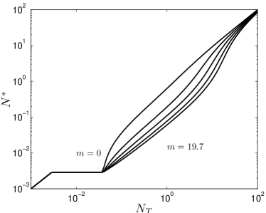
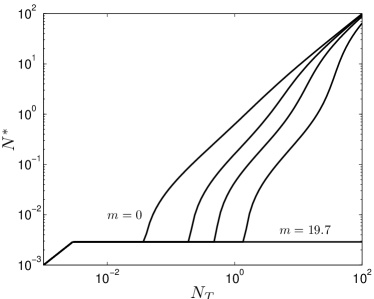
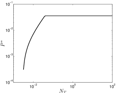
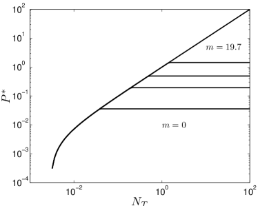
Refer to caption
Refer to caption
Refer to caption
Refer to caption
Refer to caption
Refer to caption
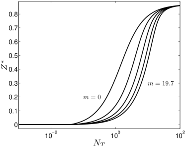
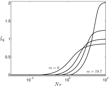
Figure 1: Equilibrium solutions as a function of total biomass for m=0,5,10,15,19.7𝑚05101519.7m=0,5,10,15,19.7 and R(P)=P/(P+0.159)𝑅𝑃𝑃𝑃0.159R(P)=P/(P+0.159). The left three are for δ0=0subscript𝛿00\delta_{0}=0 and the right three are for δ0=δsubscript𝛿0𝛿\delta_{0}=\delta. If E2subscript𝐸2E_{2} exists, it is the solution plotted. If E2subscript𝐸2E_{2} does not exist, but E1subscript𝐸1E_{1} does, then E1subscript𝐸1E_{1} is plotted. If neither exist, the limit point (NT,0,0)Tsuperscriptsubscript𝑁𝑇00𝑇(N_{T},0,0)^{T} is plotted

Figure 1 shows how the dominant equilibrium solutions change as the total biomass increases. We use parameter values given in Table 1, which were taken from [18]. We consider the case where R(P)=P/(P+0.159)𝑅𝑃𝑃𝑃0.159R(P)=P/(P+0.159) and various values of m𝑚m. The top three plots are for δ0=0subscript𝛿00\delta_{0}=0 and the bottom three are for δ0=δsubscript𝛿0𝛿\delta_{0}=\delta. We see that N=NTsuperscript𝑁subscript𝑁𝑇N^{*}=N_{T} and P=Z=0superscript𝑃superscript𝑍0P^{*}=Z^{*}=0 for NT<NT1subscript𝑁𝑇subscript𝑁𝑇1N_{T}<N_{T1} (e0subscript𝑒0e_{0} is plotted). Then for NT1<NT<NT2subscript𝑁𝑇1subscript𝑁𝑇subscript𝑁𝑇2N_{T1}<N_{T}<N_{T2} (E1subscript𝐸1E_{1} is plotted), Psuperscript𝑃P^{*} increases linearly with NTsubscript𝑁𝑇N_{T} while Nsuperscript𝑁N^{*} is fixed at NT1subscript𝑁𝑇1N_{T1} and Zsuperscript𝑍Z^{*} is fixed at 0. Then for NT>NT2subscript𝑁𝑇subscript𝑁𝑇2N_{T}>N_{T2} (E2subscript𝐸2E_{2} is plotted), Psuperscript𝑃P^{*} is fixed and Nsuperscript𝑁N^{*} and Zsuperscript𝑍Z^{*} increase with NTsubscript𝑁𝑇N_{T}, though Zsuperscript𝑍Z^{*} saturates and Nsuperscript𝑁N^{*} increases indefinitely. Note that NT2subscript𝑁𝑇2N_{T2} depends on m𝑚m when δ00subscript𝛿00\delta_{0}\neq 0, but not when δ0=0subscript𝛿00\delta_{0}=0. Also, Psuperscript𝑃P^{*} is independent of m𝑚m when δ0=0subscript𝛿00\delta_{0}=0, but changes for NT>NT2subscript𝑁𝑇subscript𝑁𝑇2N_{T}>N_{T2} when δ00subscript𝛿00\delta_{0}\neq 0. The value to which Zsuperscript𝑍Z^{*} saturates does not change with m𝑚m when δ0=0subscript𝛿00\delta_{0}=0, but increases with m𝑚m when δ00subscript𝛿00\delta_{0}\neq 0.

Parameter Value
μ𝜇\mu 5.95.95.9 day-1
λ𝜆\lambda 0.0170.0170.017 day-1
g𝑔g 777 day-1
γ𝛾\gamma 0.70.70.7
δ𝛿\delta 0.170.170.17 day-1
f(N)𝑓𝑁f(N) NN+k𝑁𝑁𝑘\frac{N}{N+k}
h(P)𝑃h(P) PP+K𝑃𝑃𝐾\frac{P}{P+K}
k𝑘k 1.0μM1.0𝜇M1.0\mu\mbox{M}
K𝐾K 1.0μM1.0𝜇M1.0\mu\mbox{M}
Table 1: Parameter values used for all computations

7 Linearization and Characteristic Equation

In this section, we will show that a general threshold delay equation and its corresponding delay differential equation, as in [19], have identical linearizations about an equilibrium solution.

Consider the threshold delay equation in the general form

(31) dx(t)dt=f(x(t),x(tτ(xt)),τ(xt)),τ(xt)0K(xt(u))𝑑u=m,formulae-sequence𝑑𝑥𝑡𝑑𝑡𝑓𝑥𝑡𝑥𝑡𝜏subscript𝑥𝑡𝜏subscript𝑥𝑡superscriptsubscript𝜏subscript𝑥𝑡0𝐾subscript𝑥𝑡𝑢differential-d𝑢𝑚\displaystyle\frac{dx(t)}{dt}=f(x(t),x(t-\tau(x_{t})),\tau(x_{t})),\hskip 14.22636pt\int_{-\tau(x_{t})}^{0}K(x_{t}(u))\,du=m,

and the corresponding functional differential equation

(32) dx^(t^)dt^=KK(x^(t^))f(x^(t^),x^(t^m/K),τ^(x^t^)),τ^(x^t^)=m/K0KK(x^t^(u))𝑑u,formulae-sequence𝑑^𝑥^𝑡𝑑^𝑡superscript𝐾𝐾^𝑥^𝑡𝑓^𝑥^𝑡^𝑥^𝑡𝑚superscript𝐾^𝜏subscript^𝑥^𝑡^𝜏subscript^𝑥^𝑡superscriptsubscript𝑚superscript𝐾0superscript𝐾𝐾subscript^𝑥^𝑡𝑢differential-d𝑢\displaystyle\frac{d\hat{x}(\hat{t})}{d\hat{t}}=\frac{K^{*}}{K(\hat{x}(\hat{t}))}f(\hat{x}(\hat{t}),\hat{x}(\hat{t}-m/K^{*}),\hat{\tau}(\hat{x}_{\hat{t}})),\hskip 14.22636pt\hat{\tau}(\hat{x}_{\hat{t}})=\int_{-m/K^{*}}^{0}\frac{K^{*}}{K(\hat{x}_{\hat{t}}(u))}\,du,

where f𝑓f and K𝐾K are differentiable, and Ksuperscript𝐾K^{*} is a typical value of K𝐾K. Results on the linearization of state-dependent delay differential equations with bounded delay can be found in [4]. These results apply to systems with bounded delay, which do not apply necessarily apply directly to the system here. Nevertheless, we will show that applying the linearization procedure for a state-dependent delay system with bounded delay to system (31) yields the same linearization as linearizing system (32) in the standard way for fixed delay systems.

Let xsuperscript𝑥x^{*} be an equilibrium solution of equations (31) and (32). That is, a constant function such that f(x,x,τ)=0𝑓superscript𝑥superscript𝑥superscript𝜏0f(x^{*},x^{*},\tau^{*})=0 where τ=m/K(x)=τ(x)=τ^(x)superscript𝜏𝑚𝐾superscript𝑥𝜏superscript𝑥^𝜏superscript𝑥\tau^{*}=m/K(x^{*})=\tau(x^{*})=\hat{\tau}(x^{*}). Let y(t)=x(t)x𝑦𝑡𝑥𝑡superscript𝑥y(t)=x(t)-x^{*}. By setting the state-dependent delay to its equilibrium value, and linearizing equation (31) as in [4], we obtain

dy(t)dt=𝑑𝑦𝑡𝑑𝑡absent\displaystyle\frac{dy(t)}{dt}= D1f(x,x,τ)y(t)+D2f(x,x,τ)y(tτ)subscript𝐷1𝑓superscript𝑥superscript𝑥superscript𝜏𝑦𝑡subscript𝐷2𝑓superscript𝑥superscript𝑥superscript𝜏𝑦𝑡superscript𝜏\displaystyle D_{1}f(x^{*},x^{*},\tau^{*})y(t)+D_{2}f(x^{*},x^{*},\tau^{*})y(t-\tau^{*})
(33) +D3f(x,x,τ)Dτ(x)ytsubscript𝐷3𝑓superscript𝑥superscript𝑥superscript𝜏𝐷𝜏superscript𝑥subscript𝑦𝑡\displaystyle+D_{3}f(x^{*},x^{*},\tau^{*})D\tau(x^{*})y_{t}

where Difsubscript𝐷𝑖𝑓D_{i}f is the derivative of f𝑓f with respect to its i𝑖ith argument and

(34) Dτ(x)yt=DK(x)K(x)τ0yt(u)𝑑u.𝐷𝜏superscript𝑥subscript𝑦𝑡𝐷𝐾superscript𝑥𝐾superscript𝑥superscriptsubscriptsuperscript𝜏0subscript𝑦𝑡𝑢differential-d𝑢\displaystyle D\tau(x^{*})y_{t}=-\frac{DK(x^{*})}{K(x^{*})}\int_{-\tau^{*}}^{0}y_{t}(u)\,du.

Let y^(t^)=x^(t^)x^𝑦^𝑡^𝑥^𝑡superscript𝑥\hat{y}(\hat{t})=\hat{x}(\hat{t})-x^{*}. Then linearizing equation (32) in the standard way yields

dy^(t^)dt^=𝑑^𝑦^𝑡𝑑^𝑡absent\displaystyle\frac{d\hat{y}(\hat{t})}{d\hat{t}}= KK(x)[D1f(x,x,τ)y^(t^)+D2f(x,x,τ)y^(t^m/K)\displaystyle\frac{K^{*}}{K(x^{*})}[D_{1}f(x^{*},x^{*},\tau^{*})\hat{y}(\hat{t})+D_{2}f(x^{*},x^{*},\tau^{*})\hat{y}(\hat{t}-m/K^{*})
(35) +D3f(x,x,τ)Dτ^(x)y^t^]\displaystyle+D_{3}f(x^{*},x^{*},\tau^{*})D\hat{\tau}(x^{*})\hat{y}_{\hat{t}}]

where

(36) Dτ^(x)y^t^=KDK(x)K(x)2m/K0y^t^(u)𝑑u.𝐷^𝜏superscript𝑥subscript^𝑦^𝑡superscript𝐾𝐷𝐾superscript𝑥𝐾superscriptsuperscript𝑥2superscriptsubscript𝑚superscript𝐾0subscript^𝑦^𝑡𝑢differential-d𝑢\displaystyle D\hat{\tau}(x^{*})\hat{y}_{\hat{t}}=-\frac{K^{*}DK(x^{*})}{K(x^{*})^{2}}\int_{-m/K^{*}}^{0}\hat{y}_{\hat{t}}(u)\,du.

Without any loss of generality, we can set K=K(x)superscript𝐾𝐾superscript𝑥K^{*}=K(x^{*}). Indeed, this would be the natural choice of Ksuperscript𝐾K^{*} if we were interested in solutions near a given equilibrium. Then it can be see that equations (7) and (7) are identical.

We can check that (34) is correct by verifying that

(37) limh0|τ(x+h)τ(x)+DK(x)K(x)τ0h(u)𝑑u|h=0,subscript0𝜏superscript𝑥𝜏superscript𝑥𝐷𝐾superscript𝑥𝐾superscript𝑥superscriptsubscriptsuperscript𝜏0𝑢differential-d𝑢norm0\displaystyle\lim_{h\rightarrow 0}\frac{\left|\tau(x^{*}+h)-\tau(x^{*})+\frac{DK(x^{*})}{K(x^{*})}\int_{-\tau^{*}}^{0}h(u)\,du\right|}{||h||}=0,

where h𝒞[r,0]𝒞𝑟0h\in\mathcal{C}[-r,0] for some r>τ(ϕ)𝑟𝜏italic-ϕr>\tau(\phi) for all ϕitalic-ϕ\phi in a neighbourhood of xsuperscript𝑥x^{*}. Here, ||.||||.|| is the usual sup norm. We proceed as follows:

|τ(x+h)τ(x)+DK(x)K(x)τ0h(u)𝑑u|𝜏superscript𝑥𝜏superscript𝑥𝐷𝐾superscript𝑥𝐾superscript𝑥superscriptsubscriptsuperscript𝜏0𝑢differential-d𝑢\displaystyle\left|\tau(x^{*}+h)-\tau(x^{*})+\frac{DK(x^{*})}{K(x^{*})}\int_{-\tau^{*}}^{0}h(u)\,du\right|
=\displaystyle= 1K(x)|τ(x+h)0K(x)𝑑uτ0K(x)𝑑u+DK(x)τ0h(u)𝑑u|.1𝐾superscript𝑥superscriptsubscript𝜏superscript𝑥0𝐾superscript𝑥differential-d𝑢superscriptsubscriptsuperscript𝜏0𝐾superscript𝑥differential-d𝑢𝐷𝐾superscript𝑥superscriptsubscriptsuperscript𝜏0𝑢differential-d𝑢\displaystyle\frac{1}{K(x^{*})}\left|\int_{-\tau(x^{*}+h)}^{0}K(x^{*})\,du-\int_{-\tau^{*}}^{0}K(x^{*})\,du+DK(x^{*})\int_{-\tau^{*}}^{0}h(u)\,du\right|.

Under the assumption that K𝒞1𝐾superscript𝒞1K\in\mathcal{C}^{1}, it is true that K(x)=K(x+x)DK(x)x+G(x)𝐾superscript𝑥𝐾superscript𝑥𝑥𝐷𝐾superscript𝑥𝑥𝐺𝑥K(x^{*})=K(x^{*}+x)-DK(x^{*})x+G(x), with G𝐺G satisfying

limx0|G(x)|xE=0,subscript𝑥0𝐺𝑥subscriptnorm𝑥𝐸0\displaystyle\lim_{x\rightarrow 0}\frac{|G(x)|}{||x||_{E}}=0,

where ||.||E||.||_{E} is the Euclidean norm on nsuperscript𝑛\mathbb{R}^{n}. Then

τ(x+h)0K(x)𝑑usuperscriptsubscript𝜏superscript𝑥0𝐾superscript𝑥differential-d𝑢\displaystyle\int_{-\tau(x^{*}+h)}^{0}K(x^{*})\,du
=\displaystyle= τ(x+h)0K(x+h(u))𝑑uDK(x)τ(x+h)0h(u)𝑑usuperscriptsubscript𝜏superscript𝑥0𝐾superscript𝑥𝑢differential-d𝑢𝐷𝐾superscript𝑥superscriptsubscript𝜏superscript𝑥0𝑢differential-d𝑢\displaystyle\int_{-\tau(x^{*}+h)}^{0}K(x^{*}+h(u))\,du-DK(x^{*})\int_{-\tau(x^{*}+h)}^{0}h(u)\,du
+τ(x+h)0G(h(u))𝑑u.superscriptsubscript𝜏superscript𝑥0𝐺𝑢differential-d𝑢\displaystyle+\int_{-\tau(x^{*}+h)}^{0}G(h(u))\,du.

Then by the definition of τ𝜏\tau:

τ(x+h)0K(x+h(u))𝑑u=τ0K(x)𝑑u=m.superscriptsubscript𝜏superscript𝑥0𝐾superscript𝑥𝑢differential-d𝑢superscriptsubscriptsuperscript𝜏0𝐾superscript𝑥differential-d𝑢𝑚\displaystyle\int_{-\tau(x^{*}+h)}^{0}K(x^{*}+h(u))\,du=\int_{-\tau^{*}}^{0}K(x^{*})\,du=m.

So it can then be seen that

limh0|τ(x+h)τ(x)+DK(x)K(x)τ(x)0h(u)𝑑u|hsubscript0𝜏superscript𝑥𝜏superscript𝑥𝐷𝐾superscript𝑥𝐾superscript𝑥superscriptsubscript𝜏superscript𝑥0𝑢differential-d𝑢norm\displaystyle\lim_{h\rightarrow 0}\frac{\left|\tau(x^{*}+h)-\tau(x^{*})+\frac{DK(x^{*})}{K(x^{*})}\int_{-\tau(x^{*})}^{0}h(u)\,du\right|}{||h||}
=\displaystyle= limh0|DK(x)ττ(x+h)h(u)𝑑u+τ(x+h)0G(h(u))𝑑u|K(x)hsubscript0𝐷𝐾superscript𝑥superscriptsubscriptsuperscript𝜏𝜏superscript𝑥𝑢differential-d𝑢superscriptsubscript𝜏superscript𝑥0𝐺𝑢differential-d𝑢𝐾superscript𝑥norm\displaystyle\lim_{h\rightarrow 0}\frac{\left|DK(x^{*})\int_{-\tau^{*}}^{-\tau(x^{*}+h)}h(u)\,du+\int_{-\tau(x^{*}+h)}^{0}G(h(u))\,du\right|}{K(x^{*})||h||}
=\displaystyle= 0,0\displaystyle 0,

from the properties of G𝐺G.

To verify equation (36), we check that

(38) limh0|τ^(x+h)τ^(x)+KDK(x)K(x)2m/K0h(u)𝑑u|h=0.subscript0^𝜏superscript𝑥^𝜏superscript𝑥superscript𝐾𝐷𝐾superscript𝑥𝐾superscriptsuperscript𝑥2superscriptsubscript𝑚superscript𝐾0𝑢differential-d𝑢norm0\displaystyle\lim_{h\rightarrow 0}\frac{\left|\hat{\tau}(x^{*}+h)-\hat{\tau}(x^{*})+\frac{K^{*}DK(x^{*})}{K(x^{*})^{2}}\int_{-m/K^{*}}^{0}h(u)\,du\right|}{||h||}=0.

This follows from the definition of τ^^𝜏\hat{\tau} in equation (32) and the fact that for x𝑥x near xsuperscript𝑥x^{*}

(39) 1K(x+x)=1K(x)DK(x)K(x)2x+G^(x),1𝐾superscript𝑥𝑥1𝐾superscript𝑥𝐷𝐾superscript𝑥𝐾superscriptsuperscript𝑥2𝑥^𝐺𝑥\displaystyle\frac{1}{K(x^{*}+x)}=\frac{1}{K(x^{*})}-\frac{DK(x^{*})}{K(x^{*})^{2}}x+\hat{G}(x),

for some function G^^𝐺\hat{G} that satisfies

limx0|G^(x)|xE=0.subscript𝑥0^𝐺𝑥subscriptnorm𝑥𝐸0\displaystyle\lim_{x\rightarrow 0}\frac{|\hat{G}(x)|}{||x||_{E}}=0.

In particular, the linearized system for our model ((15) or (22)) about an equilibrium solution (N,P,Z)Tsuperscriptsuperscript𝑁superscript𝑃superscript𝑍𝑇(N^{*},P^{*},Z^{*})^{T} with Rsuperscript𝑅R^{*} taken to be R(P)𝑅superscript𝑃R(P^{*}) is

(40) dy(t)dt=A1y(t)+A2y(tT)+A3T0y(t+u)𝑑u,𝑑𝑦𝑡𝑑𝑡subscript𝐴1𝑦𝑡subscript𝐴2𝑦𝑡𝑇subscript𝐴3superscriptsubscript𝑇0𝑦𝑡𝑢differential-d𝑢\displaystyle\frac{dy(t)}{dt}=A_{1}y(t)+A_{2}y(t-T)+A_{3}\int_{-T}^{0}y(t+u)\,du,

where

A1=(μPaδ0μc+λ+(1γ)gZbδ0δδ0+(1γ)gdμPaμcλgZbgd0eδ0TγgZdR(P)R(P)δ),subscript𝐴1𝜇superscript𝑃𝑎subscript𝛿0𝜇𝑐𝜆1𝛾𝑔superscript𝑍𝑏subscript𝛿0𝛿subscript𝛿01𝛾𝑔𝑑𝜇superscript𝑃𝑎𝜇𝑐𝜆𝑔superscript𝑍𝑏𝑔𝑑0superscript𝑒subscript𝛿0𝑇𝛾𝑔superscript𝑍𝑑superscript𝑅superscript𝑃𝑅superscript𝑃𝛿\displaystyle A_{1}=\left(\begin{array}[]{ccc}-\mu P^{*}a-\delta_{0}&-\mu c+\lambda+(1-\gamma)gZ^{*}b-\delta_{0}&\delta-\delta_{0}+(1-\gamma)gd\\ \mu P^{*}a&\mu c-\lambda-gZ^{*}b&-gd\\ 0&e^{-\delta_{0}T}\gamma gZ^{*}d\frac{R^{\prime}(P^{*})}{R(P^{*})}&-\delta\end{array}\right),
A2=(0000000eδ0TγgZ(bR(P)R(P)d)eδ0Tγgd),subscript𝐴20000000superscript𝑒subscript𝛿0𝑇𝛾𝑔superscript𝑍𝑏superscript𝑅superscript𝑃𝑅superscript𝑃𝑑superscript𝑒subscript𝛿0𝑇𝛾𝑔𝑑\displaystyle A_{2}=\left(\begin{array}[]{ccc}0&0&0\\ 0&0&0\\ 0&e^{-\delta_{0}T}\gamma gZ^{*}(b-\frac{R^{\prime}(P^{*})}{R(P^{*})}d)&e^{-\delta_{0}T}\gamma gd\end{array}\right),
A3=(0000000δ0eδ0TγgZdR(P)R(P)0),subscript𝐴30000000subscript𝛿0superscript𝑒subscript𝛿0𝑇𝛾𝑔superscript𝑍𝑑superscript𝑅superscript𝑃𝑅superscript𝑃0\displaystyle A_{3}=\left(\begin{array}[]{ccc}0&0&0\\ 0&0&0\\ 0&\delta_{0}e^{-\delta_{0}T}\gamma gZ^{*}d\frac{R^{\prime}(P^{*})}{R(P^{*})}&0\end{array}\right),

and a=f(N),b=h(P),c=f(N)formulae-sequence𝑎superscript𝑓superscript𝑁formulae-sequence𝑏superscriptsuperscript𝑃𝑐𝑓superscript𝑁a=f^{\prime}(N^{*}),b=h^{\prime}(P^{*}),c=f(N^{*}), d=h(P)𝑑superscript𝑃d=h(P^{*}), and T=m/R(P)=τ(m,P)=τ^(m,P)𝑇𝑚𝑅superscript𝑃𝜏𝑚superscript𝑃^𝜏𝑚superscript𝑃T=m/R(P^{*})=\tau(m,P^{*})=\hat{\tau}(m,P^{*}).

Substituting y(t)=vest𝑦𝑡𝑣superscript𝑒𝑠𝑡y(t)=ve^{st} into (40), with v3𝑣superscript3v\in\mathbb{R}^{3}, we can obtain the characteristic equation:

(41) det(sIA1A2esT+A3(1esT)s)=0.𝑠𝐼subscript𝐴1subscript𝐴2superscript𝑒𝑠𝑇subscript𝐴31superscript𝑒𝑠𝑇𝑠0\displaystyle\det\left(sI-A_{1}-A_{2}e^{-sT}+A_{3}\frac{(1-e^{-sT})}{s}\right)=0.

If all values of s𝑠s that satisfy equation (41) have a negative real part, then (N,P,Z)Tsuperscriptsuperscript𝑁superscript𝑃superscript𝑍𝑇(N^{*},P^{*},Z^{*})^{T} is an asymptotically stable equilibrium solution of system (22) [11]. Due to the equivalence of systems (15) and (22), they are asymptotically stable under identical conditions. Thus, we can use the characteristic equation (41) to obtain asymptotic stability in system (15). Therefore, if all values of s𝑠s that satisfy equation (41) have a negative real part, then (N,P,Z)Tsuperscriptsuperscript𝑁superscript𝑃superscript𝑍𝑇(N^{*},P^{*},Z^{*})^{T} is an asymptotically stable equilibrium solution of system (15).

8 Stability and Extinction

8.1 Conditions for the Extinction of Plankton

It is possible for the solutions to the TDE model (15) to approach the point e0=(NT,0,0)Tsubscript𝑒0superscriptsubscript𝑁𝑇00𝑇e_{0}=(N_{T},0,0)^{T}. To show this, we will use the following Lemma.

Lemma 8.1

If (N(t),P(t),Z(t))Tsuperscript𝑁𝑡𝑃𝑡𝑍𝑡𝑇(N(t),P(t),Z(t))^{T} is a solution to system (15) such that
limtP(t)=0subscript𝑡𝑃𝑡0\lim_{t\rightarrow\infty}P(t)=0, then limt(N(t),P(t),Z(t))T=(NT,0,0)Tsubscript𝑡superscript𝑁𝑡𝑃𝑡𝑍𝑡𝑇superscriptsubscript𝑁𝑇00𝑇\lim_{t\rightarrow\infty}(N(t),P(t),Z(t))^{T}=(N_{T},0,0)^{T}.

Proof: Assume that limtP(t)=0subscript𝑡𝑃𝑡0\lim_{t\rightarrow\infty}P(t)=0. The term eδ0τ(m,Pt)superscript𝑒subscript𝛿0𝜏𝑚subscript𝑃𝑡e^{-\delta_{0}\tau(m,P_{t})} is clearly bounded. Also, by Proposition 5.2, Z(tτ(m,Pt))<NT𝑍𝑡𝜏𝑚subscript𝑃𝑡subscript𝑁𝑇Z(t-\tau(m,P_{t}))<N_{T}, so this term is also bounded. From the properties of hh and R𝑅R in equations (4) and (5), there is a function, w𝑤w, such that limtw(t)=0subscript𝑡𝑤𝑡0\lim_{t\rightarrow\infty}w(t)=0 and dZ(t)dt<w(t)δZ(t)𝑑𝑍𝑡𝑑𝑡𝑤𝑡𝛿𝑍𝑡\frac{dZ(t)}{dt}<w(t)-\delta Z(t) for tt0𝑡subscript𝑡0t\geq t_{0}. Integrating this inequality, we obtain

Z(t)<eδ(tt0)Z(t0)+eδtt0teδuw(u)𝑑u.𝑍𝑡superscript𝑒𝛿𝑡subscript𝑡0𝑍subscript𝑡0superscript𝑒𝛿𝑡superscriptsubscriptsubscript𝑡0𝑡superscript𝑒𝛿𝑢𝑤𝑢differential-d𝑢\displaystyle Z(t)<e^{-\delta(t-t_{0})}Z(t_{0})+e^{-\delta t}\int_{t_{0}}^{t}e^{\delta u}w(u)\,du.

In the case where t0eδuw(u)𝑑u<superscriptsubscriptsubscript𝑡0superscript𝑒𝛿𝑢𝑤𝑢differential-d𝑢\int_{t_{0}}^{\infty}e^{\delta u}w(u)\,du<\infty it is obvious the final term approaches zero as t𝑡t\rightarrow\infty. Otherwise, we can apply l’Hôpital’s rule and get the same result. Since Z(t)>0𝑍𝑡0Z(t)>0 by Proposition 5.2, we have that limtZ(t)=0subscript𝑡𝑍𝑡0\lim_{t\rightarrow\infty}Z(t)=0.

The result then follows from the conservation law (3) if it is true that

limt0meδ0τ(s,Pt)γgZ(tτ(s,Pt))h(P(tτ(s,Pt)))R(P(tτ(s,Pt)))𝑑s=0.subscript𝑡superscriptsubscript0𝑚superscript𝑒subscript𝛿0𝜏𝑠subscript𝑃𝑡𝛾𝑔𝑍𝑡𝜏𝑠subscript𝑃𝑡𝑃𝑡𝜏𝑠subscript𝑃𝑡𝑅𝑃𝑡𝜏𝑠subscript𝑃𝑡differential-d𝑠0\displaystyle\lim_{t\rightarrow\infty}\int_{0}^{m}e^{-\delta_{0}\tau(s,P_{t})}\frac{\gamma gZ(t-\tau(s,P_{t}))h(P(t-\tau(s,P_{t})))}{R(P(t-\tau(s,P_{t})))}\,ds=0.

If limtτ(s,Pt)<subscript𝑡𝜏𝑠subscript𝑃𝑡\lim_{t\rightarrow\infty}\tau(s,P_{t})<\infty, then Z(tτ(s,Pt))0𝑍𝑡𝜏𝑠subscript𝑃𝑡0Z(t-\tau(s,P_{t}))\rightarrow 0 and the result immediately follows. If limtτ(s,Pt)=subscript𝑡𝜏𝑠subscript𝑃𝑡\lim_{t\rightarrow\infty}\tau(s,P_{t})=\infty then eδ0τ(s,Pt)0superscript𝑒subscript𝛿0𝜏𝑠subscript𝑃𝑡0e^{-\delta_{0}\tau(s,P_{t})}\rightarrow 0 and the result follows. \square

This also implies that if P^(t^)^𝑃^𝑡\hat{P}(\hat{t}) in the solution to the DDE model (22) reaches zero in finite time, then Z^(t^)^𝑍^𝑡\hat{Z}(\hat{t}) reaches zero at the same finite moment in time. This is because the transformation maps t=𝑡t=\infty to t^=w^<^𝑡^𝑤\hat{t}=\hat{w}<\infty.

The following Proposition shows conditions for the extinction of plankton.

Proposition 8.2

If 0<NT<NT10subscript𝑁𝑇subscript𝑁𝑇10<N_{T}<N_{T1}, where NT1subscript𝑁𝑇1N_{T1} is given in (29), and (ϕ1,ϕ2,ϕ3)TDNTsuperscriptsubscriptitalic-ϕ1subscriptitalic-ϕ2subscriptitalic-ϕ3𝑇subscript𝐷subscript𝑁𝑇(\phi_{1},\phi_{2},\phi_{3})^{T}\in D_{N_{T}}, then the solution to the initial value problem (14)-(15) asymptotically approaches (NT,0,0)Tsuperscriptsubscript𝑁𝑇00𝑇(N_{T},0,0)^{T}.

Proof: From (15b), we have that dPdt<μf(NT)P(t)λP(t)𝑑𝑃𝑑𝑡𝜇𝑓subscript𝑁𝑇𝑃𝑡𝜆𝑃𝑡\frac{dP}{dt}<\mu f(N_{T})P(t)-\lambda P(t). Then NT<NT1subscript𝑁𝑇subscript𝑁𝑇1N_{T}<N_{T1} implies that μf(NT)λ<0𝜇𝑓subscript𝑁𝑇𝜆0\mu f(N_{T})-\lambda<0, which implies that P(t)<P(t0)e(μf(NT)λ)(tt0)𝑃𝑡𝑃subscript𝑡0superscript𝑒𝜇𝑓subscript𝑁𝑇𝜆𝑡subscript𝑡0P(t)<P(t_{0})e^{(\mu f(N_{T})-\lambda)(t-t_{0})}. Since P(t)>0𝑃𝑡0P(t)>0 from Proposition 5.2, limtP(t)=0subscript𝑡𝑃𝑡0\lim_{t\rightarrow\infty}P(t)=0. The result then follows from Lemma 8.1. \square

8.2 Global Stability of E1subscript𝐸1E_{1}

Here we will show conditions for the global stability of E1subscript𝐸1E_{1}. Consider the following Lemma.

Lemma 8.3

Let (ϕ1,ϕ2,ϕ3)TDNTsuperscriptsubscriptitalic-ϕ1subscriptitalic-ϕ2subscriptitalic-ϕ3𝑇subscript𝐷subscript𝑁𝑇(\phi_{1},\phi_{2},\phi_{3})^{T}\in D_{N_{T}} and denote (N,P,Z)T:[0,)3:superscript𝑁𝑃𝑍𝑇0superscript3(N,P,Z)^{T}:[0,\infty)\rightarrow\mathbb{R}^{3} as the solution to the initial value problem (14)-(15). If NT>NT1subscript𝑁𝑇subscript𝑁𝑇1N_{T}>N_{T1}, then for any constant β>NTNT1𝛽subscript𝑁𝑇subscript𝑁𝑇1\beta>N_{T}-N_{T1}, there exists a t1t0subscript𝑡1subscript𝑡0t_{1}\geq t_{0} such that P(t)<β𝑃𝑡𝛽P(t)<\beta for all tt1𝑡subscript𝑡1t\geq t_{1}.

Proof: Fix β<NTNT1𝛽subscript𝑁𝑇subscript𝑁𝑇1\beta<N_{T}-N_{T1}. From the conservation law (3) and Proposition 5.2, N(t)<NTP(t)𝑁𝑡subscript𝑁𝑇𝑃𝑡N(t)<N_{T}-P(t). Then for P(t)β𝑃𝑡𝛽P(t)\geq\beta we have

dP(t)dt𝑑𝑃𝑡𝑑𝑡\displaystyle\frac{dP(t)}{dt} <[μf(N(t))λ]P(t),absentdelimited-[]𝜇𝑓𝑁𝑡𝜆𝑃𝑡\displaystyle<[\mu f(N(t))-\lambda]P(t),
<[μf(NTP(t))λ]P(t),absentdelimited-[]𝜇𝑓subscript𝑁𝑇𝑃𝑡𝜆𝑃𝑡\displaystyle<[\mu f(N_{T}-P(t))-\lambda]P(t),
<[μf(NTβ)λ]P(t).absentdelimited-[]𝜇𝑓subscript𝑁𝑇𝛽𝜆𝑃𝑡\displaystyle<[\mu f(N_{T}-\beta)-\lambda]P(t).

Since μf(NTβ)λ<μf(NT1)λ=0𝜇𝑓subscript𝑁𝑇𝛽𝜆𝜇𝑓subscript𝑁𝑇1𝜆0\mu f(N_{T}-\beta)-\lambda<\mu f(N_{T1})-\lambda=0, we have

dP(t)dt𝑑𝑃𝑡𝑑𝑡\displaystyle\frac{dP(t)}{dt} <[μf(NTβ)λ]βabsentdelimited-[]𝜇𝑓subscript𝑁𝑇𝛽𝜆𝛽\displaystyle<[\mu f(N_{T}-\beta)-\lambda]\beta

for P(t)β𝑃𝑡𝛽P(t)\geq\beta. Therefore there exists t1t0subscript𝑡1subscript𝑡0t_{1}\geq t_{0} such that P(t)<β𝑃𝑡𝛽P(t)<\beta for all tt1𝑡subscript𝑡1t\geq t_{1}. \square

Proposition 8.4

Let (ϕ1,ϕ2,ϕ3)TDNTsuperscriptsubscriptitalic-ϕ1subscriptitalic-ϕ2subscriptitalic-ϕ3𝑇subscript𝐷subscript𝑁𝑇(\phi_{1},\phi_{2},\phi_{3})^{T}\in D_{N_{T}} and denote (N,P,Z)T:[0,)3:superscript𝑁𝑃𝑍𝑇0superscript3(N,P,Z)^{T}:[0,\infty)\rightarrow\mathbb{R}^{3} as the solution to the initial value problem (14)-(15). If NT1<NT<NT2subscript𝑁𝑇1subscript𝑁𝑇subscript𝑁𝑇2N_{T1}<N_{T}<N_{T2}, then limt(N(t),P(t),Z(t))T=(N1,P1,0)Tsubscript𝑡superscript𝑁𝑡𝑃𝑡𝑍𝑡𝑇superscriptsuperscriptsubscript𝑁1superscriptsubscript𝑃10𝑇\lim_{t\rightarrow\infty}(N(t),P(t),Z(t))^{T}=(N_{1}^{*},P_{1}^{*},0)^{T}.

Proof: Note that μf(N1)λ=0𝜇𝑓superscriptsubscript𝑁1𝜆0\mu f(N_{1}^{*})-\lambda=0 and P1=NTN1<P2superscriptsubscript𝑃1subscript𝑁𝑇superscriptsubscript𝑁1superscriptsubscript𝑃2P_{1}^{*}=N_{T}-N_{1}^{*}<P_{2}^{*} for NT<NT2subscript𝑁𝑇subscript𝑁𝑇2N_{T}<N_{T2}. Consider the function

V1(t)=N1N(t)[μf(x)λ]𝑑x+δ0NTN1P(t)x+N1NTx𝑑x.subscript𝑉1𝑡superscriptsubscriptsuperscriptsubscript𝑁1𝑁𝑡delimited-[]𝜇𝑓𝑥𝜆differential-d𝑥subscript𝛿0superscriptsubscriptsubscript𝑁𝑇superscriptsubscript𝑁1𝑃𝑡𝑥superscriptsubscript𝑁1subscript𝑁𝑇𝑥differential-d𝑥\displaystyle V_{1}(t)=\int_{N_{1}^{*}}^{N(t)}[\mu f(x)-\lambda]\,dx+\delta_{0}\int_{N_{T}-N_{1}^{*}}^{P(t)}\frac{x+N_{1}^{*}-N_{T}}{x}\,dx.

We have that V1(t)0subscript𝑉1𝑡0V_{1}(t)\geq 0 for P(t)>0𝑃𝑡0P(t)>0. Taking the derivative along solutions to the TDE model (15), we obtain

ddtV1(t)=𝑑𝑑𝑡subscript𝑉1𝑡absent\displaystyle\frac{d}{dt}V_{1}(t)= [μf(N(t))λ][μP(t)f(N(t))+λP(t)+δZ(t)+(1γ)gZ(t)h(P(t))\displaystyle[\mu f(N(t))-\lambda][-\mu P(t)f(N(t))+\lambda P(t)+\delta Z(t)+(1-\gamma)gZ(t)h(P(t))
+δ0(NTN(t)P(t)Z(t))]\displaystyle+\delta_{0}(N_{T}-N(t)-P(t)-Z(t))]
+δ0P(t)+N1NTP(t)[μP(t)f(N(t))λP(t)gZ(t)h(P(t))],subscript𝛿0𝑃𝑡superscriptsubscript𝑁1subscript𝑁𝑇𝑃𝑡delimited-[]𝜇𝑃𝑡𝑓𝑁𝑡𝜆𝑃𝑡𝑔𝑍𝑡𝑃𝑡\displaystyle+\delta_{0}\frac{P(t)+N_{1}^{*}-N_{T}}{P(t)}[\mu P(t)f(N(t))-\lambda P(t)-gZ(t)h(P(t))],
\displaystyle\leq P(t)[μf(N(t))λ]2δ0[N(t)N1][μf(N(t))λ]+MZ(t),𝑃𝑡superscriptdelimited-[]𝜇𝑓𝑁𝑡𝜆2subscript𝛿0delimited-[]𝑁𝑡superscriptsubscript𝑁1delimited-[]𝜇𝑓𝑁𝑡𝜆𝑀𝑍𝑡\displaystyle-P(t)[\mu f(N(t))-\lambda]^{2}-\delta_{0}[N(t)-N_{1}^{*}][\mu f(N(t))-\lambda]+MZ(t),

for some positive constant M𝑀M. This M𝑀M exists because N(t)𝑁𝑡N(t) and P(t)𝑃𝑡P(t) are bounded and from the properties of hh in (4). Then consider the function

V2(t)=Z(t)+tτ(m,Pt)tγgeδ0τ(m,β)Z(u)h(P(u))𝑑u.subscript𝑉2𝑡𝑍𝑡superscriptsubscript𝑡𝜏𝑚subscript𝑃𝑡𝑡𝛾𝑔superscript𝑒subscript𝛿0𝜏𝑚𝛽𝑍𝑢𝑃𝑢differential-d𝑢\displaystyle V_{2}(t)=Z(t)+\int_{t-\tau(m,P_{t})}^{t}\gamma ge^{-\delta_{0}\tau(m,\beta)}Z(u)h(P(u))\,du.

We have that V2(t)0subscript𝑉2𝑡0V_{2}(t)\geq 0. Choose β(NTNT1,P2)𝛽subscript𝑁𝑇subscript𝑁𝑇1superscriptsubscript𝑃2\beta\in(N_{T}-N_{T1},P_{2}^{*}). Then by Lemma 8.3, there exists t1t0subscript𝑡1subscript𝑡0t_{1}\geq t_{0} such that P(t)<β𝑃𝑡𝛽P(t)<\beta for tt1𝑡subscript𝑡1t\geq t_{1}. This implies that

γgeδ0τ(m,Pt)h(P(t))<γgeδ0τ(m,β)h(β)<γgeδ0τ(m,P2)h(P2)=δ𝛾𝑔superscript𝑒subscript𝛿0𝜏𝑚subscript𝑃𝑡𝑃𝑡𝛾𝑔superscript𝑒subscript𝛿0𝜏𝑚𝛽𝛽𝛾𝑔superscript𝑒subscript𝛿0𝜏𝑚superscriptsubscript𝑃2superscriptsubscript𝑃2𝛿\displaystyle\gamma ge^{-\delta_{0}\tau(m,P_{t})}h(P(t))<\gamma ge^{-\delta_{0}\tau(m,\beta)}h(\beta)<\gamma ge^{-\delta_{0}\tau(m,P_{2}^{*})}h(P_{2}^{*})=\delta

for tt1𝑡subscript𝑡1t\geq t_{1}. Define the positive constant α=δγgeδ0τ(m,β)h(β)𝛼𝛿𝛾𝑔superscript𝑒subscript𝛿0𝜏𝑚𝛽𝛽\alpha=\delta-\gamma ge^{-\delta_{0}\tau(m,\beta)}h(\beta). Differentiating, we have that

ddtV2(t)=𝑑𝑑𝑡subscript𝑉2𝑡absent\displaystyle\frac{d}{dt}V_{2}(t)= R(P(t))eδ0τ(m,Pt)γgZ(tτ(m,Pt))h(P(tτ(m,Pt)))R(P(tτ(m,Pt)))δZ(t)𝑅𝑃𝑡superscript𝑒subscript𝛿0𝜏𝑚subscript𝑃𝑡𝛾𝑔𝑍𝑡𝜏𝑚subscript𝑃𝑡𝑃𝑡𝜏𝑚subscript𝑃𝑡𝑅𝑃𝑡𝜏𝑚subscript𝑃𝑡𝛿𝑍𝑡\displaystyle R(P(t))e^{-\delta_{0}\tau(m,P_{t})}\frac{\gamma gZ(t-\tau(m,P_{t}))h(P(t-\tau(m,P_{t})))}{R(P(t-\tau(m,P_{t})))}-\delta Z(t)
+γgeδ0τ(m,β)Z(t)h(P(t))𝛾𝑔superscript𝑒subscript𝛿0𝜏𝑚𝛽𝑍𝑡𝑃𝑡\displaystyle+\gamma ge^{-\delta_{0}\tau(m,\beta)}Z(t)h(P(t))
γgeδ0τ(m,β)Z(tτ(m,Pt)h(P(tτ(m,Pt))(1τt),\displaystyle-\gamma ge^{-\delta_{0}\tau(m,\beta)}Z(t-\tau(m,P_{t})h(P(t-\tau(m,P_{t}))\left(1-\frac{\partial\tau}{\partial t}\right),
\displaystyle\leq αZ(t),𝛼𝑍𝑡\displaystyle-\alpha Z(t),

where we have used that

1τt=R(P(t))R(P(tτ(m,Pt)),\displaystyle 1-\frac{\partial\tau}{\partial t}=\frac{R(P(t))}{R(P(t-\tau(m,P_{t}))},

h(P(t))<h(β)𝑃𝑡𝛽h(P(t))<h(\beta), and eδ0τ(m,Pt)<eδ0τ(m,β)superscript𝑒subscript𝛿0𝜏𝑚subscript𝑃𝑡superscript𝑒subscript𝛿0𝜏𝑚𝛽e^{-\delta_{0}\tau(m,P_{t})}<e^{-\delta_{0}\tau(m,\beta)} for tt1𝑡subscript𝑡1t\geq t_{1}. Setting V(t)=V1(t)+M+M1αV2(t)𝑉𝑡subscript𝑉1𝑡𝑀subscript𝑀1𝛼subscript𝑉2𝑡V(t)=V_{1}(t)+\frac{M+M_{1}}{\alpha}V_{2}(t) where M1>0subscript𝑀10M_{1}>0, we have that V(t)0𝑉𝑡0V(t)\geq 0 and that

ddtV(t)δ0[N(t)N1][μf(N(t))λ]M1Z(t),𝑑𝑑𝑡𝑉𝑡subscript𝛿0delimited-[]𝑁𝑡superscriptsubscript𝑁1delimited-[]𝜇𝑓𝑁𝑡𝜆subscript𝑀1𝑍𝑡\displaystyle\frac{d}{dt}V(t)\leq-\delta_{0}[N(t)-N_{1}^{*}][\mu f(N(t))-\lambda]-M_{1}Z(t),

for tt1𝑡subscript𝑡1t\geq t_{1}. Integrating, we obtain that

(42) V(t)+t1t[δ0(N(u)N1)(μf(N(u))λ)+M1Z(u)]𝑑uV(t1).𝑉𝑡superscriptsubscriptsubscript𝑡1𝑡delimited-[]subscript𝛿0𝑁𝑢superscriptsubscript𝑁1𝜇𝑓𝑁𝑢𝜆subscript𝑀1𝑍𝑢differential-d𝑢𝑉subscript𝑡1\displaystyle V(t)+\int_{t_{1}}^{t}[\delta_{0}(N(u)-N_{1}^{*})(\mu f(N(u))-\lambda)+M_{1}Z(u)]\,du\leq V(t_{1}).

Since V(t)𝑉𝑡V(t) and the above integrand are nonnegative, and since the inequality (42) must be true for all time, it follows that

t0[δ0(N(u)N1)(μf(N(u))λ)+M1Z(u)]𝑑u<.superscriptsubscriptsubscript𝑡0delimited-[]subscript𝛿0𝑁𝑢superscriptsubscript𝑁1𝜇𝑓𝑁𝑢𝜆subscript𝑀1𝑍𝑢differential-d𝑢\displaystyle\int_{t_{0}}^{\infty}[\delta_{0}(N(u)-N_{1}^{*})(\mu f(N(u))-\lambda)+M_{1}Z(u)]\,du<\infty.

By Barbălat’s Lemma [8], it must be true that N(t)N1𝑁𝑡superscriptsubscript𝑁1N(t)\rightarrow N_{1}^{*} and Z(t)0𝑍𝑡0Z(t)\rightarrow 0. By the conservation law (3) it then follows that P(t)P1𝑃𝑡superscriptsubscript𝑃1P(t)\rightarrow P_{1}^{*}. \square

The attractivity of E1subscript𝐸1E_{1} has thus been shown. However, Proposition 8.4 does not address its stability. Let (N,P,Z)T:[0,)3:superscript𝑁𝑃𝑍𝑇0superscript3(N,P,Z)^{T}:[0,\infty)\rightarrow\mathbb{R}^{3} denote the solution to the initial value problem (14) - (15). We will consider an equilibrium point E𝐸E to be asymptotically stable if for any ε>0𝜀0\varepsilon>0, there exists a neighbourhood Nεsubscript𝑁𝜀N_{\varepsilon} around E𝐸E such that if (ϕ1,ϕ2,ϕ3)DNTNεsubscriptitalic-ϕ1subscriptitalic-ϕ2subscriptitalic-ϕ3subscript𝐷subscript𝑁𝑇subscript𝑁𝜀(\phi_{1},\phi_{2},\phi_{3})\in D_{N_{T}}\cap N_{\varepsilon} then (N(t),P(t),Z(t))TE<εnormsuperscript𝑁𝑡𝑃𝑡𝑍𝑡𝑇𝐸𝜀||(N(t),P(t),Z(t))^{T}-E||<\varepsilon for tt0𝑡subscript𝑡0t\geq t_{0} and limt(N(t),P(t),Z(t))T=Esubscript𝑡superscript𝑁𝑡𝑃𝑡𝑍𝑡𝑇𝐸\lim_{t\rightarrow\infty}(N(t),P(t),Z(t))^{T}=E.

We will use the linearization of the TDE model (15) to prove the following Proposition.

Proposition 8.5

If NT1<NT<NT2subscript𝑁𝑇1subscript𝑁𝑇subscript𝑁𝑇2N_{T1}<N_{T}<N_{T2}, then E1subscript𝐸1E_{1} is asymptotically stable.

Proof: The condition NT1<NTsubscript𝑁𝑇1subscript𝑁𝑇N_{T1}<N_{T} ensures that E1=(N1,P1,0)Tsubscript𝐸1superscriptsuperscriptsubscript𝑁1superscriptsubscript𝑃10𝑇E_{1}=(N_{1}^{*},P_{1}^{*},0)^{T} exists. The characteristic equation of the corresponding linear system is

det(s+μP1a+δ0δ0δ+δ0(1γ)gdμP1asgd00s+δγgde(δ0+s)T)𝑠𝜇superscriptsubscript𝑃1𝑎subscript𝛿0subscript𝛿0𝛿subscript𝛿01𝛾𝑔𝑑𝜇superscriptsubscript𝑃1𝑎𝑠𝑔𝑑00𝑠𝛿𝛾𝑔𝑑superscript𝑒subscript𝛿0𝑠𝑇\displaystyle\det\left(\begin{array}[]{ccc}s+\mu P_{1}^{*}a+\delta_{0}&\delta_{0}&-\delta+\delta_{0}-(1-\gamma)gd\\ -\mu P_{1}^{*}a&s&gd\\ 0&0&s+\delta-\gamma gde^{-(\delta_{0}+s)T}\end{array}\right)
=(s+μP1a)(s+δ0)(s+δγgde(δ0+s)T)=0.absent𝑠𝜇superscriptsubscript𝑃1𝑎𝑠subscript𝛿0𝑠𝛿𝛾𝑔𝑑superscript𝑒subscript𝛿0𝑠𝑇0\displaystyle=(s+\mu P_{1}^{*}a)(s+\delta_{0})(s+\delta-\gamma gde^{-(\delta_{0}+s)T})=0.

The first two factors give two negative real eigenvalues. Since NT<NT2subscript𝑁𝑇subscript𝑁𝑇2N_{T}<N_{T2}, it is true that γgdeδ0T<δ𝛾𝑔𝑑superscript𝑒subscript𝛿0𝑇𝛿\gamma gde^{-\delta_{0}T}<\delta. Set s=α+iω𝑠𝛼𝑖𝜔s=\alpha+i\omega for real α𝛼\alpha and ω𝜔\omega and assume that α0𝛼0\alpha\geq 0. We have that s+δγgde(δ0+s)T=0𝑠𝛿𝛾𝑔𝑑superscript𝑒subscript𝛿0𝑠𝑇0s+\delta-\gamma gde^{-(\delta_{0}+s)T}=0 if and only if α+iω+δ=γgde(δ0+α+iω)T𝛼𝑖𝜔𝛿𝛾𝑔𝑑superscript𝑒subscript𝛿0𝛼𝑖𝜔𝑇\alpha+i\omega+\delta=\gamma gde^{-(\delta_{0}+\alpha+i\omega)T}. Squaring the modulus of both sides we obtain

(α+δ)2+ω2=(γgd)2e2(δ0+α)T<δ2,superscript𝛼𝛿2superscript𝜔2superscript𝛾𝑔𝑑2superscript𝑒2subscript𝛿0𝛼𝑇superscript𝛿2\displaystyle(\alpha+\delta)^{2}+\omega^{2}=(\gamma gd)^{2}e^{-2(\delta_{0}+\alpha)T}<\delta^{2},

which implies α<0𝛼0\alpha<0. This contradiction shows that there are no solutions with nonnegative real part. Since all the eigenvalues have negative real parts, E1subscript𝐸1E_{1} is asymptotically stable. \square The global attractivity together with the local stability of E1subscript𝐸1E_{1} for NT1<NT<NT2subscript𝑁𝑇1subscript𝑁𝑇subscript𝑁𝑇2N_{T1}<N_{T}<N_{T2} shows that E1subscript𝐸1E_{1} is globally asymptotically stable on DNTsubscript𝐷subscript𝑁𝑇D_{N_{T}}.

8.3 Stability of E2subscript𝐸2E_{2}: No Delay

If m=0𝑚0m=0 then the zooplankton are considered mature immediately at birth. In this case there is no delay and system (15) is just a system of ordinary differential equations. In [13], we showed that if hh has a negative second derivative (a Type II response) and f𝑓f has a negative second derivative, which is the case we will consider in the following sections, there is a unique NT3>NT2subscript𝑁𝑇3subscript𝑁𝑇2N_{T3}>N_{T2} such that E2subscript𝐸2E_{2} is asymptotically stable if NT2<NT<NT3subscript𝑁𝑇2subscript𝑁𝑇subscript𝑁𝑇3N_{T2}<N_{T}<N_{T3} and unstable if NT>NT3subscript𝑁𝑇subscript𝑁𝑇3N_{T}>N_{T3}. This value of NT3subscript𝑁𝑇3N_{T3} is independent of δ0subscript𝛿0\delta_{0} and the functional form of R(P)𝑅𝑃R(P), since m=0𝑚0m=0 implies that δ0subscript𝛿0\delta_{0} and R(P)𝑅𝑃R(P) do not play a role in system (15) under the assumption that (ϕ1,ϕ2,ϕ3)DNTsubscriptitalic-ϕ1subscriptitalic-ϕ2subscriptitalic-ϕ3subscript𝐷subscript𝑁𝑇(\phi_{1},\phi_{2},\phi_{3})\in D_{N_{T}}.

8.4 Stability of E2subscript𝐸2E_{2}: State-Independent Delay

Consider the case where R(P)𝑅𝑃R(P) is constant. That is, the growth rate of zooplankton is independent of the phytoplankton population. Without loss of generality, we will assume m𝑚m has been scaled so that R(P)=1𝑅𝑃1R(P)=1. In this sense, m𝑚m has dimensions of time, and represents the age at which zooplankton reaches maturity. In this case, the delay is no longer state-dependent and is fixed at τ=m𝜏𝑚\tau=m.

Due to the complicated nature of the resulting characteristic equation, we use numerical methods to study the stability of E2subscript𝐸2E_{2} (both here in the state-independent delay case and in the following section, which deals with the state-dependent delay problem). We use the parameter values in Table 1.

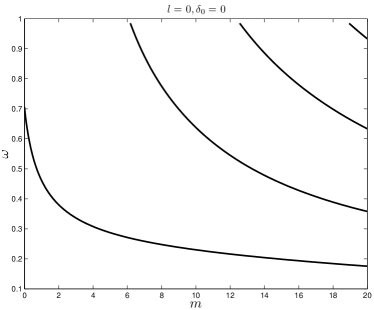
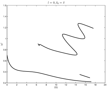
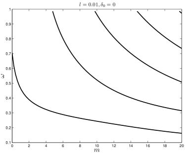
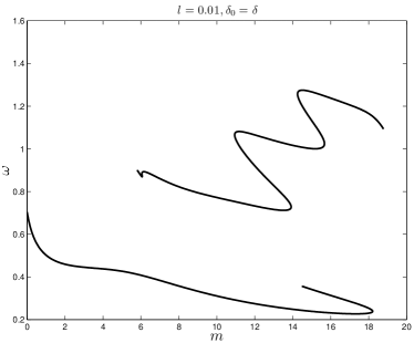
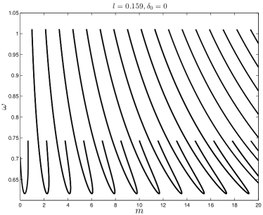
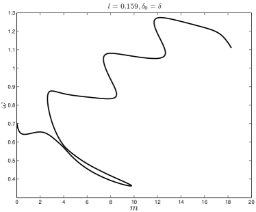
By setting s=iω𝑠𝑖𝜔s=i\omega in the characteristic equation (41) and allowing the m𝑚m and NTsubscript𝑁𝑇N_{T} parameters to vary, we can find solutions where the eigenvalues have zero real part. These represent critical points where stability might switch. Since the characteristic equation is complex valued, it gives us two equations that need to be satisfied. The equilibrium equations change with changing m𝑚m and NTsubscript𝑁𝑇N_{T}, so (28) gives us three more equations to solve. We then have six unknowns: N,P,Z,m,NT,ωsuperscript𝑁superscript𝑃superscript𝑍𝑚subscript𝑁𝑇𝜔N^{*},P^{*},Z^{*},m,N_{T},\omega. We can then find one-dimensional curves where the five equations are satisfied, using pseudo-arclength continuation [9]. Note that if (N,P,Z,m,NT,ω)superscript𝑁superscript𝑃superscript𝑍𝑚subscript𝑁𝑇𝜔(N^{*},P^{*},Z^{*},m,N_{T},\omega) solves the five equations then ω𝜔\omega represents the frequency for solutions to system (15) near the corresponding equilibrium solution (N,P,Z)superscript𝑁superscript𝑃superscript𝑍(N^{*},P^{*},Z^{*}) when the size at which the immature zooplankton reach maturity is m𝑚m and the total biomass is NTsubscript𝑁𝑇N_{T}.

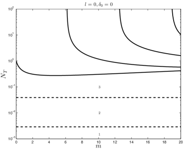
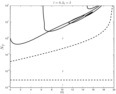
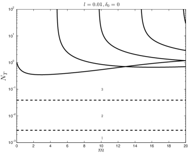
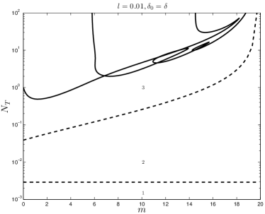
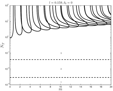
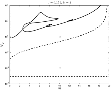
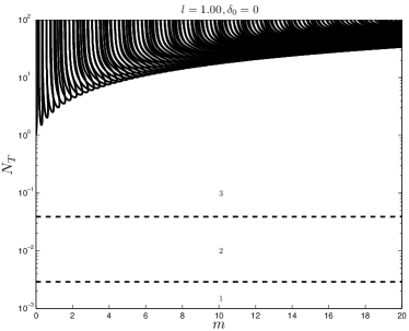
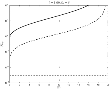
Figure 2 shows regions in the mNT𝑚subscript𝑁𝑇m-N_{T} plane where the equilibrium solutions exhibit different behaviour. This was done for two cases: δ0=0subscript𝛿00\delta_{0}=0 (left in Figure 2) and δ0=δsubscript𝛿0𝛿\delta_{0}=\delta (right in Figure 2). The former case represents the situation where the immature zooplankton have a zero death rate. That is, we ignore the possibility of them dying before reaching maturity. In region 1 we have that E1subscript𝐸1E_{1} and E2subscript𝐸2E_{2} do not exist. This region is the same, regardless of the value of δ0subscript𝛿0\delta_{0}. In region 2, E1subscript𝐸1E_{1} exists, but E2subscript𝐸2E_{2} does not. This region does depend on the value of δ0subscript𝛿0\delta_{0}, as a larger δ0subscript𝛿0\delta_{0} requires more biomass for the E2subscript𝐸2E_{2} equilibrium to exist. Region 3 shows where E1subscript𝐸1E_{1} and E2subscript𝐸2E_{2} exist. We note that Rln(γg/δ)/δ019.77subscript𝑅𝛾𝑔𝛿subscript𝛿019.77R_{\infty}\ln(\gamma g/\delta)/\delta_{0}\approx 19.77, which is an upper limit for m𝑚m when δ0>0subscript𝛿00\delta_{0}>0. The solid curves shows the values of m𝑚m and NTsubscript𝑁𝑇N_{T} where the linearized system has an eigenvalue with zero real part. The subset of region 3 below the solid curves represents values of m𝑚m and NTsubscript𝑁𝑇N_{T} where the E2subscript𝐸2E_{2} equilibrium is asymptotically stable. This follows from the continuity of the eigenvalues with respect to parameter values and the fact that there are no eigenvalues with nonnegative real parts when m=0𝑚0m=0 and NT2<NT<NT3subscript𝑁𝑇2subscript𝑁𝑇subscript𝑁𝑇3N_{T2}<N_{T}<N_{T3} (between where the upper dotted curve intersects the vertical axis and where the solid curve intersects the vertical axis).

These regions are all fairly independent of m𝑚m when δ0=0subscript𝛿00\delta_{0}=0. That is, if the juvenile zooplankton have a zero death rate, then the required level of maturity has little effect on the stability of the equilibrium solutions. However, when there is positive death rate for the immature zooplankton, the required level of maturity plays a more important role. We see that critical values of total biomass increase with increasing m𝑚m.

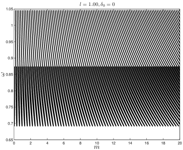
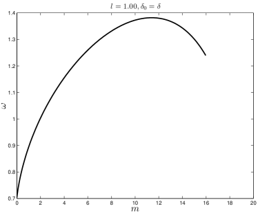
Figure 3 shows the frequencies that correspond to the curves in Figure 2. These are the imaginary parts of the eigenvalues with zero real parts along the curves. For values of m𝑚m and NTsubscript𝑁𝑇N_{T} near the solid curves in Figure 2, we would expect a slow growth or decay rate in the solution to system (15) when it is near the equilibrium solution, and for it to have a frequency close to the corresponding value of ω𝜔\omega in Figure 3.

Refer to caption
Refer to caption
Figure 2: The solid curves are where the linearized system has an eigenvalue with zero real part for R(P)=1𝑅𝑃1R(P)=1 and δ0=0subscript𝛿00\delta_{0}=0 (left) and δ0=δsubscript𝛿0𝛿\delta_{0}=\delta (right). Region 1 is where E1subscript𝐸1E_{1} and E2subscript𝐸2E_{2} do not exist. Region 2 is where E1subscript𝐸1E_{1} exists, but E2subscript𝐸2E_{2} does not. Region 3 is where E1subscript𝐸1E_{1} and E2subscript𝐸2E_{2} exist. The subset of region 3 under the solid curves is where E2subscript𝐸2E_{2} is asymptotically stable
Refer to caption
Refer to caption
Figure 3: The corresponding frequencies to the curves in Figure 2. The value of ω𝜔\omega is the imaginary part of the eigenvalue with zero real part along these curves

8.5 Stability of E2subscript𝐸2E_{2}: State-Dependent Delay

Here we consider the case where R(P)=PP+l𝑅𝑃𝑃𝑃𝑙R(P)=\frac{P}{P+l} for various values of l𝑙l. Using the same numerical technique as in the previous section, we compute curves in the mNT𝑚subscript𝑁𝑇m-N_{T} plane where there is an eigenvalue with zero real part. This tells us parameter values where stability can change.

Figure 4 shows regions in the mNT𝑚subscript𝑁𝑇m-N_{T} plane that have different behaviour. This was done for δ0=0subscript𝛿00\delta_{0}=0 (left figures), δ0=δsubscript𝛿0𝛿\delta_{0}=\delta (right figures) and for l=0.01𝑙0.01l=0.01 (top figures), l=0.159𝑙0.159l=0.159 (figures second from the top), l=1.00𝑙1.00l=1.00 (bottom figures). As before, region 1 is where neither E1subscript𝐸1E_{1} nor E2subscript𝐸2E_{2} exist. Region 2 is where E1subscript𝐸1E_{1} exists, but E2subscript𝐸2E_{2} does not. Region 3 is where both E1subscript𝐸1E_{1} and E2subscript𝐸2E_{2} exist. The solid curves are where there is an eigenvalue with zero real part for the system linearized about E2subscript𝐸2E_{2}. Hence, the subset of region 3 beneath the solid curves represents the values of m𝑚m and NTsubscript𝑁𝑇N_{T} where the equilibrium solution E2subscript𝐸2E_{2} is asymptotically stable.

We can see that the case where l=0.01𝑙0.01l=0.01 is very similar to the case R(P)=1𝑅𝑃1R(P)=1, shown in Figure 2. This is due to the fact that l𝑙l in this case is small enough relative to P𝑃P so that R(P)𝑅𝑃R(P) is approximately constant.

When l𝑙l is increased to 0.1590.1590.159, its value is no longer small relative to typical values of P𝑃P (see Figure 1). In this case, the delay has a stronger dependence on the quantity of the phytoplankton.

We see many more curves in the case of δ0=0subscript𝛿00\delta_{0}=0. The minimum values of NTsubscript𝑁𝑇N_{T} for each of these curves increases slightly as m𝑚m is increased. For l=1.00𝑙1.00l=1.00 there are about an order of magnitude more curves. The minimum values of NTsubscript𝑁𝑇N_{T} for these curves increases more as m𝑚m is increased, which creates an overall larger region of stability than when l=0.159𝑙0.159l=0.159.

For l=0.159𝑙0.159l=0.159 and δ0=δsubscript𝛿0𝛿\delta_{0}=\delta there is a single curve that loops three times. In fact, we observed that l=0.01𝑙0.01l=0.01 is a single curve with three loops as well, but we would have to plot it for NTsubscript𝑁𝑇N_{T} values much larger than 100 in order to see this. As we vary l𝑙l from 0.010.010.01 to 0.1590.1590.159, we see this loop become tighter. As l𝑙l increases to 1.001.001.00, the loops either vanish or become smaller than what can be detected at this scale. Either way, we get a much simpler region of stability, even though a larger value of l𝑙l means that the delay has a stronger dependence on the quantity of phytoplankton.

Figure 5 shows the corresponding frequencies to the curves in Figure 4. In this figure, ω𝜔\omega is the imaginary part of the eigenvalues with zero real parts. In the case where δ0=0subscript𝛿00\delta_{0}=0, it is true that the characteristic equation is periodic in m𝑚m in the sense that if the characteristic equation is zero when m=m0𝑚subscript𝑚0m=m_{0}, then it is also zero when m=m0+2nπR(P)/ω𝑚subscript𝑚02𝑛𝜋𝑅superscript𝑃𝜔m=m_{0}+2n\pi R(P^{*})/\omega. This is because m𝑚m only appears in the characteristic equation in the form eimω/R(P)superscript𝑒𝑖𝑚𝜔𝑅superscript𝑃e^{im\omega/R(P^{*})}. This periodicity can be easily seen in Figure 5 when δ0=0subscript𝛿00\delta_{0}=0. Since changing l𝑙l by an order of magnitude changes R(P)𝑅superscript𝑃R(P^{*}) by an order of magnitude, we get an order of magnitude more curves for the same range of m𝑚m.

Refer to caption
Refer to caption
Refer to caption
Refer to caption
Refer to caption
Refer to caption
Figure 4: The solid curves are where the linearized system has an eigenvalue with zero real part for R(P)=PP+l𝑅𝑃𝑃𝑃𝑙R(P)=\frac{P}{P+l} for various values of l𝑙l and δ0=0subscript𝛿00\delta_{0}=0 (left) and δ0=δsubscript𝛿0𝛿\delta_{0}=\delta (right). Region 1 is where E1subscript𝐸1E_{1} and E2subscript𝐸2E_{2} do not exist. Region 2 is where E1subscript𝐸1E_{1} exists, but E2subscript𝐸2E_{2} does not. Region 3 is where E1subscript𝐸1E_{1} and E2subscript𝐸2E_{2} exist. The subset of region 3 under the solid curves is where E2subscript𝐸2E_{2} is asymptotically stable
Refer to caption
Refer to caption
Refer to caption
Refer to caption
Refer to caption
Refer to caption
Figure 5: The corresponding frequencies to the curves in Figure 2. The value of ω𝜔\omega is the imaginary part of the eigenvalue with zero real part along these curves

9 Numerical Simulations

In order to verify some of the results from the previous section, we performed a series of numerical simulations. Rather than simulating system (15) directly, we simulated (22) and then transformed the resulting time series using equations (19b)-(19d) and (21). System (22) was simulated with a second-order method, which included numerically solving the integral (20) using a trapezoidal rule.

The simulations allowed us to verify the regions of stability for E2subscript𝐸2E_{2} that were computed numerically. For instance, we varied values of m𝑚m and NTsubscript𝑁𝑇N_{T} near the solid curves in Figure 4. The initial conditions for the simulation were chosen close to the equilibrium solution E2subscript𝐸2E_{2}. For values of m𝑚m and NTsubscript𝑁𝑇N_{T} that were in a stable region, we verified that the time series of the simulation decayed in time. For values of m𝑚m and NTsubscript𝑁𝑇N_{T} that were in an unstable region, we verified that the time series of the simulation grew in time. Many tests were done for various values of l𝑙l and for δ0=0subscript𝛿00\delta_{0}=0 and δ0=δsubscript𝛿0𝛿\delta_{0}=\delta, and no inconsistencies were found. That is, the simulations always agreed with the numerical bifurcation analysis.

Figure 6 shows one such verification. For l=0.159𝑙0.159l=0.159, δ0=δsubscript𝛿0𝛿\delta_{0}=\delta, and m=6𝑚6m=6, Figure 4 predicts that E2subscript𝐸2E_{2} should be stable for NT=100.49subscript𝑁𝑇superscript100.49N_{T}=10^{0.49} and unstable for NT=100.51subscript𝑁𝑇superscript100.51N_{T}=10^{0.51}. On the left in Figure 6, the simulation for NT=100.49subscript𝑁𝑇superscript100.49N_{T}=10^{0.49} indeed suggests that the equilibrium solution is stable. On the right in Figure 6, the simulation for NT=100.51subscript𝑁𝑇superscript100.51N_{T}=10^{0.51} suggests that the equilibrium is unstable. While such simulations are by no means a proof of stability, it is still reassuring that they agree with the predictions from the numerical bifurcation analysis.
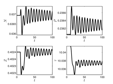
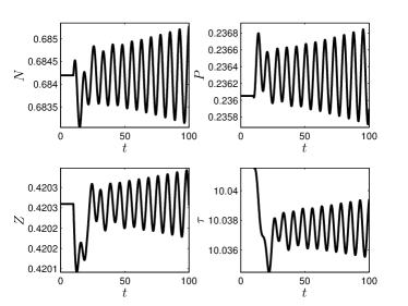
Refer to caption
Refer to caption
Figure 6: The time series of a simulation for R=PP+0.159𝑅𝑃𝑃0.159R=\frac{P}{P+0.159}, δ0=δsubscript𝛿0𝛿\delta_{0}=\delta, m=6𝑚6m=6, and NT=100.49subscript𝑁𝑇superscript100.49N_{T}=10^{0.49} (left) and NT=100.51subscript𝑁𝑇superscript100.51N_{T}=10^{0.51} (right). The initial conditions were chosen near the equilibrium solution. In the case of NT=100.49subscript𝑁𝑇superscript100.49N_{T}=10^{0.49}, the simulation suggests that the equilibrium solution is stable, but in the case of NT=100.51subscript𝑁𝑇superscript100.51N_{T}=10^{0.51}, it suggests that the equilibrium solution is unstable. This agrees with Figure 4 (on the right, second from the top), which indicated that there is a zero eigenvalue at m=6𝑚6m=6 and NT=100.50subscript𝑁𝑇superscript100.50N_{T}=10^{0.50}. Also plotted is the time series of the τ(m,PT)𝜏𝑚subscript𝑃𝑇\tau(m,P_{T}), which is the state-dependent delay

Figure 7 shows a subinterval of the time series of a simulation for l=0.159𝑙0.159l=0.159, δ0=δsubscript𝛿0𝛿\delta_{0}=\delta, m=8𝑚8m=8, and NT=100.73subscript𝑁𝑇superscript100.73N_{T}=10^{0.73}. For these values Figures 2 and 3 together show that there are about five pairs of eigenvalues with real parts close to zero. Thus, we might expect the solution to exhibit up to five frequencies. In Figure 7 we see that the solution is very irregular, which is not surprising given the predicted spectrum shown in Figure 3.
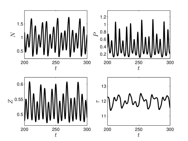
Refer to caption
Figure 7: A subinterval of the time series of a simulation for R=PP+0.159𝑅𝑃𝑃0.159R=\frac{P}{P+0.159}, δ0=δsubscript𝛿0𝛿\delta_{0}=\delta, m=8𝑚8m=8, and NT=100.73subscript𝑁𝑇superscript100.73N_{T}=10^{0.73}. The state-dependent delay, τ(m,Pt)𝜏𝑚subscript𝑃𝑡\tau(m,P_{t}) is also shown. This simulation shows the possibility of very irregular and possibly chaotic solutions to system (15)

10 Discussion

We have looked at a model of a closed planktonic ecosystem that depends on the maturity structure of the immature zooplankton. Using techniques in [19] and [20], we were able to transform the model into a delay differential equation with a state-dependent threshold-type delay or a delay differential equation with a state-independent delay. Such transformations allowed us to use results readily available from the theory of delay differential equations to study the qualitative features of the model, such as existence and uniqueness of solutions, boundedness, persistence, and stability. For instance, we showed that solutions exist for all time, remain positive, and are bounded, which are desirable features for an ecological model to have.

Being able to represent a system in a variety of ways is very beneficial from a mathematical perspective, as we are able to choose the framework that is most convenient for the situation at hand. For instance, the state-independent delay differential equation was useful for applying well-established theory for functional differential equations with fixed delay, as well as performing numerical simulations. The state-dependent threshold differential equation was convenient for computing the linearization and for arguing qualitative results. The partial differential equation was useful since it represents the model in its most intuitive form, and therefore offers the best framework for interpreting results.

Furthermore, in a practical sense, the different models offer flexibility in what initial data is required for numerical simulations. For instance, in some situations it may be convenient to measure the spectrum of the juvenile zooplankton at a given time, while in other situations it may be more convenient to measure the histories of the phytoplankton and mature zooplankton over a sufficiently long time interval. Since it is possible to transform between the PDE and TDE models, the type of data obtained for the initial conditions does not necessarily dictate which equations we need to use to simulate the ecosystem.

A key parameter in the study of closed ecosystems is the amount of biomass, which is fixed by the initial conditions. General results include the existence of two critical values of the total biomass. The first is the minimum amount needed to sustain the phytoplankton population, which we have called NT1subscript𝑁𝑇1N_{T1}. If the biomass is less than NT1subscript𝑁𝑇1N_{T1}, then the phytoplankton and zooplankton both become extinct, as there is not enough biomass to sustain their populations. Conversely, if the biomass is greater than NT1subscript𝑁𝑇1N_{T1}, then the phytoplankton do not become extinct. The second critical value of the total biomass, which we have called NT2subscript𝑁𝑇2N_{T2}, is the minimum amount needed to sustain the zooplankton population. If the total biomass is less than NT2subscript𝑁𝑇2N_{T2} then the zooplankton population becomes extinct, but does not if the biomass is greater than NT2subscript𝑁𝑇2N_{T2}. We have shown that if the total biomass is greater than NT1subscript𝑁𝑇1N_{T1}, but less than NT2subscript𝑁𝑇2N_{T2}, then the system globally approaches a unique, phytoplankton-only equilibrium solution that depends on the total biomass. Future work might include further study of the system when the biomass is greater than NT2subscript𝑁𝑇2N_{T2}, including a formal study of weak/strong (uniform) persistence [3] and possibly global behaviour of solutions. Here, for NT>NT2subscript𝑁𝑇subscript𝑁𝑇2N_{T}>N_{T2}, we mainly focused on local stability of the unique equilibrium solution with numerical techniques for a chosen set of parameter values.

In the case when the juvenile zooplankton have a zero mortality rate, (δ0=0subscript𝛿00\delta_{0}=0), the stability results have a strong dependence on the total biomass (NTsubscript𝑁𝑇N_{T}) while the required level of maturity (m𝑚m) is less significant. In essence, it seems that the time to maturity does not matter if juvenile zooplankton are not being lost due to mortality. However, when we allow them to have a positive mortality rate (δ0>0subscript𝛿00\delta_{0}>0), the required level of maturity becomes more important with regards to stability. In this case, Figure 4 suggests that m𝑚m must increase with NTsubscript𝑁𝑇N_{T} in order to maintain stability of the phytoplankton-zooplankton equilibrium.

As well as stable behaviour, the model ecosystem can simple exhibit periodic solutions as well as more complicated dynamics. We saw complicated orbits in many cases where parameters were such that the characteristic equation had multiple pairs of eigenvalues that had real parts close to zero.

Further work may include adding structure to the immature phytoplankton population in a similar way to what was done for the immature zooplankton. In [13], we have included a delay in nutrient recycling while ignoring the structure of the immature zooplankton, but a more complete model would include both of these effects. It may also be worthwhile to see how non-linear closure terms affect the overall behaviour of the system when the zooplankton size-structure is present. An investigation into the role of this closure term in models without such size-structure is given in [5] and is generally considered to be very significant in determining the dynamics that can occur. Spatial structure can also be added, but similar transformations between partial differential equations and delay differential equations may not be possible in this case.

References

  • [1] S. P. Blythe, R. M. Nisbet, and W. S. C. Gurney. The dynamics of population models with distributed maturation periods. Theor Popul Biol, 25(3):289–311, 1984.
  • [2] G. Bocharov and K. P. Hadeler. Structured population models, conservation laws, and delay equations. J Diff Eqn, 168(1):212–237, 2000.
  • [3] G. Butler, H. I. Freedman, and P. Waltman. Uniformly persistent systems. Proc. Am. Math. Soc., 96:425–430, 1986.
  • [4] K. L. Cooke and W. Huang. On the problem of linearization for state-dependent delay differential equations. Proceedings of the American Mathematical Society, pages 1417–1426, 1996.
  • [5] A. M. Edwards. Adding detritus to a nutrient-phytoplankton-zooplankton model: a dynamical-systems approach. J. Plankton Res., 23(4):389–413, 2001.
  • [6] P. J. S. Franks. NPZ models of plankton dynamics: Their construction, coupling to physics, and application. J. Oceanogr., 58:379–387, 2002.
  • [7] W. C. Gentleman and A. B. Neuheimer. Functional responses and ecosystem dynamics: how clearance rates explain the influence of satiation, food-limitation and acclimation. J. Plankton Res., 30(11):1215–1231, 2008.
  • [8] K. Gopalsamy. Stability and oscillations in delay differential equations of population dynamics. Kluwer Academic, Dordrecht, 1992.
  • [9] W. J. F. Govaerts. Numerical Methods for Bifurcations of Dynamical Equilibria. SIAM, Philadelphia, 2000.
  • [10] W. S. C. Gurney, R. M. Nisbet, and J. H. Lawton. The systematic formulation of tractable single-species models incorporating age structure. Journal of Animal Ecology, 52(2):479–495, 1983.
  • [11] J. K. Hale and S. M. Lunel. Introduction to Functional Differential Equations. Springer-Verlag, New York, 1993.
  • [12] C. S. Holling. The functional response of invertebrate predators to prey density. Mem. Entomol. Soc. Can., (48):1–86, 1966.
  • [13] M. Kloosterman, S. A. Campbell, and F. J. Poulin. A closed NPZ model with delayed nutrient recycling. J. Math. Biol., pages 1–36, 2013.
  • [14] E. McCauley, W. W. Murdoch, and R. M. Nisbet. Growth, reproduction, and mortality of daphnia pulex leydig: life at low food. Funct. Ecol., 4(4):505–514, 1990.
  • [15] J. A. J. Metz and O. Diekmann. The dynamics of physiologically structured populations. Lecture notes in biomathematics, 68, 1986.
  • [16] J. D. Murray. Mathematical biology. Springer-Verlag, Berlin, 1989.
  • [17] R. M. Nisbet and W. S. C. Gurney. The systematic formulation of population models for insects with dynamically varying instar duration. Theoretical Population Biology, 23(1):114–135, 1983.
  • [18] F. J. Poulin and P. J. S. Franks. Size-structured planktonic ecosystems: Constraints, controls and assembly instructions. J. Plankton Res., 32(8):1121–1130, 2010.
  • [19] H. L. Smith. Threshold delay differential equations are equivalent to standard fde’s. In Equadiff, pages 899–904, 1991.
  • [20] H. L. Smith. Reduction of structured population models to threshold-type delay equations and functional differential equations: A case study. Mathematical Biosciences, 113:1–23, 1993.
  • [21] H. L. Smith. A structured population model and a related functional differential equation: Global attractors and uniform persistence. Journal of Dynamics and Differential Equations, 6(1):71–99, 1994.
  • [22] H. L. Smith. Equivalent dynamics for a structured population model and a related functional differential equation. Journal of Mathematics, 25(1), 1995.
  • [23] D. Sulsky, R. R. Vance, and W. I. Newman. Time delays in age-structured populations. Journal of theoretical biology, 141(3):403–422, 1989.
  • [24] H. O. Walther. Differential equations with locally bounded delay. J. Differential Equations, 252:3001–3039S, 2012.
  • [25] P. Waltman and E. Butz. A threshold model of antigen-antibody dynamics. Journal of Theoretical Biology, 65(3):499–512, 1977.
  • [26] J. S. Wroblewski, J. L. Sarmiento, and G. R. Flierl. An ocean basin scale model of plankton dynamics in the North Atlantic 1. solutions for the climatological oceanographic conditions in May. Glob. Biogeochem. Cycles, 2:199–218, 1988.