Fast, adaptive, high order accurate discretization of the Lippmann-Schwinger equation in two dimensions

Abstract

We present a fast direct solver for two dimensional scattering problems, where an incident wave impinges on a penetrable medium with compact support. We represent the scattered field using a volume potential whose kernel is the outgoing Green’s function for the exterior domain. Inserting this representation into the governing partial differential equation, we obtain an integral equation of the Lippmann-Schwinger type. The principal contribution here is the development of an automatically adaptive, high-order accurate discretization based on a quad tree data structure which provides rapid access to arbitrary elements of the discretized system matrix. This permits the straightforward application of state-of-the-art algorithms for constructing compressed versions of the solution operator. These solvers typically require $O(N^{3/2})$ work, where $N$ denotes the number of degrees of freedom. We demonstrate the performance of the method for a variety of problems in both the low and high frequency regimes.

1 Introduction

The problem of acoustic or electromagnetic scattering from penetrable media arises in a variety of applications, from medical imaging to remote sensing, nondestructive testing, sonar, radar and geophysics. In the two-dimensional setting, the governing partial differential equation is the time-harmonic Helmholtz equation

$$\Delta u(x)+\kappa^{2}(1+q(x))u(x)=0,\quad x\in\mathbb{R}^{2}$$ (1)

where $u(x)$ is the total field and $\kappa$ is the background wavenumber, and the perturbation (or contrast function) $q(x)$ has compact support, say in a domain $\Omega$. Note that for $q(x)>-1$ the solution is propagating, while for $q(x)<-1$ it is evanescent. Using the standard language of scattering theory, the total field $u(x)$ can be expressed as the sum of a known incident field $u^{\text{inc}}(x)$ and an unknown scattered field $u^{\text{scat}}(x)$. In order to be well-posed, the latter must satisfy the Sommerfeld radiation condition (2).

$$\lim_{r\to\infty}r^{1/2}\left(\dfrac{\partial u}{\partial r}^{\text{scat}}-i\kappa u^{\text{scat}}\right)=0\,\,\,\,r=|x|$$ (2)

The incoming field is assumed to satisfy the homogeneous equation

$$\Delta u^{\text{inc}}(x)+\kappa^{2}u^{\text{inc}}(x)=0$$ (3)

in some neighborhood $D$ containing $\Omega$. From eqs. (1) and (3), it follows that the unknown scattered field satisfies

$$\Delta u^{\text{scat}}(x)+\kappa^{2}q(x)u^{\text{scat}}=-k^{2}q(x)u^{\text{inc}}(x)\,.$$ (4)

While PDE-based methods can be used to discretize (4) directly (see [22, 24, 45] and the references therein), we choose to represent the scattered field $u^{\text{scat}}$ using a volume potential

$$u^{\text{scat}}(x)=V[\psi](x)=\int_{\Omega}G_{\kappa}(x,y)\psi(y)dy,$$ (5)

where $\psi(y)$ is an unknown density and $G_{\kappa}(x,y)$ is the outgoing free space Green’s function, given by

$$G_{\kappa}(x,y)=\dfrac{i}{4}H_{0}^{(1)}(\kappa|x-y|)\,.$$ (6)

It is well-known that the operator $V$ in eq. (5) is bounded as a map from $L^{2}(\Omega)$ to $H^{2}(D)$ and compact as an operator acting on $L^{2}(\Omega)$ [19]. Further, it is straightforward to see that, substituting the representation (5) into eq. (4), we obtain the Lippmann-Schwinger integral equation

$$\psi(x)+\kappa^{2}q(x)V[\psi](x)=f(x)\,$$ (7)

where $f(x)=-\kappa^{2}q(x)u^{\text{inc}}(x)$. This is an invertible (resonance-free) Fredholm equation of the second kind with a weakly singular kernel.

Remark 1.

The Lippmann-Schwinger equation is often used to denote an alternative formulation [17]:

$$u(x)-\kappa^{2}V[uq](x)=u^{\text{inc}}(x)\,,$$ (8)

derived by convolving the original Helmholtz equation (1) with the governing Green’s function $G_{\kappa}(x,y)$. The equation (7) has two advantages. First, one is often interested in gradients of the scattered field. This can be done from (5), with full precision by quadrature. Using (8), one would need to numerically differentiate the computed solution, with the attendant loss of accuracy. The formulation (7) is also slightly easier to work with, since the contrast function $q(x)$ appears as a (left) diagonal multiplier of the volume integral operator, whereas it appears inside the volume integral in the classical scheme.

The Lippmann-Schwinger equation poses several numerical challenges. First, it leads to a large, dense linear system of equations for $\psi(x)$. Second, it may involve a complicated contrast function $q(x)$, requiring adaptive mesh refinement for effective resolution. Third, it may be ill-conditioned due to multiple scattering once the contrast $q(x)$ and $\kappa$ are large. The literature in this area is substantial, and we do not seek to review it here. Some relevant prior work on volume integral-based methods, fast solvers, and numerical scattering theory includes [3, 4, 5, 6, 8, 9, 10, 11, 12, 13, 14, 15, 16, 18, 21, 23, 24, 26, 27, 30, 28, 29, 31, 33, 34, 36, 37, 38, 39, 42, 43].

Our goal in this paper is to develop a fast, adaptive, high-order accurate, direct solver, which shares features with many of the algorithms in the papers cited above. We concentrate, in particular, on developing a framework that permits the rapid computation of entries in the governing system matrix, once the adaptive data structure has been specified. With this capability in hand, it is straightforward to make use of modern hierarchical direct solvers.

There has been relatively little attention paid to the adaptive discretization issue, and fast direct solvers for volume integral equations are typically implemented on either uniform Cartesian or polar grids. This is a perfectly sensible approach, especially when first developing fast solvers, whether based on separation of variables and FFTs or hierarchical direct methods [2, 11, 12, 15, 21, 24, 43].

In the next section, we describe a high-order adaptive approach to discretization of the unknown density $\psi$ in (7), followed by a detailed explanation of how one can rapidly compute the matrix entries of the fully discretized system. We then discuss a fast solver for the Lippmann-Schwinger equation using the HODLR method of [4, 5] and present numerical examples illustrating the performance of the scheme.

2 Discretization

We assume that we are given a square domain $D$ which contains the support of a known contrast function $q(x)$. By inspection of the Lippmann-Schwinger equation (7), $D$ clearly contains the support of our right-hand side $f(x)=-\kappa^{2}q(x)u^{\text{inc}}(x)$, and therefore the unknown $\psi(x)$ as well. We subdivide $D$ using an adaptive quad-tree, ensuring that $q(x)$ and $f(x)$ are well-resolved, and that the number of points per wavelength is greater than or equal to a user-specified parameter in each leaf node, on which we impose a $p\times p$ grid (based on a uniform grid for $p=4$ and based on a tensor product Chebyshev grid for $p>4$). The unknowns are taken to be the values of $\psi$ at the $p\times p$ grids on every leaf node, and we will seek to enforce the integral equation at the same nodes, corresponding to a Nyström discretization of the integral equation. If we let $\vec{\psi}$ denote the vector of function values at all leaf node grid points and we let $\vec{f}$ denote the vector of right-hand side values at those same leaf node grid points, then the discrete version of eq. (7) takes the form

$$A\vec{\psi}=\vec{f}\,.$$ (9)

2.1 The adaptive data structure

The domain $D$ is decomposed hierarchically, as follows. Grid level 0 is defined to be the domain $D$ itself. Grid level $l+1$ is obtained by recursive subdivision of each box $\mathcal{B}$ at level $l$ into four child boxes (Fig. 1). $\mathcal{B}$ is referred to as their parent. We allow for adaptivity, so that not all boxes at level $l$ are necessarily divided. We will, however, require that the tree satisfy a standard restriction - namely, that two leaf nodes which share a boundary point must be no more than one refinement level apart. Refinement is controlled by the following two criteria. First, given the wavenumber (Helmholtz parameter) $\kappa$, a box is subdivided if it is of side length $L_{\mathcal{B}}$ and $\kappa L_{\mathcal{B}}\geq 2\pi M$, for a user-specified parameter $M$. This ensures that there are at least $M$ points per wavelength in each linear dimension. Second, we ensure that the contrast $q(x)$ and the right hand side $f(x)$ are both well-resolved. For this, suppose we are given a leaf node $\mathcal{B}$ at level $l$. We evaluate the functions $q(x)$ and $f(x)$ at tensor product Chebyshev nodes on $\mathcal{B}$ and compute the coefficients of the corresponding $p$th order Chebyshev approximation, which we will denote by $P_{\mathcal{B}}$. We then subdivide the box into four child boxes $\mathcal{B}_{i}$, and compute $q(x)$ and $f(x)$ at tensor product Chebyshev nodes on each one. If the computed values in the chid boxes agree with $P_{\mathcal{B}}$ to a user-specified tolerance $\epsilon$, we terminate the refinement at box $\mathcal{B}$. Otherwise, we add the children to the data structure at level $l+1$ and continue until the approximation criterion is satisfied.

Fig. 1: Box $\mathcal{B}$ and its four children

The procedure described above will not, in general, produce a level-restricted tree. It is straightforward, however, to add further refinements until that criterion is satisfied as well (Fig. 2).

(a) Adaptive quad tree before level restriction

(b) Adaptive quad tree after level restriction

Fig. 2: An adaptive quad-tree and its level-restricted refinement.

2.2 The volume integral

We shall assume that there are $M$ leaf nodes in the tree, denoted by $\{D_{m}\}$, so that

$$D=\cup_{m=1}^{M}D_{m}\,.$$

Thus, the volume integral defining the scattered field (5) can be written in the form:

$$u^{\text{scat}}(x)=V[\psi](x)=\displaystyle\sum_{m=1}^{M}\dfrac{i}{4}\int_{D_{m}}H_{0}^{(1)}(\kappa|x-y|)\psi(y)dy$$ (10)

Note that, since we are using an adaptive tree, the various $D_{m}$ can be at arbitrary levels in the spatial hierarchy. To obtain a Nyström method, it remains to discuss the computation of a high-order accurate discretization of $V[\psi]$. For this, we will require some notation. We let the values of the unknown density $\psi$ on leaf node $D_{m}$ be given by $\psi_{m,j}\approx\psi(x_{j})$ for $j=1,\dots,p^{2}$ where $x_{j}$ is one of the $p^{2}$ grid points on $D_{m}$ (Fig. 3).

Fig. 3: Discretization points for a leaf node $D_{m}$ and two neighboring boxes at different levels of the hierarchy. A uniform grid is used for 4$th$ order accuracy and a tensor-product Chebyshev mesh for higher order accuracy.

When clear from context, we write the full unknown vector as $\psi_{j}$ for $j=1,\dots,N$ where $N=p^{2}M$ is the total number of unknowns. We write $q_{j}=q(x_{j})$ and $f_{j}=f(x_{j})$ for the contrast function and and the right-hand side, respectively, at the corresponding grid points.

2.2.1 Polynomial approximation

In order to obtain $p^{th}$ order accuracy, we build a $p$th order polynomial approximation to the density $\psi$ on each leaf node $\mathcal{B}$ of length $L_{\mathcal{B}}$ centered at $(\mathcal{B}_{1},\mathcal{B}_{2})$. For this, we let $x=(\xi_{1},\xi_{2})$ and let $b_{j}(\xi_{1},\xi_{2})$ denote a suitable basis for polynomials of two variables of degree $p-1$. That is, the $b_{j}(\xi_{1},\xi_{2})$ should span $\{\xi_{1}^{a}\xi_{2}^{b}:0\leq a+b<p\text{ with }a,b\in\mathbb{N}^{+}\}$. The number of such basis functions is clearly $N_{p}=\dfrac{p(p+1)}{2}$. In practice, we use the simple monomials $\xi_{1}^{a}\xi_{2}^{b}$ for fourth order accuracy and Chebyshev polynomials of the form $T_{a}(\xi_{1})T_{b}(\xi_{2})$ for higher order schemes, scaled to the unit box $[-1/2,1/2]^{2}$.

Suppose now that we are given a $p$th order polynomial defining $\psi(\xi_{1},\xi_{2})$ on $\mathcal{B}$:

$$\psi_{\mathcal{B}}(\xi_{1},\xi_{2})=\displaystyle\sum_{l=1}^{N_{p}}c_{\mathcal{B}}(l)b_{l}\left(\dfrac{\xi_{1}-\mathcal{B}_{1}}{L_{\mathcal{B}}},\dfrac{\xi_{2}-\mathcal{B}_{2}}{L_{\mathcal{B}}}\right)\,.$$ (11)

For the tensor product grid points $x_{i}=(\xi_{i,1},\xi_{i,2})$ lying in $\mathcal{B}$, we define the interpolation matrix $Q:\mathbb{R}^{N_{p}}\rightarrow\mathbb{R}^{p^{2}}$ with entries $Q_{il}$ by

$$Q_{il}=b_{l}\left(\dfrac{\xi_{i,1}-\mathcal{B}_{1}}{L_{\mathcal{B}}},\dfrac{\xi_{i,2}-\mathcal{B}_{2}}{L_{\mathcal{B}}}\right)\,,$$

so that

$$\psi_{\mathcal{B}}(\xi_{i,1},\xi_{i,2})=\displaystyle\sum_{l=1}^{N_{p}}Q_{il}c_{\mathcal{B}}(l)\,.$$

Note that in eq. (11), the basis functions are independent of the level of box $\mathcal{B}$ in the quad tree, since we normalize by the box dimension $L_{\mathcal{B}}$. If we let $\vec{\psi_{\mathcal{B}}}\in\mathbb{R}^{p^{2}}$ denote the function values at the tensor product grid points in standard ordering, and $\vec{c}_{\mathcal{B}}=(c_{\mathcal{B}}(1),c_{\mathcal{B}}(1),\dots,c_{\mathcal{B}}(N_{p}))\in\mathbb{R}^{N_{p}}$, then $\vec{\psi_{\mathcal{B}}}\approx Q\vec{c_{\mathcal{B}}}$. Let us denote by $Q^{\dagger}$ the pseudoinverse of $Q$, so that the coefficients $\vec{c_{\mathcal{B}}}$ can be computed from $\vec{\psi_{\mathcal{B}}}$ via

$$\vec{c_{\mathcal{B}}}=Q^{\dagger}\vec{\psi_{\mathcal{B}}}\,.$$

The cost of computing $Q^{\dagger}$ by means of the singular value decomposition is negligible. Moreover, this is done only once and the pseudoinverse is stored.

Suppose now that we wish to compute an arbitrary matrix entry $V_{ij}$ corresponding to a $p$th order accurate Nyström discretization of $V[\psi]$ in (10). We assume that $x_{j}$ lies in box $\mathcal{B}$ and that $x_{i}$ is an arbitrary point in the adaptive quad tree data structure (including possible $\mathcal{B}$ itself). Then, for $p$th order accuracy, the contribution of the $j$th grid point to the $i$th target point is precisely

$$V_{ij}\equiv\dfrac{i}{4}\sum_{l=1}^{N_{p}}Q^{\dagger}_{lj}\int_{\mathcal{B}}H_{0}^{(1)}(\kappa|x_{i}-y|)b_{l}\left(\dfrac{y_{1}-\mathcal{B}_{1}}{L_{\mathcal{B}}},\dfrac{y_{2}-\mathcal{B}_{2}}{L_{\mathcal{B}}}\right)\,dy_{1}dy_{2}\,,$$ (12)

where $y=(y_{1},y_{2})$. This follows from the fact that the $i$th column of $Q^{\dagger}$ is a vector in $\mathbb{R}^{N_{p}}$, consisting of the contributions (or projections) of the $i$th grid point onto each of the $N_{p}$ basis functions. Thus, the $(i,j)$ entry of the full matrix in the linear system in eq. (9) is given by

$$A_{ij}=\delta_{ij}+\kappa^{2}q(x_{i})V_{ij}\,.$$ (13)

It is worth emphasizing that the amount of work in computing $V_{ij}$ (or $A_{ij}$) is independent of $N$ (the total number of discretization points). Each entry could, for example, be computed by adaptive quadrature on the fly. We wish, however, to be able to evaluate an arbitrary matrix entry in only a few floating point operations. The remainder of this section is devoted to an extremely efficient method for this task, based on the geometric relations between $x_{i}$ and $x_{j}$.

Definition 1.

The colleagues of a box $\mathcal{B}$ are boxes at the same level in the tree hierarchy which share a boundary point with $\mathcal{B}$. ($\mathcal{B}$ is considered to be a colleague of itself.) Note that each box has at most $9$ colleagues (Fig. 4).

Fig. 4: Colleagues

The coarse neighbors of $\mathcal{B}$ are leaf nodes that are one level higher than that of $\mathcal{B}$ and which share a boundary point with $\mathcal{B}$. Note that there can be at most $12$ coarse neighbors (Fig. 5).

Fig. 5: Coarse neighbors

The fine neighbors of $\mathcal{B}$ are leaf nodes that are one level below that of $\mathcal{B}$ and share a boundary point with $\mathcal{B}$. Note that there can be at most $12$ fine neighbors (Fig. 6).

Fig. 6: Fine neighbors

The separated fine neighbors of $\mathcal{B}$ are non-neighboring leaf nodes that are one level below that of $\mathcal{B}$ and whose parent shares a boundary point with $\mathcal{B}$. There are at most $16$ separated fine neighbors (Fig. 7).

Fig. 7: Separated fine neighbors

All other leaf nodes are separated from $\mathcal{B}$ by at least the length $L_{\mathcal{B}}$ and are considered its far field.

2.3 Far-field interactions

The easiest case to consider is when $x_{i}$ lies in the far field of box $\mathcal{B}$. If we let $x_{i}=(\xi_{i,1},\xi_{i,2})$ and denote by $\theta_{i}$ the polar angle of $x_{i}$ with respect to the box center $(\mathcal{B}_{1},\mathcal{B}_{2})$, the Graf addition theorem [1, 40] states that

$$H_{0}^{(1)}(\kappa|x_{i}-y|)=\displaystyle\sum_{n=-\infty}^{\infty}H_{n}(\kappa\|(\xi_{i,1}-\mathcal{B}_{1},\xi_{i,2}-\mathcal{B}_{2})\|)J_{n}(\kappa\|(y_{1}-\mathcal{B}_{1},y_{2}-\mathcal{B}_{2})\|)e^{in(\theta_{i}-\theta_{y})}$$ (14)

where $\theta_{y}$ denotes the polar angle of the point $y\in\mathcal{B}$ with respect to the box center. Since the dimensions of the leaf node are assumed to satisfy $\kappa L_{\mathcal{B}}\leq 8$, we can truncate eq. (14) after about $L+8$ terms with an error of approximately $2^{-L}$. It is easy to verify that

$$V_{ij}\approx\frac{i}{4}\sum_{n=-L}^{L}M_{n}(j)H_{n}(\kappa\||x_{i}-(\mathcal{B}_{1},\mathcal{B}_{2})\|)e^{il\theta_{i}}$$ (15)

where

$$M_{n}(j)=\sum_{l=1}^{N_{p}}C_{nl}Q^{\dagger}_{lj}$$ (16)

and

$$C_{nl}=\displaystyle\int_{\mathcal{B}}J_{n}(\kappa\|(y_{1}-\mathcal{B}_{1},y_{2}-\mathcal{B}_{2})\|)e^{-il\theta_{y}}b_{l}\left(\dfrac{y_{1}-\mathcal{B}_{1}}{L_{\mathcal{B}}},\dfrac{y_{2}-\mathcal{B}_{2}}{L_{\mathcal{B}}}\right)dy_{1}dy_{2}\,.$$ (17)

Note that the integrals in (17) are smooth and need to be computed only once per level at negligible cost. Moreover, $M_{n}(j)$ also only needs to be computed once per level. Thus, the cost of computing a far field matrix entry to fourteen digits of accuracy is essentially that of evaluating the multipole expansion (15) with $L=45$, which can be done about one million times per second on a single core.

2.4 Separated fine neighbors

The multipole expansion for $\mathcal{B}$ in the previous section is slowly converging for the separated fine neighbors (Fig. 7). However, it is straightforward to create four child boxes from $\mathcal{B}$ and to compute the multipole expansions for each of the four children from each basis function $b_{l}\left(\dfrac{y_{1}-\mathcal{B}_{1}}{L_{\mathcal{B}}},\dfrac{y_{2}-\mathcal{B}_{2}}{L_{\mathcal{B}}}\right)$. Evaluating the corresponding multipole expansions at each separated fine neighbor target point yields the desired value $V_{ij}$.

2.5 Near field interactions

For points in the near field, we rewrite (12) in the form:

$$V_{ij}\equiv\sum_{l=1}^{N_{p}}Q^{\dagger}_{lj}V^{\kappa}_{il}\,,$$ (18)

where

$$V^{\kappa}_{il}=\dfrac{i}{4}\displaystyle\int_{\mathcal{B}}H_{0}^{(1)}(\kappa|x_{i}-(y_{1},y_{2})|)b_{l}\left(\dfrac{y_{1}-\mathcal{B}_{1}}{L_{\mathcal{B}}},\dfrac{y_{2}-\mathcal{B}_{2}}{L_{\mathcal{B}}}\right)dy_{1}dy_{2}\,.$$ (19)

It will be convenient to rescale variables so that integrals are always carried out over the unit box. Thus, instead of (19), we write

$$V^{\kappa}_{il}=\dfrac{iL_{\mathcal{B}}^{2}}{4}\displaystyle\int_{U}H_{0}^{(1)}(\kappa L_{\mathcal{B}}r_{i})b_{l}\left(y_{1},y_{2}\right)dy_{1}dy_{2}$$ (20)

where $U=[-0.5,0.5]^{2}$ and $r_{i}=|x_{i}/L_{\mathcal{B}}-(y_{1},y_{2})|$. Note that, in this representation, the integral $V^{\kappa}_{il}$ depends only on the relative coordinates of the target point $x_{i}$ to the unit box $U$. There are only finitely many such possibilities, corresponding to the various target locations in the colleagues, coarse neighbors, or fine neighbors. Thus, the number of such interactions is fixed. $x_{i}$ must be one of $p^{2}$ possible locations in each of $9$ possible colleagues, $12$ possible fine neighbors and $12$ possible coarse neighbors. Thus, we seek to compute tables of dimension $p^{2}\times 9\times p^{2}$, $p^{2}\times 12\times p^{2}$, and $p^{2}\times 12\times p^{2}$, respectively. For this, we use the fact [1, 40] that

$$H_{0}^{(1)}(z)=J_{0}(z)+iY_{0}(z)$$

with

$$J_{0}(z)=\sum_{m=0}^{\infty}\frac{(-1)^{m}}{(m!)^{2}}\left(\frac{z}{2}\right)^{2m},$$

$$Y_{0}(z)=\frac{2}{\pi}\left(\ln\left(\frac{z}{2}\right)+\gamma\right)J_{0}(z)+\frac{2}{\pi}\left(\frac{\frac{1}{4}z^{2}}{(1!)^{2}}-(1+\frac{1}{2})\frac{(\frac{1}{4}z^{2})^{2}}{(2!)^{2}}+(1+\frac{1}{2}+\frac{1}{3})\frac{(\frac{1}{4}z^{2})^{3}}{(3!)^{2}}-\dots\right),$$

where $\gamma$ is Euler’s constant. This permits us to write

$$H_{0}^{(1)}(\kappa L_{\mathcal{B}}r)=\displaystyle\sum_{p=0}^{\infty}c_{p}(\kappa L_{\mathcal{B}})\left(\dfrac{r}{2}\right)^{2p}+\displaystyle\sum_{p=0}^{\infty}d_{p}(\kappa L_{\mathcal{B}})\left(\dfrac{r}{2}\right)^{2p}\log\left(\dfrac{r}{2}\right)$$ (21)

where

$$c_{p}(z)=a_{p}(z)+\dfrac{2i}{\pi}g_{p}(z),\ d_{p}(z)=\dfrac{2i}{\pi}a_{p}(z),\ a_{p}(z)=\dfrac{(-z^{2})^{p}}{(p!)^{2}},\ g_{p}(z)=\left(\gamma+\log(z)-H_{p}\right)a_{p}(\kappa L_{\mathcal{B}}).$$

Here, $H_{0}=0,H_{1}=1,H_{2}=(1+\dfrac{1}{2}),H_{3}=(1+\dfrac{1}{2}+\dfrac{1}{3})$, etc. This permits us to write

$$V^{\kappa}_{il} =\dfrac{iL_{\mathcal{B}}^{2}}{4}\displaystyle\sum_{p=0}^{p_{\max}}c_{p}(\kappa L_{\mathcal{B}})\displaystyle\int_{U}\left(\dfrac{r}{2}\right)^{2p}b_{l}\left(y_{1},y_{2}\right)dy_{1}dy_{2}$$

$$+\dfrac{iL_{\mathcal{B}}^{2}}{4}\displaystyle\sum_{p=0}^{p_{\max}}d_{p}(\kappa L_{\mathcal{B}})\displaystyle\int_{U}\left(\dfrac{r}{2}\right)^{2p}\log\left(\dfrac{r}{2}\right)b_{l}\left(y_{1},y_{2}\right)dy_{1}dy_{2}\,,$$ (22)

for a suitable choice of $p_{max}$.

The integrals over $U$ in eq. (22) are independent of the wavenumber $\kappa$, so we may tabulate these values to double precision accuracy using adaptive Gaussian quadrature. For $\kappa L_{\mathcal{B}}\leq 8$, it is easy to verify that $p_{max}=60$ is sufficient to obtain fourteen digits of accuracy. The quantities $V^{\kappa}_{il}$ are then obtained using $O(p_{max})$ floating point operations. The storage requirements for this scheme are:

$p^{2}\times N_{p}\times 9\times(2p_{\max}+2)$	for colleagues
$p^{2}\times N_{p}\times 12\times(2p_{\max}+2)$	for fine neighbors
$p^{2}\times N_{p}\times 12\times(2p_{\max}+2)$	for coarse neighbors.

Unfortunately, for $\kappa L_{\mathcal{B}}>4$, the computation in (22) can be subject to catastrophic cancellation. (The series oscillates in sign and involves intermediate terms of large magnitude.) This loss of precision is easily overcome by subdividing $\mathcal{B}$ into four children and generating tables for each child box. With this scheme, the storage costs remain negligible and the matrix entries $V_{ij}$ corresponding to local interactions are computed using only a few hundred floating point operations.

3 Fast direct solvers

The reason we have focused in this paper on the rapid computation of matrix entries is that a new generation of fast solvers has been developed over the last decade or so which permits the inversion of equations such as the Lippmann-Schwinger equation in $O(N^{3/2})$ work. All that is required is a suitable ordering of the unknowns and access to matrix entries on the fly. For the sake of simplicity, we have chosen to use the HODLR scheme of [4, 5]. This solver relies on a hierarchical partitioning of the matrix into a sequence of off-diagonal low-rank blocks (from which the acronym is derived). More precisely, the off-diagonal blocks are approximated using low-rank factorizations to a user-specified precision $\epsilon$. We refer the reader to the original papers for details and to [6, 8, 9, 13, 14, 15, 18, 30, 28, 25, 26, 27, 33, 35, 39, 41, 46] for related schemes. All of these fast solvers, of course, require sampling at most $O(N^{3/2})$ matrix entries. For PDE-based analogues, see [24, 37, 29] and the references therein.

Several of the methods above have smaller constants than HODLR for volume integral equations with singular kernels, but require a slightly more complicated interface. In fact, in the low frequency regime, some of the methods above require only $O(N\log N)$ work (see, for example, [18, 29]). We postpone such accelerations to a later date.

4 Numerical results

In this section, we illustrate the performance of our adaptive solver for the Lippmann-Schwinger equation. In each example, we use an incoming plane wave propagating in the $x$-direction of the form $u^{\text{inc}}=e^{ikx}$ and calculate the value of the scattered field $u^{\text{scat}}$ on a square $D$ which contains the support of the contrast function $q(x)$.

We will make use of both uniform and adaptive grids. As indicated in section 2, in the adaptive case, we refine the domain $D$ using a quad-tree, halting refinement of a leaf node when it is determined to have resolved the contrast function $q(x)$ and the right-hand side $f(x)$ to a user-specified tolerance $\epsilon$. In order to be conservative, we then use a tolerance of $\epsilon\times 10^{-4}$ in the HODLR solver. The number of terms used in various far field expansions is chosen as in [20]. All simulations in this paper were carried out using a single core of a 2.5GHz Xeon processor.

Example 4.1.

Radially symmetric contrast functions

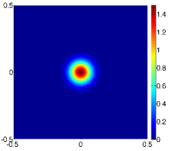
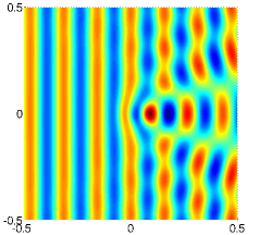
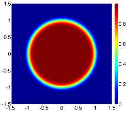
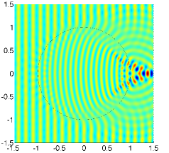
In our first two examples, we consider a radially symmetric contrast function $q(x)$, from which it is straightforward to compute the exact solution using separation of variables, the fast Fourier transform, and a high-order accurate ODE solver (see, for example, [24]). Setting the wavenumber $\kappa=40$, we will use either a Gaussian with $q(x)=1.5e^{-160|x|^{2}}$ or a “flat bump” with $q(x)=0.5\text{erfc}(5(|x|^{2}-1))$, where erfc is the complementary error function [1, 40]

$$\text{erfc}(x)=\frac{2}{\sqrt{\pi}}\int_{x}^{\infty}e^{-t^{2}}~{}dt.$$

In Fig. 8(a) we plot the Gaussian contrast, and in Fig. 8(b) we plot the real part of the total field after solving the scattering problem. In Fig. 9(a) we plot contours of the “flat bump” contrast function, in Fig. 9(b) we plot the real part of the total field, in Fig. 9(c) we show the the adaptive discretization of the domain $D$, and in Fig. 9(d) we plot the contrast function $q(x)$.

(a) Contrast function

(b) Real part of total field

Fig. 8: Gaussian contrast

(a) Contrast function

(b) Real part of total field

(c) Grid for adaptive solver

(d) Surface plot of contrast function

Fig. 9: “Flat bump” contrast

We let $\tilde{u}$ denote the total field calculated using our solver, we let $u$ denote the total field computed using separation of variables as in [24]. Table 1 shows the performance of the solver on a uniform grid.

Table 1: Convergence behavior of Lippmann-Schwinger solver on uniform grid for Gaussian contrast. $N$ denotes the number of discretization points, $e(x)=|u(x)-\tilde{u}(x)|$ is the error at the point $x$. $(0.5,0)$ is well inside the support of the contrast function and $(1,0.5)$ is a point where $q(x)$ has vanished to machine precision. $Time$ is the time required by the fast solver.

$N$	$e(0.5,0)$	$e(1,0.5)$	Time
$256$	$0.8925E+0$	$0.4890E+0$	$0.14$
$1024$	$0.1809E+0$	$0.1406E+0$	$1.16$
$4096$	$1.0938E-2$	$9.6485E-3$	$12.93$
$16384$	$3.1169E-4$	$3.2633E-4$	$104.1$
$65536$	$1.4300E-5$	$1.2537E-5$	$844.8$
$262144$	$8.8874E-7$	$6.4485E-7$	$6869.7$

It is straightforward to check from Table 1 that the convergence rate is approximately fourth order (for a target either within the support of $q(x)$ or in its exterior). The CPU requirements of the solver can also be seen to scale approximately as $O(N^{3/2})$.

We now solve both the Gaussian and flat bump problems using our adaptive refinement strategy. Tables 2 and 3 summarize the corresponding numerical results.

Table 2: Performance of adaptive solver for Gaussian contrast. $\epsilon$ is the tolerance requested from adaptive discretization of the data. The other columns are the same as in Table 1.

$\epsilon$	$N$	$e(0.5,0)$	$e(1,0.5)$	Time
$1E-4$	$4096$	$1.09E-2$	$9.65E-3$	$12.3$
$1E-5$	$4864$	$7.89E-4$	$1.20E-4$	$16.2$
$1E-6$	$6400$	$2.99E-4$	$3.33E-4$	$30.4$
$1E-7$	$10240$	$4.83E-5$	$8.75E-6$	$78.7$
$1E-8$	$16384$	$1.13E-5$	$5.35E-6$	$190.1$
$1E-9$	$34816$	$2.30E-6$	$3.86E-7$	$650.6$
$1E-10$	$70912$	$7.14E-7$	$3.16E-7$	$2350.7$
$1E-11$	$138688$	$4.25E-8$	$1.94E-8$	$7363.4$

Table 3: Performance of adaptive solver for flat bump contrast. $\epsilon$ is the tolerance requested from adaptive discretization of the data and $N$ is the total number of discretization points. $e(x)$ is the error at the point $x$. $(0.5,2)$ is well inside the support of the contrast function and $(3,0.5)$ is a point where $q(x)$ has vanished to machine precision.

$\epsilon$	$N$	$e(0.5,2)$	$e(3,0.5)$	Time
$1E-3$	$10240$	$1.88E-1$	$9.29E-1$	$61.8$
$1E-4$	$40192$	$1.07E-2$	$2.27E-2$	$609.2$
$1E-5$	$134656$	$8.47E-4$	$8.44E-4$	$5561.7$
$1E-7$	$596224$	$2.07E-5$	$1.31E-5$	$75861.5$

As expected, the adaptive method provides significant advantages: for the same accuracy, the problem with a Gaussian contrast function is about ten times faster.

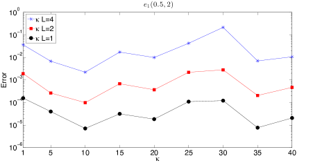
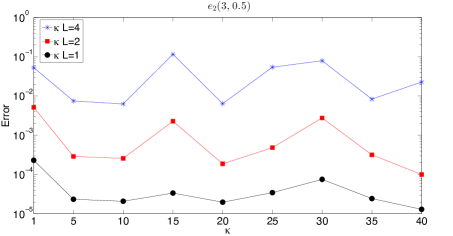
One of the advantages of using the Lippmann-Schwinger formulation over direct discretization of the Helmholtz equation is that Green’s function based methods are not subject to the same kind of grid dispersion error. To verify this, in Figs. 10(a) and 10(b), we plot the error for the flat bump contrast function as a function of wavenumber $\kappa$ at the points $(0.5,2)$ and $(3,0.5)$, respectively. Each curve represents the error for a fixed value of the parameter $\kappa L_{\mathcal{B}}$ on leaf nodes. $\kappa L_{\mathcal{B}}=4,2,1$ correspond to approximately 6, 12 and 24 points per wavelength. Note that the error does not grow with $\kappa$ as it would with a fourth order discretization of the PDE.

(a) Error at the point (0.5,2) as a function of $\kappa$.

(b) Error at the point (3,0.5) as a function of $\kappa$.

Fig. 10: Error as a function of $\kappa$, which determines the size of the domain in wavelengths. The values $\kappa L_{\mathcal{B}}=4,2,1$ correspond to using approximately 6, 12 or 24 points per wavelength.

Example 4.2.

Multiple scattering from well-separated Gaussian bumps

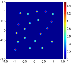
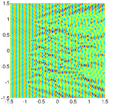
To illustrate the performance of the scheme on a more complicated example, we assume the contrast consists of the sum of $20$ Gaussian bumps of the form

$$q_{j}(x)=1.5e^{-|x-x_{j}|^{2}/a},$$

where the centers $\{x_{j}\}$ are randomly located in $[-1.5,1.5]^{2}$ and $a=0.0013$. With wavenumber $\kappa=60$, the domain is approximately $30$ wavelengths in each linear dimension. We discretize the domain using at least $9$ points per wavelength and resolve the contrast with tolerance $\epsilon$. In Fig. 11(a), we plot the contrast function, and in Fig. 11(b) we plot the real part of the total field calculated using $N=895264$ discretization points with about five digits of accuracy. Fig. 11(c) shows the adaptive grid (at a coarser discretization) and Fig. 11(d) presents a surface plot of the contrast function. Table 4 summarizes our numerical results.

Table 4: Convergence behavior of scattering from multiple Gaussian bumps. $\epsilon$ is the tolerance requested from adaptive discretization of the data and $N$ is the number of discretization points. $\Re(u(x))$ and $\Im(u(x))$ denote the real and imaginary parts of the solution at the point $x$.

$\epsilon$	$N$	$\Re(u(0.5,2))$	$\Im(u(0.5,2))$	$\Re(u(3,0.5))$	$\Im(u(3,0.5))$
$1E-7$	$155056$	$-1.74310E-1$	$-2.89411E-1$	$-7.73067E-1$	$-4.49033E-1$
$1E-8$	$272128$	$-1.74256E-1$	$-2.89433E-1$	$-7.73039E-1$	$-4.49080E-1$
$1E-9$	$441520$	$-1.74268E-1$	$-2.89425E-1$	$-7.73045E-1$	$-4.49084E-1$
$1E-10$	$895264$	$-1.74266E-1$	$-2.89425E-1$	$-7.73044E-1$	$-4.49085E-1$

(a) Contrast function for twenty Gaussian bumps

(b) Real part of total field

(c) Discretization of contrast function

(d) Surface plot of contrast function

Fig. 11: Multiple scattering from 20 Gaussian bumps

Example 4.3.

An example from plasma physics

Radio frequency waves play an important role in magnetic confinement fusion for both heating and diagnostic applications. Radio frequency wave propagation in a fusion reactor can be described using a cold plasma model [7, 32, 44], where the plasma is considered a fluid, possibly involving several species, subject to electric and magnetic forces. Here we consider only electrons, neglecting ions because of the mass ratio. Coupling Newton’s law for the fluid motion with Maxwell’s equations, driven by a current proportional to the electrons velocity, leads to various propagation modes. These are classified by their orientation with respect to the confining magnetic field $\mathbf{B}_{0}$. The ordinary (O) mode corresponds to an electric field parallel to $\mathbf{B}_{0}$, propagating in a plane orthogonal to $\mathbf{B}_{0}$. This particular mode is used for reflectometry, a non-invasive method to probe the plasma density.

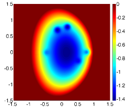
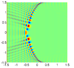
The O mode propagation in the cold plasma model reduces to the Helmholtz equation (1), where the contrast $q(x)$ is proportional to the additive inverse of the electron density, which is compactly supported as the plasma is surrounded by vacuum. Reflectometry relies on the fact that the incoming wave impinging on the plasma can only propagate if the density is smaller than a threshold, called the “cut-off”. In equation (1), the cut-off is implicitly defined by $q(x)=-1$. When the wave reaches the cut-off it cannot propagate further and is reflected back from the plasma. In other words, the plasma forms an evanescent medium when the density is higher than the cut-off density, i.e. where $q(x)<-1$.

In Fig. 12(a), we plot the contrast for an idealized density profile, defined by

$$q(x,y)=\left\{\begin{array}[]{ll}0,&\mbox{if }\psi(x,y)\leq 0.05,\\ -1.5(\psi(x,y)-0.05)-g(x,y)\cos(0.9y),&\mbox{if }\psi(x,y)>0.05,\end{array}\right.$$

where

$$\psi(x,y) =1-(x-0.15(1-x^{2}))^{2}-C(1+0.3x)^{2}y^{2},$$

$$g(x,y) =\sum_{j=1}^{5}a_{j}\exp\left(-\frac{(x-x_{j})^{2}+(y-y_{j})^{2}}{0.01}\right),$$

with $C=0.4987$, and the values of $a_{j}$, $x_{j}$, and $y_{j}$, for $j=1,\ldots,5$, are given in Table 5. We set the wavenumber $\kappa=85$. To solve this problem, we used $N=1060864$ points corresponding to approximately $25$ points per wavelength. The total field calculated by our solver is shown in Figure 12(b). As expected, there is no propagation through the evanescent zone and the incident wave is reflected back at the cut-off. Convergence analysis using Richardson extrapolation indicates that we obtained more than 6 digits of accuracy.

Table 5: Parameters $a_{j}$, $x_{j}$, and $y_{j}$ for the contrast function used in the plasma physics example.

$j$	$a_{j}$	$x_{j}$	$y_{j}$
$1$	$0.45$	$0.80$	$0.00$
$2$	$0.195$	$0.54$	$-0.28$
$3$	$0.51$	$-0.14$	$0.70$
$4$	$0.195$	$-0.50$	$-0.01$
$5$	$0.63$	$0.18$	$0.80$

(a) Contrast function $q(x)$

(b) Real part of total field

Fig. 12: RF wave impinging on plasma.

5 Conclusion

We have presented a high-order method for the Lippmann-Schwinger equation that is of particular value when coupled with modern fast, direct solvers. More precisely, we have developed algorithms for rapidly accessing arbitrary elements of the system matrix consistent with an adaptive Nyström discretization. Our approach extends naturally to three dimensions and to other governing Green’s functions, although some of the accelerations have been developed specifically for the Helmholtz equation and will require modification in other settings.

Our numerical examples were computed using a fourth order accurate approach, but the extension to arbitrary order is straightforward. We are currently working on the coupling of our tools with fast solvers that are quad-tree or oct-tree based, rather than k-d tree-based as in our HODLR solver. These were discussed very briefly in section 3. This will substantially reduce the constant implicit in the $O(N^{3/2})$ notation. We are also working on fast discretization of the Lippmann-Schwinger equation in three dimensions for both acoustic and electromagnetic applications.

References

- [1] M. Abramowitz and I. Stegun, Handbook of Mathematical Functions with Formulas, Graphs, and Mathematical Tables, U.S. Government Printing Office, 1964.
- [2] J. Aguilar and Y. Chen, High-order corrected trapezoidal quadrature ruless for functions with a logarithmic singularity in 2-d, Computers & Mathematics with Applications, 44 (2002), pp. 1031–1039.
- [3] M. B. Amar and F. C. Farnoux, Numerical solution of the lippmann-schwinger equations in photoemission: application to xenon, Journal of Physics B: Atomic and Molecular Physics, 16 (1983), p. 2339.
- [4] S. Ambikasaran and E. Darve, An fast direct solver for partial hierarchically semi-separable matrices — with application to radial basis function interpolation., J. Sci. Comput., (2013), pp. 477–501.
- [5] A. Aminfar, S. Ambikasaran, and E. Darve, A fast block low-rank dense solver with applications to finite-element matrices, arXiv preprint arXiv:1403.5337 [cs-NA], (2014).
- [6] M. Bebendorf, Hierarchical LU decomposition-based preconditioners for BEM, Computing, 74 (2005), pp. 225–247.
- [7] P. T. Bonoli, Electromagneti mode conversion: understanding waves that suddenly change thier nature, Journal of Physics: Conference Series, 16 (2005), pp. 35–39.
- [8] S. Börm, L. Grasedyck, and W. Hackbusch, Hierarchical matrices, Lecture notes, 21 (2003).
- [9] , Introduction to hierarchical matrices with applications, Engineering Analysis with Boundary Elements, 27 (2003), pp. 405–422.
- [10] O. P. Bruno, Wave scattering by inhomogeneous media: efficient algorithms and applications, Physica B: Condensed Matter, 338 (2003), pp. 67 – 73. Proceedings of the Sixth International Conference on Electrical Transport and Optical Properties of Inhomogeneous Media.
- [11] O. P. Bruno and E. Hyde, An efficient, preconditioned, high-order solver for scattering by two-dimensional inhomogeneous media, Journal of Computational Physics, 200 (2004), pp. 670 – 694.
- [12] O. P. Bruno and E. M. Hyde, Higher-order fourier approximation in scattering by two-dimensional, inhomogeneous media., SIAM J. Numerical Analysis, 42 (2005), pp. 2298–2319.
- [13] S. Chandrasekaran, P. Dewilde, M. Gu, W. Lyons, and T. Pals, A fast solver for HSS representations via sparse matrices, SIAM Journal on Matrix Analysis and Applications, 29 (2006), pp. 67–81.
- [14] S. Chandrasekaran, M. Gu, and T. Pals, A fast ULV decomposition solver for hierarchically semiseparable representations, SIAM Journal on Matrix Analysis and Applications, 28 (2006), pp. 603–622.
- [15] Y. Chen, A fast, direct algorithm for the lippmann–schwinger integral equation in two dimensions, Advances in Computational Mathematics, 16 (2002), pp. 175–190.
- [16] H. Cheng, J. Huang, and T. J. Leiterman, An adaptive fast solver for the modified helmholtz equation in two dimensions, Journal of Computational Physics, 211 (2006), pp. 616–637.
- [17] D. Colton and R. Kress, Inverse Acoustic and Electromagnetic Scattering Theory, Springer, 2 ed., 1998.
- [18] E. Corona, P.-G. Martinsson, and D. Zorin, An o (n) direct solver for integral equations on the plane, Applied and Computational Harmonic Analysis, (2014).
- [19] M. Costabel, On the spectrum of volume integral operators in acoustic scattering, in Integral Methods in Science and Engineering, Birkhaüser, Chapter 11, 2015.
- [20] W. Crutchfield, Z. Gimbutas, L. Greengard, J. Huang, V. Rokhlin, N. Yarvin, and J. Zhao, Remarks on the implementation of wideband fmm for the helmholtz equation in two dimensions, Contemporary Mathematics, 408 (2006), pp. 99–110.
- [21] R. Duan and V. Rokhlin, High order quadratures for the solution of scattering problems in two dimensions, Journal of Computational Physics, 228 (2009), pp. 2152–2174.
- [22] B. Engquist and L. Ying, Sweeping preconditioner for the helmholtz equation: hierarchical matrix representation, Communications on Pure and Applied Mathematics, 64 (2011), pp. 697–735.
- [23] F. Ethridge and L. Greengard, A new fast-multipole accelerated Poisson solver in two dimensions, SIAM Journal on Scientific Computing, 23 (2001), pp. 741–760.
- [24] A. Gillman, A. H. Barnett, and P.-G. Martinsson, A spectrally accurate direct solution technique for frequency-domain scattering problems with variable media, BIT Numerical Mathematics, 55 (2015), pp. 141–170.
- [25] S. Goreinov, E. Tyrtyshnikov, and N. Zamarashkin, A theory of pseudoskeleton approximations, Linear Algebra and its Applications, 261 (1997), pp. 1–21.
- [26] L. Greengard, D. Gueyffier, P.-G. Martinsson, and V. Rokhlin, Fast direct solvers for integral equations in complex three-dimensional domains, Acta Numerica, 18 (2009), pp. 243–275.
- [27] W. Hackbusch, L. Grasedyck, and S. Börm, An introduction to hierarchical matrices, Max-Planck-Inst. für Mathematik in den Naturwiss., 2001.
- [28] K. Ho and L. Ying, Hierarchical interpolative factorization for elliptic operators: differential equations, Communications in Pure and Applied Mathematics, (to appear).
- [29] , Hierarchical interpolative factorization for elliptic operators: integral equations, Communications in Pure and Applied Mathematics, (to appear).
- [30] K. L. Ho and L. Greengard, A fast direct solver for structured linear systems by recursive skeletonization, SIAM Journal on Scientific Computing, 34 (2012), pp. 2507–2532.
- [31] T. Hohage, Fast numerical solution of the electromagnetic medium scattering problem and applications to the inverse problem, Journal of Computational Physics, 214 (2006), pp. 224–238.
- [32] L.-M. Imbert-Gerard, Well-posedness of 2d mode conversion model and generalized plaen wave simulations, Journal of Physics: Conference Series, (preprint).
- [33] W. Y. Kong, J. Bremer, and V. Rokhlin, An adaptive fast direct solver for boundary integral equations in two dimensions, Applied and Computational Harmonic Analysis, 31 (2011), pp. 346–369.
- [34] F. Lanzara, V. G. Maz´ya, and G. Schmidt, Numerical solution of the lippmann-schwinger equation by approximate approximations, Journal of Fourier Analysis and Applications, 10 (2004), pp. 645–660.
- [35] E. Liberty, F. Woolfe, P.-G. Martinsson, V. Rokhlin, and M. Tygert, Randomized algorithms for the low-rank approximation of matrices, Proceedings of the National Academy of Sciences, 104 (2007), p. 20167.
- [36] D. Malhotra, A. Gholami, and G. Biros, A volume integral equation stokes solver for problems with variable coefficients, in International Conference for High Performance Computing, Networking, Storage and Analysis, SC14, IEEE, Nov. 2014, pp. 92–102.
- [37] P.-G. Martinsson, A fast direct solver for a class of elliptic partial differential equations, Journal of Scientific Computing, 38 (2009), pp. 316–330.
- [38] , A direct solver for variable coefficient elliptic pdes discretized via a composite spectral collocation method, Journal of Computational Physics, 242 (2013), pp. 460–479.
- [39] P.-G. Martinsson and V. Rokhlin, A fast direct solver for boundary integral equations in two dimensions, Journal of Computational Physics, 205 (2005), pp. 1–23.
- [40] F. W. J. Olver, D. W. Lozier, R. F. Boisvert, and e. C. W. Clark, NIST Handbook of Mathematical Functions, Cambridge University Press, New York, 2010.
- [41] S. Rjasanow, Adaptive cross approximation of dense matrices, in Int. Association Boundary Element Methods Conf., IABEM, 2002, pp. 28–30.
- [42] K. Sandfort, The factorization method for inverse scattering from periodic inhomogeneous media, KIT Scientific Publishing, Karlsruhe, 2010.
- [43] G. Vainikko, Fast solvers of the lippmann-schwinger equation, in Direct and inverse problems of mathematical physics, Springer, 2000, pp. 423–440.
- [44] H. Weitzner, Lower hybrid waves in the cold plasma model, Communications on Pure and Applied Mathematics, 38 (1985), pp. 919–932.
- [45] L. Zepeda-Nunez and L. Demanet, The method of polarized traces for the 2d helmholtz equation, submitted, (2014), pp. 1–54.
- [46] K. Zhao, M. N. Vouvakis, and J.-F. Lee, The adaptive cross approximation algorithm for accelerated method of moments computations of emc problems, Electromagnetic Compatibility, IEEE Transactions on, 47 (2005), pp. 763–773.