Multiplicity results for sign changing bound state solutions of a semilinear equation

Abstract.

In this paper we give conditions on $f$ so that problem

$$\Delta u+f(u)=0,\quad x\in\mathbb{R}^{N},N\geq 2,$$

has at least two radial bound state solutions with any prescribed number of zeros, and such that $u(0)$ belongs to a specific subinterval of $(0,\infty)$. This property will allow us to give conditions on $f$ so that this problem has at least any given number of radial solutions having a prescribed number of zeros.

1. Introduction and main results

In this paper we give conditions on the nonlinearity $f$ so that the problem

$$\begin{gathered}\Delta u+f(u)=0,\quad x\in\mathbb{R}^{N},N\geq 2,\\ \lim\limits_{|x|\to\infty}u(x)=0,\end{gathered}$$ (1.3)

has at least two solutions with $u(0)>0$ having any prescribed number of nodal regions. To this end we consider the radial version of (1.3), that is

$$\begin{gathered}u^{\prime\prime}+\frac{N-1}{r}u^{\prime}+f(u)=0,\quad r>0,\quad N\geq 2,\\ u^{\prime}(0)=0,\quad\lim\limits_{r\to\infty}u(r)=0,\end{gathered}$$ (1.6)

where all throughout this article ^′ denotes differentiation with respect to $r$.

Any nonconstant solution to (1.3) is called a bound state solution. Bound state solutions such that $u(x)>0$ for all $x\in\mathbb{R}^{N}$, are referred to as a first bound state solution, or a ground state solution.

The existence of solutions for (1.3) has been established by many authors under different regularity and growth assumptions on the nonlinearity $f$. For the existence of ground state solutions see for example [6, 19, 20, 21] and the references therein. The existence of infinitely many radial bound states was first proved in [31] and then generalized in [7]. Later, [16, 15, 18, 23, 26] proved the existence of at least one solution of (1.6) with $u(0)>0$ having any prescribed number of zeros. For the non-autonomous case we refer to [4, 12, 32] and for the non-radial case we refer to [5, 9, 11, 27] and the references therein.

The uniqueness problem for positive solutions to problem (1.3) has been extensively studied during the past decades, see for example [20, 25, 28, 29, 30]. More recently, some results concerning the uniqueness of higher order bound states have been obtained, see [33, 13, 14].

As for multiplicity results, the following non-autonomous problem

$$-\Delta u=f(x,u),\qquad u(x)\to 0\quad\mbox{as $|x|\to\infty$}$$

has been considered for a strictly non-autonomous $f$ of the form $f(x,u)=g(x,u)-a(x)u$ by [1, 2, 3, 11, 10, 8, 17, 22, 24, 35]. Under different assumptions on the nonnegative function $g$ and the coefficient $a$, they have established existence of multiple ground state solutions.

In this paper we study the autonomous case. We give conditions on $f$ so that problem (1.6) has at least two solutions with any prescribed number of zeros, and such that $u(0)$ belongs to a specific subinterval of $(0,\infty)$. This property will allow us to give conditions on $f$ so that problem (1.6) has at least any given number of solutions having a prescribed number of nodes.

We will work under the following two sets of assumptions on the nonlinearity $f$:

$\mathbf{(A1)}$ Finite case: $\gamma_{*}<\infty$

1. $f$ is a continuous function defined in $(\gamma_{*}^{-},\gamma_{*}]$, $-\infty\leq\gamma_{*}^{-}<0<\gamma_{*}$, $f(0)=0$, $f(\gamma_{*})=0$, and $f$ is locally Lipschitz in $(\gamma_{*}^{-},\gamma_{*}]\setminus\{0\}$.

2. There exists $\delta>0$ such that if we set $F(s)=\int_{0}^{s}f(t)dt$, it holds that $F(s)<0$ for all $0<|s|<\delta$, and $\lim_{s\to\gamma_{*}^{-}}F(s)=F(\gamma_{*})$, $F(s)<F(\gamma_{*})$ for all $s\in(\gamma_{*}^{-},\gamma_{*})$.

3. $F$ has a local maximum at some $\gamma\in(\delta,\gamma_{*})$ with $F(\gamma)>0$.

4. $f$ has a finite number of zeros in $(\gamma_{*}^{-},-\delta)\cup(\delta,\gamma_{*})$ and $f$ changes sign at these points.

$\mathbf{(A2)}$ Infinite case: ($\gamma_{*}=\infty$)

1. $f$ is a continuous function defined in $(\gamma_{*}^{-},\infty)$, $-\infty\leq\gamma_{*}^{-}<0$, $f(0)=0$ and $f$ is locally Lipschitz in $(\gamma_{*}^{-},\infty)\setminus\{0\}$.

2. There exists $\delta>0$ such that if we set $F(s)=\int_{0}^{s}f(t)dt$, it holds that $F(s)<0$ for all $0<|s|<\delta$, and $F(s)<\lim\limits_{s\to\infty}F(s)=\lim\limits_{s\to\gamma_{*}^{-}}F(s)$ for all $s$.

3. $F$ has a local maximum at some $\gamma\in(\delta,\infty)$ with $F(\gamma)>0$.

4. $f$ has a finite number of zeros in $(\gamma_{*}^{-},-\delta)\cup(\delta,\infty)$ and $f$ changes sign at these points.

5. There exists $s_{0}\in(\gamma_{*}^{-},0)$ such that $Q(s)>0$ for all $s\in(\gamma_{*}^{-},s_{0})$, and there exists $\theta\in(0,1)$

   $$\lim_{s\to\infty}\Bigl{(}\inf_{s_{1},s_{2}\in[\theta s,s]}Q(s_{2})\Bigl{(}\frac{s}{f(s_{1})}\Bigr{)}^{N/2}\Bigr{)}=\infty,$$

   where $Q(s):=2NF(s)-(N-2)sf(s)$.

As the Lipschitz assumption on $f$ in $(f_{1})$ does not include $\{0\}$, the solutions that we obtain may have compact support, see for example [20].

In order to state our results, we define some constants that will be used throughout this paper:

Definition 1.

Under assumptions $(A1)$ or $(A2)$, we define the following special constants:

1. We set $\gamma_{0}=0$, and denote by $\gamma_{1}$ the first positive local maximum point for $F$ such that $F(\gamma_{1})>0$. Next, for $i\in\mathbb{N}$, we denote by $\gamma_{i+1}$ the first maximum point of $F$ occurring after $\gamma_{i}$ such that $F(\gamma_{i})<F(\gamma_{i+1})$, with the convention that the last one is $\gamma_{M}$ and we set $\gamma_{M+1}=\gamma_{*}$. Similarly, we denote by $\gamma_{-1}$ the first local negative maximum point (if any) for $F$ with $F(\gamma_{-1})>0$ and we denote by $\gamma_{i-1}$ the first local maximum of $F$ which occurs to the left of $\gamma_{i}$ such that $F(\gamma_{i})<F(\gamma_{i-1})$ with the convention that the last one is $\gamma_{\bar{M}}$ and we set $\gamma_{\bar{M}-1}=\gamma_{*}^{-}$. If there are no negative local maximum points for $F$ with $F>0$, we will define $\bar{M}=0$ and $\gamma_{\bar{M}-1}=\gamma_{-1}=\gamma_{*}^{-}$.

2. For $i\geq 1$, we denote by $\beta_{i}$ the largest point in $(\gamma_{i-1},\gamma_{i})$ such that $F(\beta_{i})=F(\gamma_{i-1})$ and denote by $\beta_{*}$ the largest point in $(\gamma_{M},\gamma_{*})$ (or in $(\gamma_{M},\infty)$) where $F(\gamma_{M})=F(\beta_{*})$. Similarly, for $i\leq-1$, we define $\beta_{i}$ as the smallest point in $(\gamma_{i},\gamma_{i+1})$ such that $F(\beta_{i})=F(\gamma_{i+1})$, and $\beta_{*}^{-}$ as the smallest point in $(\gamma_{*}^{-},\gamma_{\bar{M}})$ where $F(\gamma_{\bar{M}})=F(\beta_{*}^{-})$.

 Finally, we identify a positive constant $\bar{\beta}$ as follows:

1. If $f$ satisfies $(A1)$, we choose $\bar{\beta}>\beta_{*}$ such that $F(\bar{\beta})>F(\beta_{*}^{-})$ and if $f$ satisfies $(A2)$ we define $\bar{\beta}$ as a point $\bar{\beta}>\beta_{*}$, such that $F(\bar{\beta})>F(\beta_{*}^{-})$ and $Q(s)>0$ for all $s$ satisfying $F(s)>F(\bar{\beta})$. (this point exists by $(f_{5})$)

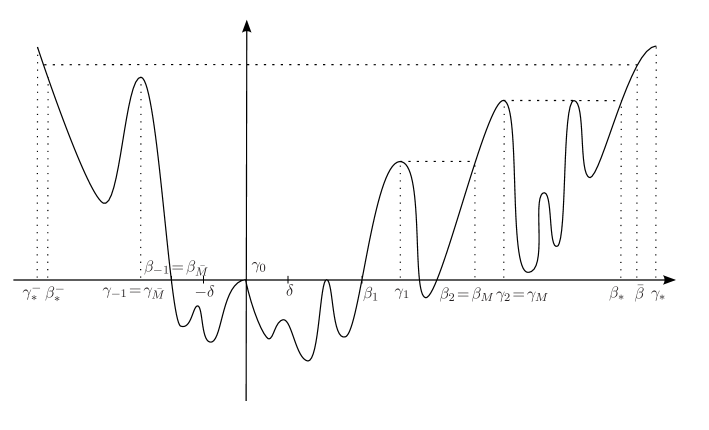
Figure 1. The function $F$

Our main multiplicity results are the following, where from now on $\gamma_{*}=\infty$ in the case that $f$ satisfies assumptions $(A2)$.

Theorem 1.1.

Assume that $f$ satisfies either assumptions $(A1)$ or $(A2)$. Then, there exists $k_{0}\in\mathbb{N}\cup\{0\}$ such that for any $k\geq k_{0}$, there exist at least two solutions $u$ of (1.6), with initial value in $(\beta_{*},\gamma_{*})$, having exactly $k$ sign changes in $(0,\infty)$.

Note that for any $i>1$ there exists $\gamma_{i}^{-}<0$ such that the restriction of $f$ to the interval $(\gamma_{i}^{-},\gamma_{i}]$ satisfies condition $(A1)$, and similarly for $i<-1$. Also, from the results in [15], it follows that for any $k\in\mathbb{N}\cup\{0\}$, there exists at least one solution $u$ of (1.6), with initial value in $(\beta_{1},\gamma_{1})$, having exactly $k$ sign changes in $(0,\infty)$. Hence we immediately obtain the following corollary:

Corollary. Assume that $f$ satisfies either assumptions $(A1)$ or $(A2)$. Then there exists $k_{0}\in\mathbb{N}\cup\{0\}$ such that for any $k\geq k_{0}$, there exist at least $2M+1$ solutions of (1.6) with a positive initial value, and at least $2\bar{M}-1$ solutions of (1.6) with a negative initial value, having exactly $k$ sign changes in $(0,\infty)$.

Our next result shows that bound states with initial value in $(\beta_{*},\gamma_{*})$ need not exist for every $k\in\mathbb{N}\cup\{0\}$:

Theorem 1.2.

Let $\bar{u}$ denote the largest point in $(\beta_{*}^{-},0)$ such that $F(\bar{u})=F(\gamma_{1})$. If either $f$ satisfies assumptions $(A1)$ and

$$-\min_{s\in[\beta_{*}^{-},\beta_{*}]}F(s)<\frac{(\beta_{*}-\gamma_{1})}{2(N-1)(k+1)}\frac{F(\gamma_{1})}{\gamma_{1}-\bar{u}}-F(\gamma_{*}),$$ (1.7)

or $f$ satisfies $(A2)$ and

$$-\min_{s\in[\beta_{*}^{-},\beta_{*}]}F(s)<\frac{(\beta_{*}-\gamma_{1})}{2(N-1)(k+1)}\frac{F(\gamma_{1})}{\gamma_{1}-\bar{u}}-\sup_{s\in[0,\alpha_{k}]}F(s),$$ (1.8)

where $\alpha_{k}$ is defined in Lemma 3.1, then there are no solutions $u$ of (1.6), with initial value in $(\beta_{*},\gamma_{*})$, having exactly $j$ sign changes in $(0,\infty)$ for any $j=0,1,\ldots,k$.

In our last result we give a sufficient condition so that $k_{0}=1$ in Theorem 1.1. In order to state it we define

$$\bar{F}:=-\min_{s\in[0,\beta_{1}]}F(s)>0.$$

$$A=\frac{\beta_{*}-\beta_{1}}{((F(\bar{\beta})-F(\gamma_{M})))^{1/2}}+\Bigl{(}\frac{2N(\bar{\beta}-\beta_{*})}{\min_{t\in[\beta_{*},\bar{\beta}]}f(t)}\Bigr{)}^{1/2}\quad\mbox{and}\quad\bar{I}=F(\gamma_{*}),$$

if $f$ satisfies $(A1)$, and

$$A=\max\{1,\frac{\beta_{*}-\beta_{1}}{((F(\bar{\beta})-F(\gamma_{M})))^{1/2}}+\Bigl{(}\frac{2N(\bar{\beta}-\beta_{*})}{\min_{t\in[\beta_{*},\bar{\beta}]}f(t)}\Bigr{)}^{1/2}\}$$

and

$$\bar{I}:=\Bigl{(}\frac{\bar{C}+1}{\bar{C}}\Bigr{)}^{N}\Bigl{(}2F(\bar{\beta})+(\bar{\beta}-\beta_{1})^{2}+\frac{1}{N}\Bigl{(}\sup_{s\in[\beta_{1},\bar{\beta}]}Q(s)-\min_{s\in[s_{0},\bar{\beta}]}Q(s)\Bigr{)}\Bigr{)}+\frac{(N-2)^{2}\bar{\beta}^{2}}{2\bar{C}^{2}}$$

if $f$ satisfies $(A2)$ where

$$\bar{C}:=2(N-1)\frac{\bar{\beta}-\beta_{1}}{F(\bar{\beta})-F(\gamma_{M})}(2(F(\bar{\beta})-\min_{s\in[\beta_{1},\beta_{*}]}F(s)))^{1/2},$$

We have

Theorem 1.3.

If $f$ satisfies assumptions $(A1)$ or $(A2)$ and

$$(\bar{C}+A)\bar{I}<\frac{2^{1/2}(N-1)}{(\bar{I}+\bar{F})^{1/2}}\int_{0}^{\beta_{1}}|F(s)|ds,$$ (1.9)

then for any $k\in\mathbb{N}\cup\{0\}$ there exist at least two solutions $u$ of (1.6), with initial value in $(\beta_{*},\gamma_{*})$, having exactly $k$ sign changes in $(0,\infty)$.

Remark 1.4.

If $f$ satisfies $(A2)$ and

$$F_{\infty}:=\lim\limits_{s\to\infty}F(s)<\infty,$$

then the above theorem holds with $\bar{I}=F_{\infty}$.

We will obtain our results through a careful study of the initial value problem

$$\begin{gathered}u^{\prime\prime}+\frac{N-1}{r}u^{\prime}+f(u)=0,\quad r>0,\quad N\geq 2,\\ u(0)=\alpha,\quad u^{\prime}(0)=0,\end{gathered}$$ (1.10)

for $\alpha\in(\beta_{*},\gamma_{*})$. By a solution to (1.10) we mean a $C^{1}$ function $u$ such that $u^{\prime}$ is also $C^{1}$ in its domain and we denote such a solution by $u(\cdot,\alpha)$.

The idea of the proof of our multiplicity result is to define the set $\mathcal{Q}_{1}$ as the set of initial values $\alpha>\beta_{*}$ such that the corresponding solution $u(\cdot,\alpha)$ of (1.10) is strictly positive and $\inf_{r>0}u(r,\alpha)\in(0,\beta_{1})$. We extend this definition to the similar sets $\mathcal{Q}_{k}$ when the solution $u(\cdot,\alpha)$ of (1.10) has exactly $k-1$ zeros. By continuous dependence of solutions in the initial data, it will follow that $\mathcal{Q}_{k}$ is an open set. Let $\mathcal{G}_{k}$ be the set of initial values $\alpha>\beta_{*}$ such that the corresponding solution $u(\cdot,\alpha)$ is a solution of (1.6) having exactly $k-1$ simple zeros in $(0,\infty)$.

In some of previous works concerning existence of solutions, see for example [20, 21] for ground states and [15, 16] for higher order bound states having a prescribed number of nodes, the conditions on $f$ imply that $F$ does not possess a positive local maximum, hence $\mathcal{Q}_{k}$ in nonempty for all $k$ and $\sup(\mathcal{Q}_{k}\cup\mathcal{G}_{k})\in\mathcal{G}_{k}$. On the other hand, $\inf(\mathcal{Q}_{k}\cup\mathcal{G}_{k})$ in general does not belong to $\mathcal{G}_{k}$, in fact there are cases for which there is uniqueness, that is, $\mathcal{G}_{k}$ is a singleton.

The presence of a positive local maximum for $F$ ($(f_{3})$ in our assumptions) will guarantee that if $\mathcal{Q}_{k}$ is nonempty, then $\inf(\mathcal{Q}_{k}\cup\mathcal{G}_{k})$ and $\sup(\mathcal{Q}_{k}\cup\mathcal{G}_{k})$ are different and belong to $\mathcal{G}_{k}$. Theorem 1.1 will follow once we have proved that $\mathcal{Q}_{k}$ is nonempty for $k$ large enough. A striking difference with the case for which $F$ does not possess a positive local maximum is that now $\mathcal{Q}_{1}$ can be empty. This result is contained in Theorem 1.2. Finally, in Theorem 1.3 we give conditions on $f$ so that $\mathcal{Q}_{1}\not=\emptyset$.

This paper is organized as follows. In section 2, we establish some properties of the solutions to (1.10), we restrict its domain to the set of unique extendibility, define some crucial sets of initial values and prove some crucial results concerning the solutions having initial value in these sets. Then in section 3 we prove our main result. Finally in the Appendix we prove a non-oscillation result for the solutions of (1.10).

2. Some properties of the solutions of the initial value problem

The aim of this section is to establish several properties of the solutions to the initial value problem (1.10). Since $f$ is continuous, problem (1.10) has a solution defined for all $r\geq 0$ for any $\alpha>\beta_{*}$ but it might not be uniquely defined. It is straight forward to see that unique extendibility can be lost only if $u$ reaches a double zero.

Definition 2.

The domain $D$ of definition of $u$ will be the domain of unique extendibility.

That is, $D=(0,D_{\alpha})$, where if $D_{\alpha}<\infty$, then $D_{\alpha}$ is a double zero of $u$.

By standard theory of ordinary differential equations, the solution depends continuously on the initial data in any compact subset of its domain of definition.

We start by stating without proof the following basic proposition. The proof of $(i)$ and $(iii)$ can be found in [15, Proposition 2.3] and the proof of $(ii)$ can be found in [18, Proposition 3.4]. A proof of $(iv)$ under other assumptions can be found in [16], we include a proof of it under the new assumptions in the Appendix. These proofs are based on properties of the well known energy functional

$$I(r,\alpha)=\frac{|u^{\prime}(r,\alpha)|^{2}}{2}+F(u(r,\alpha))$$

for which we have

$$I^{\prime}(r,\alpha)=-(N-1)\frac{|u^{\prime}(r,\alpha)|^{2}}{r}.$$ (2.1)

Proposition 2.1.

Let $f$ satisfy $(f_{1})$-$(f_{2})$ in either $(A1)$ or $(A2)$ and let $u(\cdot,\alpha)$ be a solution of (1.10).

1. There exists $C(\alpha)>0$ such that $|u(r,\alpha)|+|u^{\prime}(r,\alpha)|\leq C(\alpha)$.

2. $\lim_{r\to\infty}I(r,\alpha)$ exists and is equal to $F(\ell)$, where $\ell$ is a zero of $f$.

3. If $u(\cdot,\alpha)$ is defined in $[0,\infty)$ and $\lim_{r\to\infty}u(r,\alpha)=\ell$, then

   $$\quad\lim_{r\to\infty}u^{\prime}(r,\alpha)=0\quad\mbox{and}\quad\ell\ \mbox{is a zero of $f$}.$$

4. Assume further that $f$ satisfies $(f_{4})$ of either $(A1)$ or $(A2)$. Then $u$ has at most a finite number of sign changes.

Let us set

$$Z_{1}(\alpha):=\sup\{r>0\ |\ u(s,\alpha)>0\mbox{ and }u^{\prime}(s,\alpha)<0\ \mbox{ for all }s\in(0,r)\}$$

and define

$${\mathcal{N}_{1}} = \{\alpha\in[\beta_{*},\gamma_{*})\ :\ u(Z_{1}(\alpha),\alpha)=0\quad\mbox{and}\quad u^{\prime}(Z_{1}(\alpha),\alpha)<0\}$$

$${\mathcal{G}_{1}} = \{\alpha\in[\beta_{*},\gamma_{*})\ :\ u(Z_{1}(\alpha),\alpha)=0\quad\mbox{and}\quad u^{\prime}(Z_{1}(\alpha),\alpha)=0\}$$

$${\mathcal{P}_{1}} = \{\alpha\in[\beta_{*},\gamma_{*})\ :\ u(Z_{1}(\alpha),\alpha)>0\},$$

where $\beta_{*}$ is as defined in Definition 1(ii), and we recall $\gamma_{*}=\infty$ in case $f$ satisfies $(A2)$. We now extend these definitions by induction for $k\geq 2$.

If ${\mathcal{N}_{k-1}}\not=\emptyset$, we set

$${\mathcal{F}}_{k}=\{\alpha\in\mathcal{N}_{k-1}\ :\ (-1)^{k}u^{\prime}(r,\alpha)\leq 0\quad\mbox{for all }r>Z_{k-1}(\alpha)\}.$$

For $\alpha\in\mathcal{N}_{k-1}\setminus{\mathcal{F}}_{k}$, we set

$$T_{k-1}(\alpha): = \sup\{r\in(Z_{k-1}(\alpha),D_{\alpha})\ :\ (-1)^{k}u^{\prime}(r,\alpha)\leq 0\},$$

and for $\alpha\in{\mathcal{F}}_{k}$, we set $T_{k-1}(\alpha)=\infty$.

Next, for $\alpha\in\mathcal{N}_{k-1}\setminus{\mathcal{F}}_{k}$, we define the extended real number

$$Z_{k}(\alpha):=\sup\{r>T_{k-1}(\alpha)\ |\ (-1)^{k}u(s,\alpha)<0\mbox{ and }(-1)^{k}u^{\prime}(s,\alpha)>0\$$

$$\mbox{ for all }s\in(T_{k-1}(\alpha),r)\},$$

and again if $\alpha\in{\mathcal{F}}_{k}$, we set $Z_{k}(\alpha)=\infty$.

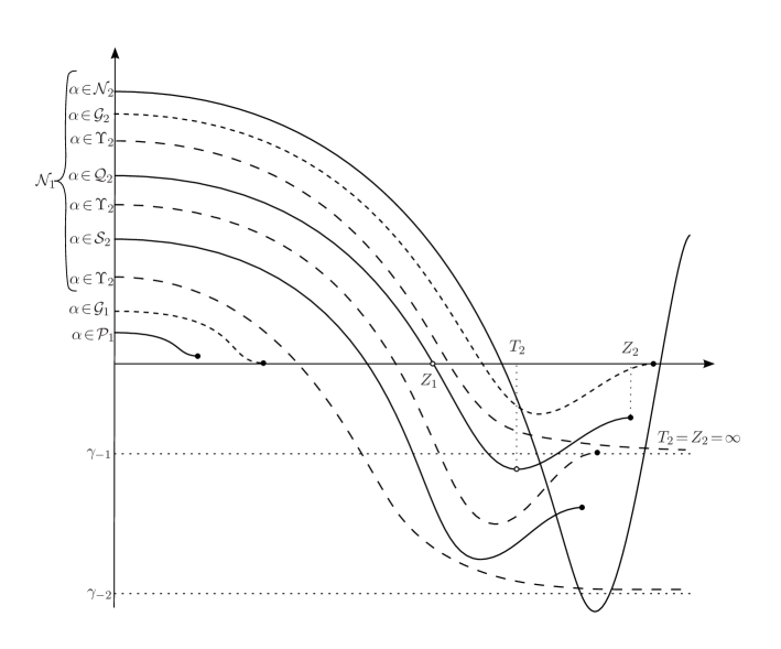
Figure 2. Solutions of (1.10) with initial condition in these sets

We now define

$${\mathcal{N}_{k}} = \{\alpha\in\mathcal{N}_{k-1}\setminus{\mathcal{F}}_{k}\ :\ u(Z_{k}(\alpha),\alpha)=0\quad\mbox{and}\quad(-1)^{k}u^{\prime}(Z_{k}(\alpha),\alpha)>0\},$$

$${\mathcal{G}_{k}} = \{\alpha\in\mathcal{N}_{k-1}\setminus{\mathcal{F}}_{k}\ :\ u(Z_{k}(\alpha),\alpha)=0\quad\mbox{and}\quad u^{\prime}(Z_{k}(\alpha),\alpha)=0\},$$

$${\mathcal{P}_{k}} = \{\alpha\in\mathcal{N}_{k-1}\ :\ (-1)^{k}u(Z_{k}(\alpha),\alpha)<0\}.$$

Finally, for any $k\in\mathbb{N}$ we decompose $\mathcal{P}_{k}$ as follows:

$$\mathcal{P}_{k}=\mathcal{Q}_{k}\cup\mathcal{S}_{k}\cup\Upsilon_{k},$$

where

$$\mathcal{Q}_{k} = \{\alpha\in\mathcal{P}_{k}\ :\ \gamma_{-1}<u(Z_{k}(\alpha),\alpha)<0\quad\mbox{or}\quad 0<u(Z_{k}(\alpha),\alpha)<\gamma_{1}\}$$

$$\mathcal{S}_{k} = \bigcup_{i=\bar{M}-1,\ i\neq 0,-1}^{M}\{\alpha\in\mathcal{P}_{k}\ :\ \gamma_{i}<u(Z_{k}(\alpha),\alpha)<\gamma_{i+1}\}$$

$$\Upsilon_{k} = \bigcup_{i=\bar{M},\ i\neq 0}^{M}\{\alpha\in\mathcal{P}_{k}\ :\ u(Z_{k}(\alpha),\alpha)=\gamma_{i}\}$$

where the constants $\gamma_{i}$ are defined in Definition 1(i).

It should be noticed that if $\alpha\in\Upsilon_{k}$, then necessarily $Z_{k}(\alpha)=\infty$. Indeed, let $\alpha\in\Upsilon_{k}$ and assume $Z_{k}(\alpha)<\infty$. Then $u^{\prime}(Z_{k}(\alpha),\alpha)=0$ and $u(Z_{k}(\alpha),\alpha)=\gamma_{i}$ for some $i\not=0$. By the unique solvability of (1.10) up to a double zero, it must be that $u(r)\equiv\gamma_{i}$ for all $r\geq Z_{k}(\alpha)$. But then we can argue as in the proof of [20, Proposition 1.3.1] to obtain a contradiction to the fact that by the Lipschitz assumption on $f$, we have that

$$\int_{\gamma_{i}}\frac{du}{|F(\gamma_{i})-F(u)|^{1/2}}=\infty.$$

As the minima (maxima) of $u$ occur at values where $f(u)\leq 0$ ($f(u)\geq 0$), it follows that if $\alpha\in\mathcal{S}_{j}\cup\mathcal{Q}_{j}$, with $\gamma_{i}<u(Z_{j}(\alpha),\alpha)<\gamma_{i+1}$, then $F(u(Z_{j}(\alpha),\alpha))<\min\{F(\gamma_{i}),F(\gamma_{i+1})\}$ and hence $\gamma_{i}<u(r,\alpha)<\gamma_{i+1}$ for all $r>Z_{j}(\alpha)$.

The rest of this section is devoted to the proof of some crucial properties of the sets defined above.

Lemma 2.2.

Assume that $f$ satisfies $(A1)$ or $(A2)$ and let $k\in\mathbb{N}$.

1. If $\bar{\alpha}\in\mathcal{G}_{k}$, then there exists a neighborhood $V$ of $\bar{\alpha}$ such that if $\alpha\in V\cap\mathcal{N}_{k}$, then $\alpha\in\mathcal{Q}_{k+1}$

2. If $\bar{\alpha}$ is such that $u(Z_{k}(\bar{\alpha}))=\gamma$, with $\gamma$ a local maximum of $F$ with $F(\gamma)\geq 0$, then there exists a neighborhood $V$ of $\bar{\alpha}$ such that if $\alpha\in V\cap\mathcal{N}_{k}$, then $F(u(T_{k}(\alpha),\alpha))<F(\gamma)$.

3. Let $\bar{\alpha}$ be such that $u(Z_{k}(\bar{\alpha}))=\gamma$, with $\gamma$ a local maximum of $F$ with $F(\gamma)\geq 0$, and $\gamma_{i}<\gamma<\gamma_{i+1}$. Then there exists a neighborhood $V$ of $\bar{\alpha}$, such that if $\alpha\in V$, then $\alpha\in\mathcal{N}_{k-1}\setminus\mathcal{N}_{k}$ and either $u(Z_{k}(\alpha))=\gamma$ or there exists $r_{1}>0$ such that $\gamma_{i}<u(r_{1},\alpha)<\gamma_{i+1}$ and $I(r_{1},\alpha)<\min\{F(\gamma_{i}),F(\gamma_{i+1})\}$.

Proof.

Part $(i)$: Let $\bar{\alpha}\in\mathcal{G}_{k}$. Without loss of generality we may assume that $u(\cdot,\bar{\alpha})$ is decreasing in $(T_{k-1}(\bar{\alpha}),Z_{k}(\bar{\alpha}))$. We will show that there exists a neighborhood $V$ such that if $\alpha\in V\cap\mathcal{N}_{k}$, then $u(T_{k}(\alpha),\alpha)>\beta_{-1}$. Arguing by contradiction we assume that there exists a sequence $\{\alpha_{i}\}$, $\alpha_{i}\to\bar{\alpha}$ with $\alpha_{i}\in\mathcal{N}_{k}$, such that

$$u(T_{k}(\alpha_{i}),\alpha_{i})\leq\beta_{-1}$$ (2.2)

so that $u(\cdot,\alpha_{i})$ has crossed the value $-\delta$ with positive energy.

Let now $\varepsilon\in(0,1)$. Since

$$\lim_{r\to Z_{k}(\bar{\alpha})}I(r,\bar{\alpha})=0\quad\mbox{and}\quad\lim_{r\to Z_{k}(\bar{\alpha})}u(r,\bar{\alpha})=0,$$

there exists $r_{0}>T_{k-1}(\bar{\alpha})$ such that

$$I(r_{0},\bar{\alpha})<\varepsilon,\quad 0<u(r_{0},\bar{\alpha})<\delta/2,$$

where $\delta$ is as defined in $(f_{2})$ of $(A1)$ and $(A2)$, and therefore by continuity, for $i$ large enough, $0<u(r_{0},\alpha_{i})<\delta$, $Z_{k}(\alpha_{i})>r_{0}$, and

$$I(r_{0},\alpha_{i})<2\varepsilon.$$

Since $I$ is decreasing in $r$, we have that

$$I(r,\alpha_{i})<2\varepsilon\quad\mbox{for all}\quad r\in(r_{0},T_{k}(\alpha_{i})),$$

hence,

$$|u^{\prime}(r,\alpha_{i})|\leq\sqrt{4-2\min_{s\in[\beta_{*}^{-},\beta_{*}]}F(s)}:=K\quad\mbox{for all }r\in(r_{0},T_{k}(\alpha_{i}))$$ (2.3)

and $i$ large enough. Let us denote by $r(\cdot,\alpha_{i})$ the inverse of $u(\cdot,\alpha_{i})$ in $(T_{k-1}(\alpha_{i}),T_{k}(\alpha_{i}))$. From (2.2), $[-\delta,0]\subset[u(T_{k}(\alpha_{i}),\alpha_{i}),0]$, and from (2.3), by the mean value theorem we obtain that

$$\Bigl{(}\frac{-\delta}{2},\alpha_{i}\Bigr{)}-r\Bigl{(}\frac{-\delta}{4},\alpha_{i}\Bigr{)}\geq\frac{\delta}{4K}.$$

Let now

$$H(r,\alpha)=r^{2(N-1)}I(r,\alpha).$$

Then

$$H^{\prime}(r,\alpha)=2(N-1)r^{2N-3}F(u(r,\alpha)),$$

implying that for $\alpha=\bar{\alpha}$, $H^{\prime}(r,\bar{\alpha})<0$ for all $r\in(r_{0},Z_{k}(\bar{\alpha}))$ and

$$H(r,\bar{\alpha})\downarrow L\geq 0$$

as $r\to Z_{k}(\bar{\alpha})$. Also, by choosing a larger $r_{0}$ if necessary, we may assume $H(r_{0},\bar{\alpha})<L+\varepsilon$. Thus by continuity we have that

$$H(r_{0},\alpha_{i})\leq L+2\varepsilon\quad\mbox{for $i$ large enough.}$$

Also, as $u(r,\alpha_{i})<\delta$ for $r\in[r_{0},Z_{k}(\alpha_{i})]$, $H$ is decreasing in $[r_{0},Z_{k}(\alpha_{i})]$ implying

$$H(Z_{k}(\alpha_{i}),\alpha_{i})\leq L+2\varepsilon\quad\mbox{for $i$ large enough.}$$

Integrating $H^{\prime}(\cdot,\alpha_{i})$ over $(Z_{k}(\alpha_{i}),r(\frac{-\delta}{2},\alpha_{i}))$, we find that

$$H(r\Bigl{(}\frac{-\delta}{2},\alpha_{i}\Bigr{)},\alpha_{i})-H(Z_{k}(\alpha_{i}),\alpha_{i})=-2(N-1)\int_{Z_{k}(\alpha_{i})}^{r(\frac{-\delta}{2},\alpha_{i})}t^{2N-3}|F(u(t,\alpha_{i}))|dt$$

and thus, observing that since $N\geq 2$, we have $2N-3>0$ implying

$$H(r\Bigl{(}\frac{-\delta}{2},\alpha_{i}\Bigr{)},\alpha_{i}) \leq L+2\varepsilon-2(N-1)(Z_{k}(\alpha_{i}))^{2N-3}\int_{Z_{k}(\alpha_{i})}^{r(\frac{-\delta}{2},\alpha_{i})}|F(u(t,\alpha_{i}))|dt$$

$$\leq L+2\varepsilon-2(N-1)(Z_{k}(\alpha_{i}))^{2N-3}\int_{r(\frac{-\delta}{4},\alpha_{i})}^{r(\frac{-\delta}{2},\alpha_{i})}|F(u(t,\alpha_{i}))|dt$$

$$\leq L+2\varepsilon-2(N-1)(Z_{k}(\alpha_{i}))^{2N-3}(r\Bigl{(}\frac{-\delta}{2},\alpha_{i}\Bigr{)}-r\Bigl{(}\frac{-\delta}{4},\alpha_{i}\Bigr{)})C$$

$$\leq L+2\varepsilon-2(N-1)(Z_{k}(\alpha_{i}))^{2N-3}\frac{\delta}{4K}C,$$

where $C:=\inf\{|F(s)|,\ s\in[\frac{-\delta}{2},\frac{-\delta}{4}]\}$. If $Z_{k}(\bar{\alpha})=\infty$, by taking $i$ larger if necessary, we conclude that $H(r(\frac{-\delta}{2},\alpha_{i}),\alpha_{i})<0$, a contradiction. If $Z_{k}(\bar{\alpha})<\infty$, the same conclusion follows by observing that in this case $L=0$ and $Z_{k}(\alpha_{i})$ is bounded below by the positive constant $r_{1}/2$, where $r_{1}$ the first value of $r>0$ where $u(\cdot,\bar{\alpha})$ takes the value $\delta$.

Part $(ii)$: The proof is very similar to that of Part $(i)$, the only difference is that now we consider

$$\tilde{H}(r,\alpha)=r^{2(N-1)}(I(r,\alpha)-F(\gamma)),$$ (2.4)

so that

$$\tilde{H}^{\prime}(r,\alpha)=2(N-1)r^{2N-3}(F(u(r,\alpha))-F(\gamma)).$$

We still assume that $u(\cdot,\bar{\alpha})$ is decreasing in $(T_{k-1}(\bar{\alpha}),Z_{k}(\bar{\alpha}))$ and that $\{\alpha_{i}\}$ contains a subsequence, still denoted the same, such that

$$F(u(T_{k}(\alpha_{i}),\alpha_{i}))\geq F(\gamma)$$

so that $u(\cdot,\alpha_{i})$ has crossed the value $-\delta$ with energy greater than $F(\gamma)$. As above, $[-\delta,0]\subset[u(T_{k}(\alpha_{i}),\alpha_{i}),0]$, and from the mean value theorem we obtain that

$$r\Bigl{(}\frac{-\delta}{2},\alpha_{i}\Bigr{)}-r\Bigl{(}\frac{-\delta}{4},\alpha_{i}\Bigr{)}\geq\frac{\delta}{4K},$$

where now $K:=\sqrt{2(F(\gamma)+2-2\min_{s\in[\beta_{*}^{-},\beta_{*}]}F(s))}$. Setting $C_{0}:=\inf\{|F(s)-F(\gamma)|,\ s\in[\frac{-\delta}{2},\frac{-\delta}{4}]\}$ and $0\leq L:=\lim\limits_{r\to Z_{k}(\bar{\alpha})}\tilde{H}(r,\bar{\alpha})$, we obtain

$$\tilde{H}(r\Bigl{(}\frac{-\delta}{2},\alpha_{i}\Bigr{)},\alpha_{i})\leq L+2\varepsilon-2(N-1)(Z_{k}(\alpha_{i}))^{2N-3}\frac{\delta}{4K}C_{0}.$$

The same reasoning as above leads to the conclusion that for $i$ sufficiently large

$$I(r\Bigl{(}\frac{-\delta}{2},\alpha_{i}\Bigr{)},\alpha_{i})<F(\gamma),$$

a contradiction to the fact that $I$ is decreasing.

Part $(iii)$: If $\gamma_{i}<\gamma<\gamma_{i+1}$, and since $F(\gamma)\leq\min\{F(\gamma_{i}),F(\gamma_{i+1})\}$, we can repeat the same argument as above but replacing the interval $[-\delta/2,-\delta/4]$ by an interval $[a,b]\subset(\gamma_{i},\gamma)$ if $i\geq 0$ and $[a,b]\subset(\gamma,\gamma_{i+1})$ if $i\leq-1$, where $F(s)<F(\gamma)$. ∎

Our next result is a generalization of Lemma 3.1 in [21].

Lemma 2.3.

1. Let $f$ satisfy $(A1)$ or $(A2)$, and let $\bar{\alpha}$ such that $u(Z_{j}(\bar{\alpha}),\bar{\alpha})=\gamma_{i}$ for some $i\neq 0,\bar{M}-1$, and let $k\geq j$. Then there exists a neighborhood $V_{k}$ of $\bar{\alpha}$ such that if $\alpha\in V_{k}$ and $u(Z_{j}(\alpha),\alpha)\not=\gamma_{i}$, then $\alpha\in\mathcal{N}_{k}$.

2. Let $f$ satisfy $(A2)$, $\bar{\beta}$ be defined as in Definition 1(iii), $\bar{u}\in(\gamma_{*}^{-},0)$ such that $F(\bar{u})=F(2\bar{\beta})$ and set $-\tilde{F}:=\min_{s\in[\beta_{*}^{-},\beta_{*}]}F(s)$. If $\alpha>2\bar{\beta}$, with $\alpha\in\mathcal{N}_{j}$ for $j\leq k$ and

   $$\bar{r}(\alpha)\geq C_{k}:=\frac{(k+1)(2\bar{\beta}-\bar{u})(N-1)\sqrt{2(F(2\bar{\beta})+\tilde{F})}}{F(2\bar{\beta})-F(\bar{\beta})},$$

   where $\bar{r}(\alpha)$ denotes the first point after $T_{j-1}(\alpha)$ for which $F(u(\bar{r}(\alpha),\alpha))=F(2\bar{\beta})$, then $\alpha\in\mathcal{N}_{k}$.

Proof.

Part (i): Without loss of generality we may assume that $u(Z_{j}(\bar{\alpha}),\bar{\alpha})=\gamma_{i}>0$. Let

$$B_{i}=\max\{F(\gamma_{\ell})\ |\ F(\gamma_{\ell})<F(\gamma_{i})\}$$

and $u_{i}$ be the largest point in $(\gamma_{*}^{-},0)$ such that $F(\gamma_{i})=F(u_{i})$. Set

$$\varepsilon:=\frac{F(\gamma_{i})-B_{i}}{k+1}.$$

Let $D_{1},\ D_{2}$ be such that

$$D_{1}:=\frac{(\gamma_{i}-u_{i})(N-1)\sqrt{2(F(\gamma_{i})+\tilde{F})}}{\varepsilon},\quad F(u(D_{2},\bar{\alpha}))>F(\gamma_{i})-\frac{\varepsilon}{2},$$

and set $D:=\max\{D_{1},D_{2}\}$. By the continuous dependence of the solutions on the initial data and Lemma 2.2(ii), there exists a neighborhood $V$ of $\bar{\alpha}$ such that for $\alpha\in V$,

$$\sup_{r\in[0,D]}|F(u(r,\alpha))-F(u(r,\bar{\alpha}))|<\varepsilon/2,$$

and if $\alpha\in\mathcal{N}_{j}$, $F(u(T_{j}(\alpha),\alpha))<F(\gamma_{i})$. Let now $\alpha\in V$ and assume that $u(Z_{j}(\alpha),\alpha)\not=\gamma_{i}$, and denote by $\bar{r}_{\varepsilon}$ the first point after $D$ such that $F(u(\bar{r}_{\varepsilon},\alpha))=F(\gamma_{i})-\varepsilon$. Denote by $r_{0}:=r_{0}(\alpha)$ the first point after $\bar{r}_{\varepsilon}$ where $u^{\prime}(r_{0},\alpha)=0$. By integrating (2.1) over $(\bar{r}_{\varepsilon},r_{0})$ we find that

$$I(\bar{r}_{\varepsilon},\alpha)-F(u(r_{0},\alpha))=(N-1)\int_{\bar{r}_{\varepsilon}}^{r_{0}}\frac{|u^{\prime}(r,\alpha)|^{2}}{r}dr,$$

hence, using that

$$|u^{\prime}(r,\alpha)|\leq\sqrt{2(I(\bar{r}_{\varepsilon})+\tilde{F})}\quad\mbox{for all }r>\bar{r}_{\varepsilon}$$

we obtain

$$F(u(r_{0},\alpha))\geq I(\bar{r}_{\varepsilon})\Bigl{(}1-\frac{\sqrt{2(I(\bar{r}_{\varepsilon})+\tilde{F})}}{I(\bar{r}_{\varepsilon})}\frac{(\gamma_{i}-u_{i})(N-1)}{\bar{r}_{\varepsilon}}\Bigr{)}.$$

Therefore, as $\sqrt{2(I+\tilde{F})}/I$ is decreasing in $I$, $I(\bar{r}_{\varepsilon})\geq F(\gamma_{i})-\varepsilon$, $\bar{r}_{\varepsilon}>D$ and $\varepsilon<F(\gamma_{i})/(k+1)$, we have that

$$F(u(r_{0},\alpha)) \geq I(\bar{r}_{\varepsilon})\Bigl{(}1-\frac{\sqrt{2(F(\gamma_{i})-\varepsilon+\tilde{F})}}{F(\gamma_{i})-\varepsilon}\frac{\varepsilon}{\sqrt{2(F(\gamma_{i})+\tilde{F})}}\Bigr{)}$$

$$\geq F(\gamma_{i})-2\varepsilon.$$

Hence,

$$F(\beta_{i})\leq B_{i}<F(\gamma_{i})-2\varepsilon<F(u(r_{0},\alpha))<F(\gamma_{i}).$$

Since $f(s)>0$ for $s\in(\beta_{i},\gamma_{i})$, we deduce that $r_{0}=T_{j}(\alpha)$. Iterating this process at $\bar{r}_{2\varepsilon}$, the first point after $T_{j}(\alpha)$ at which $F(u(\bar{r}_{2\varepsilon},\alpha))=F(\gamma_{i})-2\varepsilon$, we obtain $\alpha\in\mathcal{N}_{2}$. We repeat this procedure $k$ times to obtain $\alpha\in\mathcal{N}_{k}$.

Part (ii): Without loss of generality we may assume that $u(\bar{r}(\alpha),\alpha)>0$. Let

$$\varepsilon:=\frac{F(2\bar{\beta})-F(\bar{\beta})}{k+1},$$

and again denote by $r_{0}:=r_{0}(\alpha)$ the first point after $\bar{r}(\alpha)$ where $u^{\prime}(r_{0},\alpha)=0$. By integrating (2.1) over $(\bar{r}(\alpha),r_{0})$ as in Part $(i)$ we obtain

$$F(\bar{\beta})<F(2\bar{\beta})-\varepsilon<F(u(r_{0},\alpha)),$$

and therefore $r_{0}=T_{j}(\alpha)$. Iterating this process at $\bar{r}_{\varepsilon}$, the first point after $T_{j}(\alpha)$ at which $F(u(\bar{r}_{\varepsilon},\alpha))=F(\gamma_{i})-\varepsilon$, we obtain $\alpha\in\mathcal{N}_{2}$. We repeat this procedure $k$ times to obtain $\alpha\in\mathcal{N}_{k}$. ∎

Lemma 2.4.

1. The sets ${\mathcal{N}_{k}}$, ${\mathcal{Q}_{k}}$ and ${\mathcal{S}_{k}}$ are open in $[\beta_{*},\gamma_{*})$.

2. The boundary of $\mathcal{G}_{k}\cup\mathcal{Q}_{k}$ is contained in $\bigcup_{i=1}^{k}\mathcal{G}_{i}$.

Proof.

Part (i): The proof that $\mathcal{N}_{k}$ is open follows by continuous dependence of solutions in the initial value $\alpha$, see [15, Proposition 2.4].

Let now $k\geq 1$ and let $\bar{\alpha}\in\mathcal{Q}_{k}$. Without loss of generality we may assume $0<u(Z_{k}(\bar{\alpha}),\bar{\alpha})<\gamma_{1}$. If $I(Z_{k}(\bar{\alpha}),\bar{\alpha})<0$, then there exists $r_{1}>0$ such that $I(r_{1},\bar{\alpha})<0$ and $0<u(r_{1},\bar{\alpha})<\gamma_{1}$. By continuous dependence of solutions in the initial data, there exists $\delta>0$ such that for any $\alpha\in(\bar{\alpha}-\delta,\bar{\alpha}+\delta)$, then $I(r_{1},\alpha)<0$ and $0<u(r_{1},\alpha)<\gamma_{1}$. Moreover, by taking a smaller $\delta$ if necessary, we have that $u(\cdot,\alpha)$ has exactly $k-1$ zeros in $[0,r_{1}]$, hence $(\bar{\alpha}-\delta,\bar{\alpha}+\delta)\subset\mathcal{Q}_{k}$.
If $I(Z_{k}(\bar{\alpha}),\bar{\alpha})=0$, then $u(Z_{k}(\bar{\alpha}),\bar{\alpha})$ is a local maximum of $F$ and the result follows from Lemma 2.2 (iii).
The same argument shows that $\mathcal{S}_{k}$ is open.

Part (ii): As $\mathcal{N}_{k}$ is open, we have that $\mathcal{N}_{k}\cap\overline{\mathcal{Q}_{k}\cup\mathcal{G}_{k}}=\emptyset$.

Let $\bar{\alpha}$ belong to the boundary of $\mathcal{Q}_{k}\cup\mathcal{G}_{k}$. As $\mathcal{Q}_{i}$ and $\mathcal{S}_{i}$ are open, we must have that $\bar{\alpha}\in\bigcup_{i=1}^{k}\mathcal{G}_{i}\cup\Upsilon_{i}$. But from Lemma 2.3, if $\bar{\alpha}\in\bigcup_{i=1}^{k}\Upsilon_{i}$, then there exists $\delta>0$ such that $V_{\delta}(\bar{\alpha})\subset\Upsilon_{j}\cup\mathcal{N}_{k}$, implying that $(\mathcal{Q}_{k}\cup\mathcal{G}_{k})\cap V_{\delta}(\bar{\alpha})=\emptyset$, a contradiction. Hence $\bar{\alpha}\in\bigcup_{i=1}^{k}\mathcal{G}_{i}$. ∎

3. Proof of the main results

In this section we prove our theorems. To this end, we need the following key result, which is a generalization of Lemma 3.1 in [15].

Lemma 3.1.

Assume that $f$ satisfies $(A1)$ or $(A2)$. Then, for each $k\in\mathbb{N}$, there exists $\alpha_{k}\in(\beta_{*},\gamma_{*})$ such that $[\alpha_{k},\gamma_{*})\subset{\mathcal{N}}_{k}$.

Proof.

Assume first that $f$ satisfies $(A1)$. We apply Lemma 2.3 to $\bar{\alpha}=\gamma_{*}$, $\gamma_{i}=\gamma_{*}$ and $j=1$ to obtain that there exists $\alpha_{k}>0$ such that $[\alpha_{k},\gamma_{*})\subset\mathcal{N}_{k}$.

Let $f$ satisfy $(A2)$. We will use here a useful and well known Pohozaev type identity which plays a key role in this proof. For a solution $u(\cdot,\alpha)$ of (1.10), set

$$E(r,\alpha):=2r^{N}I(r,\alpha)+(N-2)r^{N-1}u^{\prime}(r,\alpha)u(r,\alpha).$$

Then

$$E^{\prime}(r,\alpha)=r^{N-1}Q(u(r,\alpha)).$$ (3.1)

Let $k\in\mathbb{N}$, let $\bar{\beta}$ be as defined in Definition 1(iii). By Lemma 2.3(ii), if for $\alpha>2\bar{\beta}$ it holds that $\bar{r}:=\bar{r}(\alpha)\geq C_{k}$, then $\alpha\in\mathcal{N}_{k}$.

Assume that $\alpha\geq 2\bar{\beta}$ and $\bar{r}(\alpha)<C_{k}$. Let $\theta\in(0,1)$ be as in assumption $(f_{5})$ and let $\alpha$ be large enough to have $\theta\alpha>2\bar{\beta}$. By setting $r_{\theta}>0$ the first point where $u(r_{\theta},\alpha)=\theta\alpha$, integration of (3.1) over $[0,\bar{r}]$ yields

$$E(\bar{r},\alpha) \geq (\int_{0}^{r_{\theta}}+\int_{r_{\theta}}^{\bar{r}})t^{N-1}Q(u(t,\alpha))dt$$

$$\geq \int_{0}^{r_{\theta}}t^{N-1}Q(u(t,\alpha))dt\quad\mbox{ (as $Q(u(t,\alpha))\geq 0$ in $[r_{\theta},\bar{r}]$) }$$

$$\geq Q(s_{2})\frac{r_{\theta}^{N}}{N}\quad\mbox{ where we have set $Q(s_{2})=\min_{s\in[\theta\alpha,\alpha]}Q(s)$.}$$

Now we estimate $r_{\theta}$: Set $f(s_{1})=\max_{s\in[\theta\alpha,\alpha]}f(s)$ ($s_{1}\in[\theta\alpha,\alpha]$). From the equation in (1.10), we obtain, as in [15]

$$r_{\theta}\geq\Bigl{(}\frac{c\alpha}{f(s_{1})}\Bigr{)}^{1/2},$$

where $c=2N(1-\theta)$. Therefore, by $(f_{5})$ we conclude that

$$E(\bar{r},\alpha)\geq\frac{1}{N}Q(s_{2})\Bigl{(}\frac{c\alpha}{f(s_{1})}\Bigr{)}^{N/2}\to\infty\mbox{ as $\alpha\to\infty$.}$$

Let us choose $\alpha_{k}$ such that for $\alpha>\alpha_{k}$,

$$E(\bar{r},\alpha)\geq 2(C_{k}+1)^{N}B+(k+1)\bar{Q}\frac{(C_{k}+1)^{N}}{N}$$

where $\bar{Q}:=-\min_{s\in[s_{0},\bar{\beta}]}Q(s)\geq 0$, let $\bar{u}$ be the unique point in $(\gamma_{*}^{-},0)$ such that $F(\bar{u})=F(2\bar{\beta})$ and set

$$B=\Bigl{(}4\bar{\beta}-2\bar{u}+\frac{(N-2)|\bar{u}|}{2(C_{k}+1)}\Bigr{)}^{2}+F(2\bar{\beta}).$$

Let now $\alpha\geq\alpha_{k}$ and let $r_{0}=r_{0}(\alpha)$ be the first point after $\bar{r}(\alpha)$ such that either

$$r_{0}=C_{k}+1,\quad\mbox{or}\quad u^{\prime}(r_{0},\alpha)=0,\quad\mbox{or}\quad F(u(r_{0},\alpha))=F(2\bar{\beta}).$$

As $r_{0}\leq C_{k}+1$, for $r\leq r_{0}$ we have

$$E(r,\alpha) = E(\bar{r},\alpha)+\int_{2\bar{\beta}}^{r}t^{N-1}Q(u(t,\alpha))dt$$

$$\geq E(\bar{r},\alpha)-\bar{Q}\frac{(C_{k}+1)^{N}}{N}.$$

implying

$$E(r,\alpha)\geq 2(C_{k}+1)^{N}B+k\bar{Q}\frac{(C_{k}+1)^{N}}{N}$$ (3.2)

and thus

$$2I(r,\alpha)+\frac{(N-2)|\bar{u}|}{C_{k}+1}|u^{\prime}(r,\alpha)|\geq 2B.$$

We deduce that

$$\Bigl{(}|u^{\prime}(r,\alpha)|+\frac{(N-2)|\bar{u}|}{2(C_{k}+1)}\Bigr{)}^{2} \geq |u^{\prime}(r,\alpha)|^{2}+\frac{(N-2)|\bar{u}||u^{\prime}(r,\alpha)|}{C_{k}+1}$$

$$\geq 2B-2F(\bar{u})=\Bigl{(}4\bar{\beta}-2\bar{u}+\frac{(N-2)|\bar{u}|}{2(C_{k}+1)}\Bigr{)}^{2},$$

hence

$$|u^{\prime}(r,\alpha)|\geq 4\bar{\beta}-2\bar{u}>0$$

thus $u^{\prime}(r_{0},\alpha)\not=0$. Integrating this last inequality over $(\bar{r},r_{0})$ and using that $u(r_{0},\alpha)\geq\bar{u}$, we deduce

$$r_{0}\leq C_{k}+\frac{1}{2}.$$

Hence $F(u(r_{0},\alpha))=F(2\bar{\beta})$, $u(r_{0},\alpha)=\bar{u}$, implying $\alpha\in\mathcal{N}_{1}$, and by (3.2),

$$E(r_{0},\alpha)\geq 2(C_{k}+1)^{N}B+k\bar{Q}\frac{(C_{k}+1)^{N}}{N}$$

Therefore $T_{1}(\alpha)<\infty$, $u(T_{1}(\alpha))<\bar{u}$ and $f(s)<0$ for $u(T_{1}(\alpha))\leq s\leq\bar{u}$, so there exists a first point $r^{+}_{0}$ after $T_{1}(\alpha)$ at which $u$ takes the value $\bar{u}$. If this point is greater than $C_{k}$, we are done. As $E(r_{0}^{+},\alpha)\geq E(r_{0},\alpha)$, we can repeat the above argument as many times as necessary to conclude $\alpha\in\mathcal{N}_{k}$. ∎

Proof of Theorem 1.1.

We first observe that for each $k\in\mathbb{N}\cup\{0\}$, $\mathcal{G}_{k}\cup\mathcal{Q}_{k}$ is bounded by $\alpha_{k+1}$ in Lemma 3.1. We will prove next that there exists $m\in\mathbb{N}\cup\{0\}$ such that $\mathcal{G}_{m}\not=\emptyset$. Once we have done this, we shall denote by $m_{1}$ the first value of $m$ such that $\mathcal{G}_{m}\not=\emptyset$ and set

$$\alpha_{m_{1}}^{\#}:=\inf(\mathcal{G}_{m_{1}}\cup\mathcal{Q}_{m_{1}})\quad\mbox{and}\quad\alpha_{m_{1}}^{*}:=\sup(\mathcal{G}_{m_{1}}\cup\mathcal{Q}_{m_{1}}).$$

Then by Lemma 2.4(ii) and the definition of $m_{1}$, $\alpha_{m_{1}}^{\#},\alpha_{m_{1}}^{*}\in\mathcal{G}_{m_{1}}$. At this point, we cannot guarantee that $\alpha_{m_{1}}^{\#}<\alpha_{m_{1}}^{*}$. As by continuous dependence, for $\bar{\alpha}\in\mathcal{G}_{m_{1}}$ there is a neighborhood of $\bar{\alpha}$ which is contained in $\mathcal{G}_{m_{1}}\cup\mathcal{Q}_{m_{1}}\cup\mathcal{N}_{m_{1}}$. From the definition of $\alpha_{m_{1}}^{\#}$ and $\alpha_{m_{1}}^{*}$, there exists $\delta>0$ such that $(\alpha_{m_{1}}^{\#}-\delta,\alpha_{m_{1}}^{\#})\subset\mathcal{N}_{m_{1}}$ and $(\alpha_{m_{1}}^{*},\alpha_{m_{1}}^{*}+\delta)\subset\mathcal{N}_{m_{1}}$. Hence from Lemma 2.2(i), by taking a smaller $\delta>0$ if necessary, we may assume that $(\alpha_{m_{1}}^{\#}-\delta,\alpha_{m_{1}}^{\#})\subset\mathcal{Q}_{m_{1}+1}$ and $(\alpha_{m_{1}}^{*},\alpha_{m_{1}}^{*}+\delta)\subset\mathcal{Q}_{m_{1}+1}$. Set now

$$\alpha_{m_{1}+1}^{\#}=\inf(\mathcal{G}_{m_{1}+1}\cup Q_{m_{1}+1})\quad\mbox{and}\quad\alpha_{m_{1}+1}^{*}=\sup(\mathcal{G}_{m_{1}+1}\cup Q_{m_{1}+1}).$$

From Lemma 2.4(i), $\alpha_{m_{1}+1}^{\#}<\alpha_{m_{1}+1}^{*}$, and from Lemma 2.4(ii), $\alpha_{m_{1}+1}^{\#}$ and $\alpha_{m_{1}+1}^{*}$ belong to $\mathcal{G}_{m_{1}+1}$. We proceed by induction. At each step $k\geq m_{1}+1$, by Lemma 2.2(i) we have that $\mathcal{Q}_{k}\not=\emptyset$ so we can define

$$\alpha_{k}^{\#}=\inf(\mathcal{G}_{k}\cup Q_{k})\quad\mbox{and}\quad\alpha_{k}^{*}=\sup(\mathcal{G}_{k}\cup Q_{k})$$

to obtain the existence of two different elements in $\mathcal{G}_{k}$ for every $k\geq m_{1}+1$.

We prove next that there exists $m\in\mathbb{N}\cup\{0\}$ such that $\mathcal{G}_{m}\not=\emptyset$. From Lemma 3.1, set

$$\alpha^{1}:=\inf\{\alpha\geq\beta_{*}\ |\ (\alpha,\gamma_{*})\subset\mathcal{N}_{1}\}.$$

Then, by Lemma 2.4(i), either $\alpha^{1}\in\mathcal{G}_{1}$ or $\alpha^{1}\in\Upsilon_{1}$. In our next arguments, and when both cases are possible, we will assume the worse, that is, that the limit points that we obtain are not in $\mathcal{G}_{k}$.
Hence we assume that $\alpha^{1}\in\Upsilon_{1}$. Then there exists $i\in\{1,\ldots,M\}$ such that $u(Z_{1}(\alpha^{1}),\alpha^{1})=\gamma_{i}$. From Lemma 2.3 and the definition of $\alpha^{1}$, for any $k\in\mathbb{N}$,

$$\{\alpha\geq\beta_{*}\ |\ (\alpha^{1},\alpha)\subset\mathcal{N}_{k}\}\not=\emptyset.$$

Since $\alpha^{1}<\gamma_{*}$, we can choose $d>0$ such that $\alpha^{1}+d<\gamma_{*}$ and set, for both sets of assumptions,

$$\alpha^{1}_{k}:=\sup\{\alpha\in(\alpha^{1},\alpha^{1}+d)\ |\ (\alpha^{1},\alpha)\subset\mathcal{N}_{k}\}.$$

As $\{\alpha^{1}_{k}\}$ is monotone decreasing in $k$, it converges. Since (1.10) does not have oscillatory solutions, see Proposition 2.1(iv), it follows that it converges to $\alpha^{1}$. Hence there exists $k_{1}>0$ such that

$$\alpha_{k_{1}}^{1}<\alpha_{k_{1}-1}^{1}<\alpha^{1}+d\quad\mbox{and}\quad u(Z_{k_{1}},\alpha_{k_{1}}^{1})=\gamma_{j},$$

with $F(\gamma_{j})<F(\gamma_{i})$ by Lemma 2.2(ii). We observe that by the strict inequality $\alpha_{k_{1}}^{1}<\alpha_{k_{1}-1}^{1}$, it holds that $\alpha^{1}_{k_{1}}\in\mathcal{N}_{k_{1}-1}$ and $(\alpha^{1},\alpha^{1}_{k_{1}})\subset\mathcal{N}_{k_{1}}$. Set, for $k\geq k_{1}$,

$$\alpha^{2}_{k}:=\inf\{\alpha\in(\alpha^{1},\alpha_{k_{1}}^{1})\ |\ (\alpha,\alpha_{k_{1}}^{1})\subset\mathcal{N}_{k}\}.$$

Now the sequence $\{\alpha^{2}_{k}\}$ is monotone increasing in $k$ and the same argument yields $\alpha_{k}^{2}\to\alpha^{1}_{k_{1}}$ as $k\to\infty$ and there exists $k_{2}>k_{1}$ such that

$$\alpha^{2}_{k_{2}-1}<\alpha^{2}_{k_{2}}$$

so that $\alpha^{2}_{k_{2}}\in\mathcal{N}_{k_{2}-1}$, $(\alpha_{k_{2}}^{2},\alpha^{1}_{k_{1}})\subset\mathcal{N}_{k_{2}}$, and $u(Z_{k_{2}},\alpha_{k_{2}}^{2})=\gamma_{\ell}$ with $F(\gamma_{\ell})<F(\gamma_{j})$, again by Lemma 2.2(ii). We may continue in this way by setting, for $k\geq k_{2}$,

$$\alpha^{3}_{k}:=\sup\{\alpha\in(\alpha_{k_{2}}^{2},\alpha_{k_{1}}^{1})\ |\ (\alpha_{k_{2}}^{2},\alpha)\subset\mathcal{N}_{k}\}.$$

After a finite number of steps we will reach $\gamma_{0}$ obtaining an $\alpha\in\mathcal{G}_{k_{m}}$ for some $k_{m}\in\mathbb{N}$. ∎

Proof of Theorem 1.2.

We prove it first for the case that $f$ satisfies $(A1)$. Assume by contradiction that there exists $\alpha>\beta_{*}$ in $\mathcal{G}_{j}$, that is $u(\cdot,\alpha)$ has $j-1$ sign changes, for some $j=1,\ldots,k+1$. As $u(\cdot,\alpha)$ crosses the value $\gamma_{1}$ at a first point $r_{\gamma_{1}}^{1}$, from $|u^{\prime}(r)|\leq(2(F(\gamma_{*})+\tilde{F}))^{1/2}$ for all $r\leq r_{\gamma_{1}}^{1}$, we find that

$$r_{\gamma_{1}}^{1}\geq\frac{\beta_{*}-\gamma_{1}}{(2(F(\gamma_{*})+\tilde{F}))^{1/2}},$$

where $\tilde{F}$ is defined in Lemma 2.3. Let $r_{\gamma_{1}}\geq r_{\gamma_{1}}^{1}$ denote the last point at which $F(u(r_{\gamma_{1}}))=F(\gamma_{1})$, and we may assume it happens after $T_{i}$, for some $0\leq i<j$. Using that $I(Z_{j})=0$, we find that

$$I(r_{\gamma_{1}}) = (N-1)\int_{r_{\gamma_{1}}}^{Z_{j}}\frac{|u^{\prime}|^{2}}{r}dr$$

$$\leq \frac{N-1}{r_{\gamma_{1}}}(2(F(\gamma_{*})+\tilde{F}))^{1/2}\int_{r_{\gamma_{1}}}^{Z_{j}}|u^{\prime}(r)|dr$$

$$= \frac{N-1}{r_{\gamma_{1}}}(2(F(\gamma_{*})+\tilde{F}))^{1/2}\Bigl{(}\int_{r_{\gamma_{1}}}^{T_{i+1}}|u^{\prime}(r)|dr+\int_{T_{i+1}}^{T_{i+2}}|u^{\prime}(r)|dr+\cdots\int_{T_{j-1}}^{Z_{j}}|u^{\prime}(r)|dr\Bigr{)}$$

$$\leq \frac{(N-1)2(F(\gamma_{*})+\tilde{F})}{\beta_{*}-\gamma_{1}}(j-i)(\gamma_{1}-\bar{u}),$$

we find that

$$F(\gamma_{1})\leq(N-1)2(F(\gamma_{*})+\tilde{F})\frac{j(\gamma_{1}-\bar{u})}{\beta_{*}-\gamma_{1}},$$

a contradiction to (1.7).

If $f$ satisfies $(A2)$, we let $\alpha_{k}$ be as defined in Lemma 3.1. Then we only have to prove that there cannot exist solutions to (1.6) with initial value $\alpha<\alpha_{k}$. But then, as $|u^{\prime}(r)|\leq(2(\sup_{s\in[0,\alpha_{k}]}F(s)+\tilde{F}))^{1/2}$ for all $r>0$, we can argue as above to obtain contradiction to (1.8). ∎

In order to prove our last result, we need the following lemma, which is another generalization of [21, Lemma 3.1].

Lemma 3.2.

Let $f$ satisfy either $(A1)$or $(A2)$, $\bar{\beta}$ be as in Definition 1(iii), and $\alpha>\bar{\beta}$. Let $r_{\bar{\beta}}$ be the first point at which $u(r_{\bar{\beta}},\alpha)=\bar{\beta}$. If

$$r_{\bar{\beta}}\geq\bar{C}:=2(N-1)\frac{\bar{\beta}-\beta_{1}}{F(\bar{\beta})-F(\gamma_{M})}(2(F(\bar{\beta})+\hat{F}))^{1/2},$$

where $\hat{F}:=-\min_{s\in[\beta_{1},\beta_{*}]}F(s)$, then there exists a first point $r_{\beta_{1}}>r_{\bar{\beta}}$ such that $u(r_{\beta_{1}},\alpha)=\beta_{1}$, $u^{\prime}(r_{\beta_{1}},\alpha)<0$, and

$$r_{\beta_{1}}-r_{\bar{\beta}}\leq\frac{\beta_{*}-\beta_{1}}{(F(\bar{\beta})-F(\gamma_{M}))^{1/2}}+\Bigl{(}\frac{2N(\bar{\beta}-\beta_{*})}{\min\limits_{t\in[\beta_{*},\bar{\beta}]}f(t)}\Bigr{)}^{1/2}.$$

Proof.

As any solution satisfying $\alpha>\beta_{*}$ must cross $\beta_{*}$ at a first point that we denote by $r_{\beta_{*}}$, we integrate (2.1) over $[r_{\bar{\beta}},r]$ with $r>r_{\beta_{*}}$, and obtain

$$I(r)=I(r_{\bar{\beta}})-(N-1)\int_{r_{\bar{\beta}}}^{r}\frac{|u^{\prime}(t)|^{2}}{t}dt.$$

Since $|u^{\prime}(r)|\leq 2^{1/2}(I(r_{\bar{\beta}})+\hat{F})^{1/2}$ as long as $u(r)\geq\beta_{1}$, we find that

$$I(r)\geq I(r_{\bar{\beta}})\Bigl{(}1-\frac{\sqrt{2(I(r_{\bar{\beta}})+\hat{F})}}{I(r_{\bar{\beta}})}\frac{(N-1)(\bar{\beta}-u(r))}{r_{\bar{\beta}}}\Bigr{)}.$$

As as $\sqrt{2(I+\tilde{F})}/I$ is decreasing in $I$, $I(r_{\bar{\beta}})\geq F(\bar{\beta})$, and $r_{\bar{\beta}}\geq\bar{C}$, we find that

$$I(r) \geq I(r_{\bar{\beta}})\Bigl{(}1-\frac{F(\bar{\beta})-F(\gamma_{M})}{2F(\bar{\beta})}\Bigr{)}\geq\frac{F(\bar{\beta})+F(\gamma_{M})}{2}$$

$$\geq F(u(r))+\frac{F(\bar{\beta})-F(\gamma_{M})}{2},$$

implying that as long as $\beta_{*}\geq u(r)\geq\beta_{1}$,

$$|u^{\prime}(r)|\geq\bigl{(}F(\bar{\beta})-F(\gamma_{M})\bigr{)}^{1/2}.$$

Hence $u(Z_{1})<\beta_{1}$, and

$$\beta_{*}-\beta_{1}\geq\bigl{(}F(\bar{\beta})-F(\gamma_{M})\bigr{)}^{1/2}(r_{\beta_{1}}-r_{\beta_{*}}).$$

Finally, by integrating the equation in (1.10) over $[r_{\bar{\beta}},r]$ with $r\leq r_{\beta_{*}}$ we find that

$$r^{N-1}|u^{\prime}(r)|=\int_{r_{\bar{\beta}}}^{r}t^{N-1}f(u(t))dt\geq\min_{s\in[\beta_{*},\bar{\beta}]}f(s)\frac{r^{N}-r_{\bar{\beta}}^{N}}{N},$$

hence

$$|u^{\prime}(r)|\geq\Bigl{(}\frac{\min_{s\in[\beta_{*},\bar{\beta}]}f(s)}{N}\Bigr{)}(r-r_{\bar{\beta}}),$$

implying that

$$2(\bar{\beta}-\beta_{*})\geq\Bigl{(}\frac{\min_{s\in[\beta_{*},\bar{\beta}]}f(s)}{N}\Bigr{)}(r_{\beta_{*}}-r_{\bar{\beta}})^{2},$$

hence the result follows. ∎

Proof of Theorem 1.3.

To prove this theorem we only need to prove than under its assumptions, $\mathcal{Q}_{1}\not=\emptyset$. Setting

$$\alpha_{1}^{\#}:=\inf(\mathcal{G}_{1}\cup\mathcal{Q}_{1})\quad\mbox{and}\quad\alpha_{1}^{*}:=\sup(\mathcal{G}_{1}\cup\mathcal{Q}_{1}),$$

and observing that from Lemma (2.4)(i) $\alpha_{1}^{\#}<\alpha_{1}^{*}$ we may argue as in the proof of Theorem 1.1 to obtain the desired result.

Let $\alpha^{*}>\beta_{*}$ be such that $u(\cdot,\alpha^{*})=u(\cdot)$ crosses the value $\beta_{1}$. For simplicity of notation we will set $Z_{1}=Z_{1}(\alpha^{*})$, $I(Z_{1})=I(Z_{1},\alpha^{*})$ and $I(r_{\beta_{1}})=I(r_{\beta_{1}},\alpha^{*})$. As $|u^{\prime}(r)|\leq\sqrt{2(I(r_{\beta_{1}})+\bar{F})}$ for $r\in(r_{\beta_{1}},Z_{1})$, by integrating (2.1) we have

$$Z_{1}^{2(N-1)}I(Z_{1}) = r_{\beta_{1}}^{2(N-1)}I(r_{\beta_{1}})-2(N-1)\int_{r_{\beta_{1}}}^{Z_{1}}r^{2N-3}|F(u(r))|dr$$

$$\leq r_{\beta_{1}}^{2(N-1)}I(r_{\beta_{1}})-2(N-1)r_{\beta_{1}}^{2N-3}\int_{r_{\beta_{1}}}^{Z_{1}}|F(u(r))|dr$$

$$\leq r_{\beta_{1}}^{2(N-1)}I(r_{\beta_{1}})-\frac{2(N-1)r_{\beta_{1}}^{2N-3}}{(2(I(r_{\beta_{1}})+\bar{F}))^{1/2}}\int_{r_{\beta_{1}}}^{Z_{1}}|F(u(r))u^{\prime}(r)|dr$$

$$\leq r_{\beta_{1}}^{2N-3}\Bigl{(}r_{\beta_{1}}I(r_{\beta_{1}})-\frac{2(N-1)}{(2(I(r_{\beta_{1}})+\bar{F}))^{1/2}}\int_{0}^{\beta_{1}}|F(s)|ds\Bigr{)}.$$

Hence, if

$$r_{\beta_{1}}I(r_{\beta_{1}})<\frac{2(N-1)}{(2(I(r_{\beta_{1}})+\bar{F}))^{1/2}}\int_{0}^{\beta_{1}}|F(s)|ds,$$ (3.3)

then $\alpha^{*}\in\mathcal{Q}_{1}$. The proof of this theorem consists in finding an $\alpha^{*}$ such that $u(\cdot,\alpha^{*})$ crosses $\beta_{1}$ and (3.3) holds

In what follows, $\bar{C}$ is as in Lemma 3.2.

If $\gamma_{*}<\infty$, and as $f(\gamma_{*})=0$, by continuous dependence of the solution of (1.10) in the initial data, we have that $r_{\bar{\beta}}(\alpha)\to\infty$ as $\alpha\to\gamma_{*}$, hence we can choose $\alpha^{*}>\beta_{*}$ so that $r_{\bar{\beta}}(\alpha^{*})=\bar{C}$. Using now that $I(r)\leq F(\gamma_{*})$, we see that from (1.9), $\alpha^{*}\in\mathcal{Q}_{1}$.

Let now $\gamma_{*}=\infty$. and set

$$M:=(\bar{C}+1)^{N}\Bigl{(}2F(\bar{\beta})+(\bar{\beta}-\beta_{1})^{2}+\frac{\bar{Q}}{N}\Bigr{)},$$

where $\bar{Q}:=-\min_{s\in[s_{0},\bar{\beta}]}Q(s)\geq 0$. Using the same argument used in the proof of Lemma 3.1, we have that

$$\lim_{\alpha\to\infty}E(r_{\bar{\beta}}(\alpha),\alpha)=\infty.$$

Since $E(r_{\bar{\beta}}(\bar{\beta}),\bar{\beta})=0$, by continuity there exists a smallest $\bar{\alpha}>\bar{\beta}$ such that $E(r_{\bar{\beta}}(\bar{\alpha}),\bar{\alpha})=M$.

If $r_{\bar{\beta}}(\bar{\alpha})\geq\bar{C}$, then again by continuity we can choose $\alpha^{*}\leq\bar{\alpha}$ such that $r_{\bar{\beta}}(\alpha^{*})=\bar{C}$. Moreover, since $E(r_{\bar{\beta}}(\alpha^{*}),\alpha^{*})\leq M$, we find that

$$I(r_{\bar{\beta}}(\alpha^{*}))-\frac{(N-2)\bar{\beta}}{2^{1/2}\bar{C}}(I(r_{\bar{\beta}}(\alpha^{*})))^{1/2}\leq\frac{M}{2\bar{C}^{N}}$$

and hence

$$I(r_{\bar{\beta}}(\alpha^{*}))\leq\frac{(N-2)^{2}\bar{\beta}^{2}}{2\bar{C}^{2}}+\frac{M}{\bar{C}^{N}}.$$

hence, using $I(r_{\beta_{1}})\leq I(r_{\bar{\beta}})$ and assumption (1.9) we obtain that (3.3) holds and thus $\alpha^{*}\in\mathcal{Q}_{1}$.

Let now $r_{\bar{\beta}}(\bar{\alpha})<\bar{C}$. We will first prove that in this case $u=u(\cdot,\bar{\alpha})$ crosses the value $\beta_{1}$ and $r_{\beta_{1}}(\bar{\alpha})<\bar{C}+1$.

Let $r_{0}=r_{0}(\bar{\alpha})$ be the first point after $\bar{r}(\bar{\alpha})$ such that either

$$r_{0}=\bar{C}+1,\quad\mbox{or}\quad u^{\prime}(r_{0},\bar{\alpha})=0,\quad\mbox{or}\quad u(r_{0},\bar{\alpha}))=\beta_{1}.$$

Integrating (3.1) over $[0,r]$ with $r\leq r_{0}$ we get

$$2r^{N}I(r) \geq \int_{0}^{r}t^{N-1}Q(u(t))dt$$

$$\geq M-\frac{\bar{Q}}{N}r^{N}$$

$$= (\bar{C}+1)^{N}\Bigl{(}2F(\bar{\beta})+(\bar{\beta}-\beta_{1})^{2}+\frac{\bar{Q}}{N}\Bigr{)}-\frac{\bar{Q}}{N}r^{N}$$

$$\geq (\bar{C}+1)^{N}\Bigl{(}2F(\bar{\beta})+(\bar{\beta}-\beta_{1})^{2}\Bigr{)}$$

and therefore

$$F(\bar{\beta})+\frac{|u^{\prime}(r)|^{2}}{2}\geq I(r)\geq F(\bar{\beta})+\frac{1}{2}(\bar{\beta}-\beta_{1})^{2}.$$

We conclude then that $|u^{\prime}(r)|\geq\bar{\beta}-\beta_{1}$ and thus $u^{\prime}(r_{0})\not=0$. Integrating this last inequality over $[r_{\bar{\beta}},r_{0}]$ we deduce that $u(r_{0})<\bar{C}+1$. Hence, $u(r_{0})=\beta_{1}$.

We conclude that

$$\alpha^{*}:=\inf\{\alpha>\bar{\beta}\ |\ r_{\beta_{1}}(s)<\bar{C}+1\quad\mbox{for all $s\in(\alpha,\bar{\alpha})$}\}$$

is well defined. We will show that $u(\cdot,\alpha^{*})$ crosses the value $\beta_{1}$. If not, then $\alpha^{*}\in\mathcal{S}_{1}\cup\Upsilon_{1}$, and as $\mathcal{S}_{1}$ is open, it must be that $\alpha^{*}\in\Upsilon_{1}$. But then $Z_{1}(\alpha^{*})=\infty$, and $u(\bar{C}+1,\alpha^{*})>\gamma_{1}$, hence by continuity we obtain a contradiction.

If $\alpha^{*}=\bar{\beta}$, then by using that $I(r,\alpha)\leq F(\alpha)$ for all $\alpha$, we find that

$$r_{\beta_{1}}(\bar{\beta})I(r_{\beta_{1}},\bar{\beta})\leq(\bar{C}+1)F(\bar{\beta})$$

and hence by assumption (1.9) again (3.3) holds implying $\bar{\beta}\in\mathcal{Q}_{1}$.

If $\alpha^{*}>\bar{\beta}$, then it must be that $r_{\beta_{1}}(\alpha^{*})=\bar{C}+1$. Hence, as

$$E(r_{\beta_{1}})=E(r_{\bar{\beta}})+\int_{r_{\bar{\beta}}}^{r_{\beta_{1}}}t^{N-1}Q(u(t))dt<M+\sup_{s\in[\beta_{1},\bar{\beta}]}Q(s)\frac{r_{\beta_{1}}^{N}}{N},$$

we find that

$$I(\bar{C}+1)-\frac{(N-2)\beta_{1}}{(\bar{C}+1)}(I(\bar{C}+1))^{1/2}<F(\bar{\beta})+\frac{1}{2}(\bar{\beta}-\beta_{1})^{2}+\frac{\bar{Q}}{2N}+\frac{1}{2N}\sup_{s\in[\beta_{1},\bar{\beta}]}Q(s)$$

and thus

$$I(\bar{C}+1)\leq 2F(\bar{\beta})+(\bar{\beta}-\beta_{1})^{2}+\frac{\bar{Q}}{N}+\frac{1}{N}\sup_{s\in[\beta_{1},\bar{\beta}]}Q(s)+\Bigl{(}\frac{(N-2)\beta_{1}}{\bar{C}+1}\Bigr{)}^{2}.$$

Hence, by assumption (1.9) we have that (3.3) holds and thus $\alpha^{*}\in\mathcal{Q}_{1}$.

∎

4. Appendix

In this section we prove that solutions to (1.10) cannot be oscillatory. This was done in [16] under different assumptions on $f$ but its proof can be adapted to the present case without any difficulty. We include it here for the sake of completeness.

Proof of Lemma 2.1(iv).

We argue by contradiction and suppose that there is an infinite sequence $\{z_{n}\}$ (tending to infinity) of simple zeros of $u$. We denote by $\{z_{n}^{+}\}$ the zeros for which $u^{\prime}(z_{n}^{+})>0$ and by $\{z_{n}^{-}\}$ the zeros for which $u^{\prime}(z_{n}^{-})<0$. We have

$$0<z_{1}^{-}<z_{1}^{+}<z_{2}^{-}<\cdots<z_{n}^{+}<z_{n+1}^{-}<z_{n+1}^{+}<\cdots$$

Between $z_{n}^{-}$ and $z_{n}^{+}$ there is a minimum $r_{n}^{m}$ where $u(r_{n}^{m})<0$ and between $z_{n}^{+}$ and $z_{n+1}^{-}$ there is a maximum $r_{n}^{M}$ where $u(r_{n}^{M})>0$. By Proposition 2.1(ii), $F(u(r_{n}^{M})),\ F(u(r_{n}^{m}))\to F(\ell)$ where $\ell$ is a zero of $f$ and $F(\ell)\geq 0$. Let $\mu^{-},\ \mu^{+}$ be the unique points $\mu^{-}<0<\mu^{+}$ such that $f(\mu^{-})\not=0$, $f(\mu^{+})\not=0$, $F(\mu^{-})=F(\ell)=F(\mu^{+})$ and $F(s)\leq F(\ell)$ for all $s\in(\mu^{-},\mu^{+})$. Let $\{u(r_{k_{n}}^{M})\}$ be any convergent subsequence of $\{u(r_{n}^{M})\}$ and let $\bar{u}$ be its limit. Then $F(\bar{u})=F(\ell)$. As $u$ is oscillatory, we must have that for each $n$, $F(s)\leq F(u(r_{k_{n}}^{M}))$ for all $u(r_{k_{n}+1}^{m})\leq s\leq u(r_{k_{n}}^{M})$. In particular, $\bar{u}$ cannot be a local minimum of $F$. By Lemma 2.2(ii), we have that $\bar{u}$ cannot be a local maximum of $F$ either. As $F(s)\leq F(\bar{u})$ for all $0\leq s\leq\bar{u}$, $\bar{u}=\mu^{+}$. Using the same argument, any other convergent subsequence of $\{u(r_{n}^{M})\}$ has to converge to $\mu^{+}$. Similarly, $u(r_{n}^{m})$ converges to $\mu^{-}$.

As both $I(r_{n}^{M})$ and $I(r_{n}^{m})$ are greater than or equal to $F(\ell)$, it must be that $u(r_{n}^{m})<\mu^{-}$ and $u(r_{n}^{M})>\mu^{+}$.

As $f(\mu^{+})>0$, there exists $\nu>0$ such that $f(s)>0$ for all $s\in[\mu^{+}-\nu,\mu^{+}+\nu]$ and $f(s)<0$ in $[\mu^{-}-\nu,\mu^{-}+\nu]$ and we set

$$\bar{f}:=\min_{s\in[\mu^{+}-\nu,\mu^{+}+\nu]}f(s)\quad\mbox{and}\quad\bar{\bar{f}}:=\max_{s\in[\mu^{-}-\nu,\mu^{-}+\nu]}f(s).$$

We define next the unique points

$$r_{1,n}\in(z_{n}^{+},r_{n}^{M}),\quad r_{2,n}\in(r_{n}^{M},z_{n+1}^{-}),\quad s_{1,n},\ \bar{s}_{1,n}\in(r_{2,n},z_{n+1}^{-}),\quad t_{1,n}\in(z_{n+1}^{-},r_{n+1}^{m}),$$

so that

$$u(r_{1,n})=\mu^{+}-\nu=u(r_{2,n})\,,\quad u(s_{1,n})=\delta/2\,,\quad u(\bar{s}_{1,n})=\delta/4,\quad u(t_{1,n})=\mu^{-}+\nu\,.$$

where $\delta$ is defined in $(f_{2})$. We have

$$z_{n}^{+}<r_{1,n}<r_{n}^{M}<r_{2,n}<s_{1,n}<\bar{s}_{1,n}<z_{n+1}^{-}<t_{1,n}<r_{n+1}^{m}\,.$$

For $r\in(r_{2,n},t_{1,n})$, $\mu^{-}<u(r)<\mu^{+}$, hence $F(u(r))\leq F(\ell)$. Also, for $r\in(s_{1,n},\bar{s}_{1,n})$, $|F(u(r))-F(\ell)|\geq k_{0}$ for some positive constant $k_{0}$ independent of $n$. Moreover, by applying the mean value theorem, and Proposition 2.1, we get that there exists a constant $k_{1}$, which is independent of $n$, such that

$$0<k_{1}\leq\bar{s}_{1,n}-s_{1,n}.$$

From (1.10) we have that

$$|u^{\prime\prime}(r)|\;=\;\Bigm{|}\frac{N-1}{r}\,u^{\prime}(r)+f(u(r))\Bigm{|}\;\geq\;\bar{f}-\frac{N-1}{r}\,C(\alpha)$$

for any $r\in[r_{1,n},r_{2,n}]$. If additionally $r\geq\bar{r}:=2\,(N-1)\,C(\alpha)/\,\bar{f}$, then the r.h.s. in the above inequality is bounded from below by $\bar{f}/2$. Hence, choosing $n_{0}$ such that $z_{n}^{+}\geq\bar{r}$ for all $n\geq n_{0}$, we have that

$$|u^{\prime\prime}(r)|\geq\frac{1}{2}\,\bar{f}\quad\mbox{for all }r\in[r_{1,n},r_{2,n}]$$

and therefore, again from the mean value theorem and Proposition 2.1, we get that

$$2\,C(\alpha)\geq|u^{\prime}(r_{2,n})-u^{\prime}(r_{1,n})|=|u^{\prime\prime}(\xi)|\,(r_{2,n}-r_{1,n})\geq\frac{1}{2}\,\bar{f}\,(r_{2,n}-r_{1,n})$$

implying that

$$r_{2,n}-r_{1,n}\leq\frac{2\,C(\alpha)}{\bar{f}}\;.$$

Let $\tilde{H}$ be as in (2.4) with $\gamma$ replaced by $\ell$, that is,

$$\tilde{H}(r,\alpha)=r^{2(N-1)}(I(r,\alpha)-F(\ell)),$$

so that

$$\tilde{H}^{\prime}(r,\alpha)=2(N-1)r^{2N-3}(F(u(r,\alpha))-F(\ell)).$$

We have

$$\frac{\tilde{H}(t_{1,n})-\tilde{H}(r_{1,n})}{2(N-1)} = \int_{r_{1,n}}^{r_{2,n}}r^{2N-3}\,(F(u)-F(\ell))\;dr+\int_{r_{2,n}}^{t_{1,n}}r^{2N-3}\,(F(u)-F(\ell))\;dr$$

$$= \int_{r_{1,n}}^{r_{2,n}}r^{2N-3}\,(F(u)-F(\ell))\;dr-\int_{r_{2,n}}^{t_{1,n}}r^{2N-3}\,|F(u)-F(\ell)|\;dr$$

$$\leq \int_{r_{1,n}}^{r_{2,n}}r^{2N-3}\,(F(u)-F(\ell))\;dr-\int_{s_{1,n}}^{\bar{s}_{1,n}}r^{2N-3}\,|F(u)-F(\ell)|\;dr$$

$$\leq (F(u(r_{n}^{M}))-F(\ell))r_{2,n}^{2N-3}\frac{2\,C(\alpha)}{\bar{f}}-\,k_{0}\,k_{1}\,r_{2,n}^{2N-3}\,.$$

Since $\lim_{n\to+\infty}F(u(r_{n}^{M}))-F(\ell)=0$, we can choose $n_{0}$ large enough so that

$$\frac{2\,C(\alpha)}{\bar{f}}\,(F(u(r_{n}^{M}))-F(\ell))-\,k_{0}\,k_{1}<-\frac{1}{2}\,k_{0}\,k_{1}$$

for all $n\geq n_{0}$, and hence

$$\tilde{H}(t_{1,n})-\tilde{H}(r_{1,n})\leq-(N-1)\,k_{0}\,k_{1}\,r_{2,n}^{2N-3}\,.$$

Clearly, we can repeat the above argument in the interval $(t_{1,n},r_{1,n+1})$, thus proving that

$$\tilde{H}(r_{1,n_{0}+j})-\tilde{H}(r_{1,n_{0}})\leq-(N-1)\,k_{0}\,k_{1}\sum_{i=0}^{j-1}\Bigl{(}r_{2,n_{0}+i}^{2N-3}+t_{2,n_{0}+i}^{2N-3}\Bigr{)}$$

where $t_{2,n}\in(r_{n+1}^{m},z_{n+1}^{+})$ is uniquely defined by the condition $u(t_{2,n})=\mu^{-}+\nu$. Hence

$$\lim_{j\to+\infty}\tilde{H}(r_{1,n_{0}+j})=-\infty\,,$$

implying the contradiction that $I(r_{1,n_{0}+j})<F(\ell)$ for some $j$ large enough. ∎

References

- [1] Adachi, S. Tanaka, K., Four positive solutions for the semilinear elliptic equation: in . Calc. Var. Partial Differential Equations 11 (2000), no. 1, 63–95.
- [2] Adachi, S. Tanaka, K., Existence of positive solutions for a class of nonhomogeneous elliptic equations in . Nonlinear Anal. Ser. A: Theory Methods, 48 (2002), no. 5, 685–705.
- [3] Ao, W., Wei, J., Infinitely many positive solutions for nonlinear equations with non-symmetric potential, preprint. cf. MR3268870
- [4] Bartsch, T., Willem, M. Infinitely many radial solutions of a semilinear elliptic problem on . Arch. Rational Mech. Anal. 124 (1993), no. 3, 261–276.
- [5] Bartsch, T., Willem, M. Infinitely many nonradial solutions of a Euclidean scalar field equation. J. Funct. Anal. 117 (1993), no. 2, 44–460.
- [6] Berestycki, H-S., Lions, P. L., Non linear scalar fields equations I, Existence of a ground state, Archive Rat. Mech. Anal. 82 (1983), 313–345.
- [7] Berestycki, H., Lions, P. L., Nonlinear scalar field equations. II. Existence of infinitely many solutions. Arch. Rational Mech. Anal. 82 (1983), no. 4, 347-375.
- [8] Cao, D-M., Zhou, H., Multiple positive solutions of nonhomogeneous semilinear elliptic equations in . Proc. Roy. Soc. Edinburgh Sect. A 126 (1996), no. 2, 443–463.
- [9] Cerami, G., Devillanova, G., Solimini, S., Infinitely many bound states for some nonlinear scalar field equations. Calc. Var. Partial Differential Equations 23 (2005), no. 2, 139–168.
- [10] Cerami, G., Passaseo, D., Solimini, S., Infinitely many positive solutions to some scalar field equations with nonsymmetric coefficients. Comm. Pure Appl. Math. 66 (2013), no. 3, 372–413.
- [11] Cerami, G., Molle, R., Passaseo, D., Multiplicity of positive and nodal solutions for scalar field equations. J. Differential Equations 257 (2014), no. 10, 3554–3606.
- [12] Conti, M., Merizzi, L., Terracini, S., Radial solutions of superlinear equations on . I. A global variational approach. Arch. Ration. Mech. Anal. 153 (2000), no. 4, 291–316.
- [13] Cortázar, C., García-Huidobro, M., Yarur, C. On the uniqueness of the second bound state solution of a semilinear equation, Ann. Inst. Henri Poincaré, Anal. Non Linéaire 26 (2009), no. 6, 2091-2110.
- [14] Cortázar, C., García-Huidobro, M., Yarur, C. On the uniqueness of sign changing bound state solutions of a semilinear equation. Ann. Inst. H. Poincaré Anal. Non Linéaire 28 (2011), no. 4, 599-621.
- [15] Cortázar, C., García-Huidobro, M., Yarur, C. On the existence of sign changing bound state solutions of a quasilinear equation. J. Differential Equations 254 (2013), no. 6, 2603–2625.
- [16] Cortazar C., Dolbeault, J., García-Huidobro, M., Manásevich R. Existence of sign changing solutions for an equation with a weighted p-Laplace operator. Nonlinear Anal. 110 (2014), 1–22.
- [17] Del Pino, M., Wei, J., Yao, W. Infinitely many positive solutions of the nonlinear Schrödinger equation with a non-symmetric potential, preprint.
- [18] Dolbeault, J., García-Huidobro, M., Manásevich R. Qualitative properties and existence of sign changing solutions with compact support for an equation with a -Laplace operator, Advanced Nonlinear Studies.
- [19] Ferrero, A., Gazzola, F. On subcriticality assumptions for the existence of ground states of quasilinear elliptic equations, Advances in Diff. Equat., 8 (2003), no 9, 1081–1106.
- [20] Franchi, B., Lanconelli, E., Serrin, J., Existence and Uniqueness of nonnegative solutions of quasilinear equations in , Advances in mathematics 118 (1996), 177-243.
- [21] Gazzola, F., Serrin, J. and Tang, M., Existence of ground states and free boundary value problems for quasilinear elliptic operators. Advances in Diff. Equat. 5 (2000), no. 1-3, 1-30.
- [22] Hsu, T., Lin, H., Four positive solutions of semilinear elliptic equations involving concave and convex nonlinearities in . J. Math. Anal. Appl. 365 (2010), no. 2, 758–775.
- [23] Jones, C.; Küpper, T., On the infinitely many solutions of a semilinear elliptic equation. SIAM J. Math. Anal.17 (1986), no. 4, 803-835.
- [24] Lorca, S., Ubilla, P., Symmetric and nonsymmetric solutions for an elliptic equation on . Nonlinear Anal. 58 (2004), no. 7-8, 961–968.
- [25] McLeod, K., Serrin, J., Uniqueness of positive radial solutions of in Arch. Rational Mech. Anal., 99 (1987), 115-145.
- [26] McLeod, K., Troy, W. C., Weissler, F. B., Radial solutions of with prescribed numbers of zeros, J. Differential Equations 83 (1990), no. 2, 368–378.
- [27] Musso, M., Pacard, F. Wei, J.Ch, Finite-energy sign-changing solutions with dihedral symmetry for the stationary nonlinear Schrödinger equation, J. Eur. Math. Soc. 14 (2012) 1923–1953.
- [28] Peletier, L., Serrin, J., Uniqueness of nonnegative solutions of quasilinear equations, J. Diff. Equat. 61 (1986), 380-397.
- [29] Pucci, P., R., Serrin, J., Uniqueness of ground states for quasilinear elliptic operators, Indiana Univ. Math. J. 47 (1998), 529-539.
- [30] Serrin, J., and Tang, M., Uniqueness of ground states for quasilinear elliptic equations, Indiana Univ. Math. J. 49 (2000), 897-923
- [31] Strauss, W. A., Existence of solitary waves in higher dimensions. Comm. Math. Phys. 55 (1977), 149–162.
- [32] Struwe, M. Multiple solutions of differential equations without the Palais Smale condition. Math. Ann. 261 (1982), 399–412.
- [33] Troy, W., The existence and uniqueness of bound state solutions of a semilinear equation, Proc. R. Soc A 461 (2005), 2941–2963.
- [34] Wei, J., Yan, S., Infinitely many positive solutions for the nonlinear Schrödinger equations in . Calc. Var. Partial Differential Equations 37 (2010), no. 3-4, 423–439.
- [35] Zhu, X. P., A perturbation result on positive entire solutions of a semilinear elliptic equation. J. Differential Equations 92 (1991), no. 2, 163–178.