ABSTRACT

This paper presents a 3D mesh adaptivity strategy on unstructured tetrahedral meshes by a posteriori error estimates based on metrics, studied on the case of a nonlinear finite element minimization scheme for the Landau-de Gennes free energy functional of nematic liquid crystals. Newton’s iteration for tensor fields is employed with steepest descent method possibly stepping in.

Aspects relating the driving of mesh adaptivity within the nonlinear scheme are considered. The algorithmic performance is found to depend on at least two factors: when to trigger each single mesh adaptation, and the precision of the correlated remeshing. Each factor is represented by a parameter, with its values possibly varying for every new mesh adaptation. We empirically show that the time of the overall algorithm convergence can vary considerably when different sequences of parameters are used, thus posing a question about optimality.

The extensive testings and debugging done within this work on the simulation of systems of nematic colloids substantially contributed to the upgrade of an open source finite element-oriented programming language to its 3D meshing possibilities, as also to an outer 3D remeshing module.

Keywords: 3D mesh adaptivity, metrics, finite elements, FreeFem++, nematic liquid crystals, PDE, nonlinear analysis

Corresponding author: iztok.bajc@fmf.uni-lj.si
E-mail adresses: frederic.hecht@upmc.fr, slobodan.zumer@fmf.uni-lj.si.
This work was partially supported by the European Commission 7OP Marie Curie ITN Hierarchy Project, and the Slovene Human Resources Development and Scholarship Fund (Ad Futura).

1 Introduction

Effective minimization of functionals is an important topic in a variety of scientific tasks, in which the increasingly powerful computational capabilities of the last decades had allowed shifting from 2D systems to larger 3D ones. Confined nematic colloids with defects in directional ordering fields [1] are an example of such computational systems. In fact, the Landau-de Gennes free energy functional [2] for liquid crystals is a representative nonlinear functional from theoretical physics, along with similar ones, as for ex. the Gross-Pitajevski functional for Bose-Einstein condensates [3], or the Ginzburg-Landau for superconductivity [4]. All of them are phenomenologically describing critical phenomena in condensed matter systems with possible appearence of topological defects.

Advances in the computational science are relatively soon at hand for more classical computational fields, e.g., fluid dynamics [5], but usually not so readily used for theoretical physics porpouses, at least in three dimensions. Inter alia, the present paper tries to contribute also in this sense.

The Landau-de Gennes free energy functional [2] is very well known in the realm of liquid crystals science. Plenty of physical systems have already been simulated by its minimization (for example [1, 6, 7]), with a good qualitative agreement of such calculations with physical experiments, thus empirically validating such approach. Also the mathematical task of well-posedness (existence and regularity) of the minimizers for particular forms of the Landau-de Gennes functional has been successfully analyzed [8]. Finite elements were used in [9, 10], but without a truly systemic mesh adaptivity approach. The latter was employed in [11], with an empirical mesh estimator, upgrading the one used in a refining method [12] on a special symmetric case.

A lot of 3D simulations of nematic liquid crystals (NLC) employed the finite difference method (FD). In particular a set of codes, developed from methodologies introduced in previous NLC hydrodynamics works ([13] in 2D, and [14] in 3D) has proved to be robust, and been successfully used leading to some important theoretical results in the NLC field (see [15] for an essential shorter résumé).

Finite element methods [16] have the property that can considerably decrease the number of degrees of freedom by use of unstructured tetrahedral meshes. The latter can discretize the computational domain very flexibly, with (possibly larger) variations of magnitude of the mesh tetrahedra. Moreover, complicated surfaces can be modeled quite precisely with triangular surface meshes, with usually well defined boundary conditions, and a broad set of theoretically well-founded error analyses. On the other side, working with triangular and tetrahedral meshes implies an increased level of complexity for their generation and manipulation, which for three-dimensional domains is a field still reaching a complete operational maturity which could be available to a broader public. The present paper aims at contributing mostly to this point, in particular to aspects concerning the driving of a nonlinear scheme along with mesh adaptivity.

Concentrating on test examples of colloidal particles in confined nematic matrix (shortly, confined nematic colloids), which present a challenging, almost singular behaviour regarding mesh resolution requirements, the hereby presented scheme makes use of the mesh adaptivity tool of metric mappings, or shorter just metrics. These are representing a posteriori error estimates based on the Hessian of the solution(s), and are a still evolving [17] subfield of mesh adaptivity.

The overall scheme here used is programmed in FreeFem++, a complete and free (open source) C/C++ idiomatic programming language [18] with powerful commands and data types dedicated to the finite element method and its use for solution schemes of (systems of) partial differential equations and functional minimization. The overall work for the present paper contributed to the development and smoothing of some of the meshing-related parts used within it (with testing, debugging, and interacting with the modules’ authors).

Summarizing, this paper will present a 3D mesh adaptivity strategy, based on isotropic metrics, with a finite element algorithm, implementated in FreeFem++ on one processor, on the case of the minimization of the Landau-de Gennes free energy functional, modeling systems of confined nematic colloids. The driving of mesh adaptivity coupled with the nonlinear scheme will be found to be non-trivially dependent on parameters regarding tetrahedral meshes and metrics defined on them. The algorithmic behaviour with regard to two parameters will be particularly analyzed. Numerical experiments will show that the driving efficiency of the coupling of the nonlinear scheme with mesh adaptivity depends at least on what are the stopping criteria at which a new mesh adaptation is triggered, and to what precision each new mesh is rebuild. For the aims of this paper, sequences of different parameter values have been choosed into fixed arrays, but for the future better solutions could be enivisaged. The results and the correlations found along with the presented ideas and suggestions are supposed to be meaningful for wider classes of nonlinear systems and physics typologies.

2 Physical description of nematic liquid crystals

2.1 Nematic director and order parameters

Nematic liquid crystals are an oily material that can flow like a liquid, but also exhibit physical features (optical, for example), that are typical of crystals. They are a mesophase, i.e., more ordered than liquids, yet less ordered than crystals. These properties are mostly due to the elongated, rod-like form of their molecules, that in an appropriate temperature range (or under an applied electric/magnetic field) locally align into a preferential axis, called the director and denoted by a vector $\bf n$. The degree of this alignment is described by another physical quantity, the scalar order parameter $S$. Both quantities are usually nonhomogeneous in space, thus formally represented by a vector and a scalar field ($\bf n({\bf r})$ and $S({\bf r})$), which can vary at each point of the nematic material.

Only its direction being important, the nematic director is defined as a unit vector (field), $|\bf n|=1$. Being the sense in which the nematic molecules are pointing (statistically) the same, also the equivalence $\bf n\longleftrightarrow-\bf n$ must hold. (Sometimes the set of possible vectors $\bf n$ in a certain point $\bf r$ of the nematic is described mathematically with the equivalence class $S^{2}/\mathbb{Z}_{2}$, which figuratively means approximately a hemisphere of the Euclidean 2-dimensional sphere $S^{2}$ in $\mathbb{R}^{3}$, altough more precisely it is the real projective plane $\mathbb{R}P^{2}$.)

The possible values of the scalar order parameter $S$ range between -1/2 and 1. As the negative values appear in situations not included here, we can concentrate our attention to the interval $\left[0,1\right]$. Here, termodynamically speaking, $S=1$ describes the ideal nematic phase, in which all the molecules are (would be) perfectly aligned, while the other extreme, $S=0$, describes the high-temperature isotropic phase, in which the kinetic energy of the molecules is so large that they are completely disordered, like in a usual isotropic liquid. For classical nematic materials intermediate bulk values of $S$ are the rule, representing intermediate degrees of order.

The above description is not always enough to guarantee neither a truly correct physical picture, nor computational stability. Confined nematic systems with the inclusion of colloidal particles usually get frustrated, leading to appearence of topological defects. The latter are regions (usually line-like), where the scalar order parameter drops to a lower value. Some descriptions, as for ex. the above one with only director and scalar order parameter (in total only four scalar quantities), can lead to singularities. Thus, a second order tensor quantity must be introduced, that is, the tensor order parameter $Q$, related to the previous description by

$$Q=\frac{S}{2}(3{\bf n}\otimes{\bf n}-I)+\frac{P}{2}({\bf e}^{(1)}\otimes{\bf e}^{(2)}-{\bf e}^{(2)}\otimes{\bf e}^{(1)}).$$ (1)

Here, the greatest eigen value of $Q$ is the scalar order parameter $S$, and its correspondent eigen vector is the director $\bf n$. The other two orthonormal eigen vectors are ${\bf e}^{(1)}$, ${\bf e}^{(2)}$, and $P$ the biaxiality parameter. When the latter may be negligible in some contexts, as, e.g., in setting boundary conditions, the second term can be dropped, leading to an uniaxial approximation model

$$Q({\bf r})=\frac{S({\bf r})}{2}(3{\bf n}({\bf r})\otimes{\bf n}({\bf r})-I).$$ (2)

In both expressions $I$ is the $3\times 3$ identity matrix and $\otimes$ the tensor product. As the hereby notation stresses, $Q({\bf r})$ is a tensor field, and thus its components $Q_{ij}({\bf r})$ are scalar fields. The tensor order parameter field is symmetric, $Q_{ij}=Q_{j\,i}$, and traceless, $Tr(Q)=0$, so it can be written as

$$Q=\left[\begin{array}[]{cccc}~{}Q_{11}&~{}~{}~{}~{}Q_{12}&Q_{13}\\ {}\hfil&~{}~{}~{}~{}Q_{22}&Q_{23}\\ {}\hfil&{}\hfil&-Q_{11}-Q_{22}\end{array}\right],$$ (3)

where the non appearing lower off-diagonal components are meant to be equal to the corresponding symmetric upper ones. As it can be seen, only five components of the tensor are needed to represent the whole tensor field.

2.2 Landau-de Gennes model

From the Landau theory of phase transitions [19, 20] it is known that appropriate thermodynamical systems with an order parameter can be described in a suitable temperature range of a phase transition by the Landau phenomenological expansion of their free energy, under the condition that it takes into account the symmetries of the system (i.e., the expansion must be invariant to them). Well known applications of this theory are found for example in magnetic systems, in the temperature range of the transition between the paramagnetic and ferromagnetic phase, or in superconductivity [4] by the Ginzburg-Landau equations [21], etc.

In our case, the Landau-de Gennes model for liquid crystals will be employed, in which the Landau-de Gennes free energy functional will have the form

$$F(Q) = \int_{\Omega}\left[f_{e}(\nabla Q)+f_{b}(Q)\right]dV+\int_{\Gamma_{p}}f_{s}(Q)dA.$$ (4)

Here, the first integral comprises the volume contributions (elastic density $f_{e}$ and bulk $f_{b}$) to the total nematic free energy in the interior of the (bounded) domain $\Omega$ enclosing the space filled with nematic (thus without colloidal particles, which are outside; $\Omega$ is thus a domain with holes).

The elastic energy density $f_{e}$ can in general be constructed with three constants. Here we use a simplyfied but qualitatively still accurate version, employing the one-constant approximation

$$f_{e}(\nabla Q)=\frac{1}{2}L\,|\nabla Q|^{2}=\frac{1}{2}L\nabla Q_{ij}\cdot\nabla Q_{ij}$$ (5)

with $L$ being the nematic elastic constant. The thermodynamic (or bulk) energy has the form

$$f_{b}(Q) = \frac{1}{2}A~{}Tr(Q^{2})+\frac{1}{3}B~{}Tr(Q^{3})+\frac{1}{4}C\,(Tr(Q^{2}))^{2}$$ (6)

$$= \frac{1}{2}A\,Q_{ij}Q_{ji}+\frac{1}{3}B\,Q_{ij}Q_{jk}Q_{ki}+\frac{1}{4}C\,(Q_{ij}Q_{ji})^{2},$$

with $A,B,C$ being the material bulk constants. Here, as everywhere else in the text, Einstein double index summation is considered.

The domain boundary $\partial\Omega$ is splitted in two disjoint subsets, $\partial\Omega=\Gamma_{p}\cup\Gamma_{c}$. The first of the two, $\Gamma_{p}$, consists of the colloidal particles surfaces   on which are defined the surface integrals, with penalty free energy density $f_{s}$, having the form of the so-called Rapini-Papoular anchoring energy

$$f_{s}(Q)=\frac{1}{2}W(Q_{ij}-Q_{ij}^{0})(Q_{ij}-Q_{ij}^{0}),$$ (7)

where the constant $W$ is the anchoring energy, and $Q_{ij}^{0}$ the components of the reference tensor order parameter field on the surface of the particles.

The second one, $\Gamma_{c}$, represents the computational cell walls, on which Dirichlet boundary conditions are employed, and which will be described in Section 4.

3 Free energy functional minimization – nematic structure calculation

The nematic liquid crystal systems here considered are at constant temperature and constant volume.  When such a system is physically let to evolve, its entropy grows driving the free energy potential to a minimum. If the latter is global, the equilibrium is stable, while if just a local minimum has been reached, the structure is considered to be metastable.

The Landau-de Gennes model is a static theory neglecting fluctuations. Its free energy functional minima describe the equilibrium configurations of a nematic system. Mathematically (computationally) this minimization can be achieved with finite elements in at least two ways.

The first one uses the elementary and well known necessary condition [23] for a differentiable functional $F$ to have a minimum for $Q=Q^{*}$, that is when its first variation vanishes, $\delta F(Q^{*})=0$. This in our case directly corresponds to the Euler-Lagrange equations in weak form. By solving this operator equation, i.e., by finding a numerical solution that sets it approximately to zero (here done by Newton’s method [24, 25]), one can achieve a minimum of the system. In the second way a direct minimization of the functional is performed, employing the steepest descent method [26]. In the present paper we use a hybrid technique, which starts in the first way, but possibly employs also the second one.

3.1 Newton’s method/Steepest descent

The Newton’s method (or Newton-Raphson method) is a second order approximate iterative method for numerically solving (nonlinear) operator equations. Being the equation in our case $\delta F(Q)=F^{\prime}(Q)\delta Q=0$, the iterative equation achieves the form

$$F^{\prime\prime}(Q^{(i)})v^{(i)}\phi=-F^{\prime}(Q^{(i)})\phi,$$ (8)

where $Q^{(i)}$ is the current solution at step $i$ (the last computed), and $F^{\prime}(Q^{(i)})$ and $F^{\prime\prime}(Q^{(i)})$ are correspondingly the first and second variation of the functional $F$ in $Q^{(i)}$, $\phi$ are the test functions (written in place of $\delta Q$), and $v^{(i)}$ is the equation solution (i.e. the move, or increment field $v^{(i)}=Q^{(i+1)}-Q^{(i)}$ at the $i$-th step between two successive iterations).

Possible situations exist, in which Newton’s method can fail. Its iteration sequence can diverge, for ex. at bifurcation points, i.e., when the second variation of the free energy functional is singular, $det(F^{\prime\prime}(Q))=0$, or trap itself into a (quasi)periodic orbit when in a neighbourhood of a saddle point. To overcome such problems, it seemed convenient to introduce also a more stable method into which the algorithm could possibly switch in these cases, i.e., in the neighbourhood of such problematic nematic configurations.

One of the oldest gradient algorithms for functional minimization is the steepest descent method. Developed by Cauchy more than one century and half ago (altough for functions of several variables), it is a robust iterative algorithm, suitable for such situations. From an iterate $Q^{(i)}$ it proceeds by first calculating the (negative) gradient $h^{(i)}=-\nabla F(Q^{(i)})$, then choosing a suitable parameter $\lambda$, and finally computing the next iterate by The obtained trajectory somehow resembles the natural path of a droplet of water descending a hill under the force of gravity. The main tasks to be accomplished during the steepest descent method are the calculation of the gradient, and the choice of the parameter $\lambda$, which was here done by the exact line search technique. As the Newton’s algorithm, it must start in an initial configuration $Q^{(0)}$.

3.2 Unstructured tetrahedral meshes and mesh adaptivity

When numerically solving (systems of) partial differential equations a mesh is intrinsically related to the solution computed on it, and it can be said of good quality, if leading to a good solution [27]. A computed solution is usually assumed to be such, if approximating the real solution with a low error. A general wish, aim, regarding meshes is to have the number of mesh vertices low as well. Assuming these definitions and goals, a mesh can be considered optimal [27], if leading to a solution computed within a prescribed error with the minimal number of degrees of freedom.

Quantitatively, this can be obtained (and it is here done so, following [28, 29, 30, 31]) by applying the equipartition of the total error to all the mesh elements. After setting a relative interpolation error threshold, the aim of the remeshing is to rebuild the tetrahedral mesh in such a way, that the interpolation error would be everywhere, i.e. on each element, below it.

In general this can be best achieved by building mesh elements by varying their size, and varying also their shape (i.e. edge lengths and angles between them) and orientation. The driving idea is that the size of the tetrahedra must get smaller in the regions of the computational domain, where the solution is spatially varying. The more it varies, the smaller the elements must be in order to catch the solution shape correctly enough — below the prescribed error. The motivation to locally vary also tetrahedra’s shape and orientation is that if the solution locally doesn’t change much along a direction, than the tetrahedra in that direction can be more elongated. This implies the use of a much lower number of elements. Examples exist [27], where the number of degrees of freedom used (with P1 elements), has been decreased for ten times, compared to the same computations done with the isotropic approach.

A contribution of the present paper to similar ones regarding liquid crystals and exploiting similar features or methods, e.g. [12, 11, 10], is the use of a systemic mesh adaptivity approach on three-dimensional unstructured tetrahedral meshes based on isotropic metrics.

3.2.1 Mesh generation

The basic ideas of unstructured mesh generation are quite similar irrespective of the dimensionality of the space in which the mesh is built. In 1D, segments of different length are generated, while in 2D/3D triangles/tetrahedra of different size, shape and orientation. Nevertheless, the 3D case is technically much more difficult to implement than the previous two [27].

Altough the implementation of mesh generation can be accomplished with an ample palette of approaches, its basic underlying idea is substantially the same. Regardless of the fact if we are using an advancing front technique, or a Delaunay approach, a their combination, or something else [27], we start with a closed surface mesh in 3D representing the domain boundary. Then, using a criterion dependent of the technique used, we add vertices in its interior until the whole domain is tetrahedralized. Such a tetrahedralization must simultaneously conform to both the domain geometry and the solution. Thus, when choosing the position where a vertex should be added, the information about both of them must be taken into account.

3.2.2 Metrics

This can be achieved by employing metric mappings, or simpler, metrics, with which it is possible to produce, via appropriate algorithms mentioned above, unstructured meshes with tetrahedra of the locally desired size and orientation, possibly with large scale variations within the same domain $\Omega$.

The main idea is that the usual (classical) Euclidean length in space

$$d({\bf r},{\bf r}^{\prime})=||{\bf r}-{\bf r}^{\prime}||_{2}=\sqrt{<{\bf r}-{\bf r}^{\prime},\,{\bf r}-{\bf r}^{\prime}>}\,$$ (9)

is changed by redefining the usual (Euclidean) scalar product $<\cdot\,,\cdot>$ in $\mathbb{R}^{3}$, appearing in (9), with a new one, $<\cdot\,,\cdot>_{M}$, defined as

$$<{\bf r},\,{\bf r}^{\prime}>_{M}\,=<{\bf r},\,M{\bf r}^{\prime}>,$$

with $M$ for being a constant symmetric positive definite matrix. By leaving it vary over the computational domain $\Omega$, we obtain a $3\times 3$ tensor field $\mathcal{M({\bf r})}$, called the metric tensor field, or simply metric. With the domain $\Omega$ endowed with such a (Riemannian) structure, the theoretical distance $l_{\mathcal{M}}({\bf r}_{1},{\bf r}_{2})$ between two points ${\bf r}_{1},{\bf r}_{2}\in\Omega$ now equals to

$$l_{\mathcal{M}}({\bf r}_{1},{\bf r}_{2})=\int_{0}^{1}\sqrt{<\gamma^{\prime}(t),\,\mathcal{M}(\gamma(t))\gamma^{\prime}(t)>}\,dt,\,$$ (10)

where $\gamma$ is the shortest possible path (the geodesic) between the two points. For practical purposes, the average length $\bar{l}_{\mathcal{M}}({\bf r}_{12})$ of an edge between two vertices ${\bf r}_{1}$, ${\bf r}_{2}$, described by ${\bf r}_{12}={\bf r}_{2}-{\bf r}_{1}$, can be computed as

$$\bar{l}_{\mathcal{M}}({\bf r}_{12})=\int_{0}^{1}\sqrt{<{\bf r}_{12},\,\mathcal{M}({\bf r}_{1}+t{\bf r}_{12}){\bf r}_{12}>}\,dt.\,$$ (11)

As detailedly explained for ex. in [27, 28, 29, 30, 31], to have everything working correctly, $\mathcal{M({\bf r})}$ must be symmetric and positive definite. This gives rise to anisotropic metrics.

In the hereby calculations isotropic metrics were used, which means that the diagonalization of the tensor $\mathcal{M}$ in the local coordinate frame has all of its three eigenvalues being equal. The diagonal metric tensor is then equivalent to a spatial distribution of the tetrahedral sides, i.e. a scalar field $h({\bf r})$.

4 Computations

For the computational examples we set and tested a code with calculations for the simplest case of confined colloidal nematic system, a colloidal particle immersed in confined nematic (i.e., the monomer). The code has then been run for five different sizes of the system (all with the same length proportions), for three different types of convergence sequences (see explanation later), and for three different values of the computational parameter hmax (see definition later on).

Figure 1: Cross-section of the final tetrahedral mesh for one colloidal particle in confined nematic, obtained after the whole mesh adaptivity process: front perspective (leftx), and side perspective (right). Two cross-sections of the Saturn ring topological defect can be noticed symmetrically on particle’s sides, where the mesh is very refined. The sorrounding green square is the cutting plane; tetrahedra at its intersection point out in hedgehog-style. Unstructured meshes can develop slight variations in density, e.g. near the particle, up on the left, which are mostly due to meshing technical reasons.

4.1 Experimental setting in physical laboratory

In the concrete experimental set-up in the physical laboratory (see for ex. [1]) the particles of spherical shape have a diameter of order of magnitude of a couple or some microns, and are usually made of silica, glass, or metal. They are immersed in a nematic liquid (here 5CB), contained inbetween two glass plates, distant some microns one from the other for a distance at least a couple of times the magnitude of the particle’s diameter.

The particles have homeotropic anchoring, which means that their surface is chemically treated with surfactant molecules attached perpendicular on it. Instead, the surfaces of the plates are treated mechanically (rubbed), in order to have horizontal anchoring with direction parallel to the sides of the cell. The nematic tends to align with the anchoring: at the sides of the cell parallel to them, and on the surface of the particle perpendicularly to it.

Figure 2: Central cross-section of the computed nematic field around one colloidal particle correspondent to the final adapted mesh of Fig.1. As before, two cross-sections of the Saturn ring topological defect can be noticed symmetrically on the sides of the particle. The visualization doesn’t follow the standard LC literature for nematic fields. Theoretically, the length of each director “vector” (line) should be always equal to one. Here, each length is proportional to the volume of the tetrahedron on which it lies; consequenlty, the lines around the defect seem almost points.

4.2 Computational details

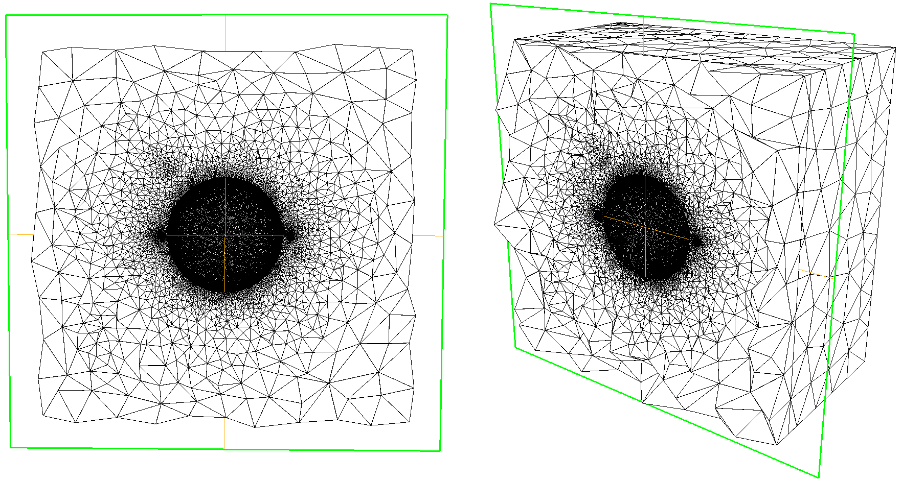
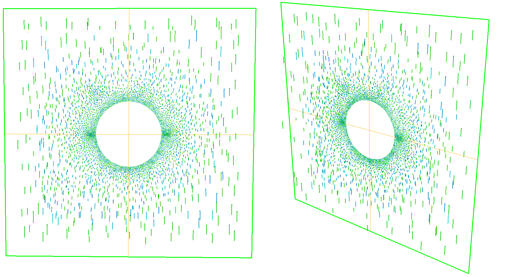
The code has been written and tested first for the case of a spherical colloidal particle of diameter $2R=1\mu m$, posed in the center of a cubic cell with $d=2\mu m$, full of nematic with values of the material constants $L$, $A,B,C$ for the 5CB type (for their values see for ex. [1, 6]). The boundary conditions matched the experimental ones described above. As at some sides the real (experimental) cell is very large (virtually infinite), and full of nematic, an approximation was made in the computations, putting at that sides, i.e., the walls of the computational cell, boundary conditions matching the behaviour of nematic at a longer distance.

All the computations runned on one processor of a 64-bit desktop machine with Intel Core 2Quad CPU Q9550@2.83GHz$\times$4 processor, with 7.7GiB of RAM and the 64-bit Linux Ubuntu 12.04.4 LTS operating system. The FreeFem++ version used was 3.30. The main code in the remeshing process, mmg3d5ljll, for the moment not part of the standard FreeFem++ distribution yet, was cordially supplied by its authors Charles Dapogny, Cécile Dobrzynski, and Pascal Frey, and called as an external module. All runs were reniced at their beginning to a nice value of -10, i.e., to a higher priority.

4.2.1 Main scheme

After being launched, the overall algorithm works in the following way (see Alg. 1, written in pseudo-code, below).

First the initialization of the system is made. The initial mesh Th is built, and the starting guess for Qh set. Then, after the computation of the initial nematic structure into Qh, with Newton iteration (and possibly also steepest descent), the main loop is entered. Here, at each iteration k the current mesh is adapted into a new mesh, and a new nematic structure is computed on it. This is looped for totally NbOfAdapt times, which is a positive integer fixed by the length of the arrays of parameters tolAdapt and errm. Finally, the last computed mesh and nematic configuration on it are returned.

Algorithm 1

// MAIN SCHEME:
Main(Sh, f, tolAdapt, errm)
{
  Initialize(Th, Qh; Sh, f);  // Initialization of Th and Qh.
  NbOfAdapt= length(tolAdapt);    // Total nb of adaptations.

  int k= 0;               // Adaptation index is initialized.
  Qh= Calculate_Nematic_Structure(Th, tolAdapt_k);
  while (++k < NbOfAdapt)  {
     Th= Adapt_Mesh(Th, Qh, errm_k);
     Qh= Calculate_Nematic_Structure(Th, tolAdapt_k);
  }
  return Th, Qh;
}

Figure 3: Zoomed enlargments of the mesh (left) and the corresponding nematic director field (right) from Figs. 1 and 2 (both left) around the (Saturn ring) topological defect. In general, the volume (tetrahedral) mesh is more refined where the Hessian of the solution, or other appropriate functions, is larger (e.g., around the defect), and/or where the domain geometry varies (e.g., near the sphere’s surface).

4.2.2 Initialization: initial mesh and starting guess

The surface mesh describing and enclosing the computational spatial domain was designed within the FreeFem++ built-in functionalities, and then tetrahedrized with TetGen [32] as one of its inner modules. More complicated surface meshes can be generated by Gmsh [33], or other (free) mesh generators, and then imported into FreeFem++.

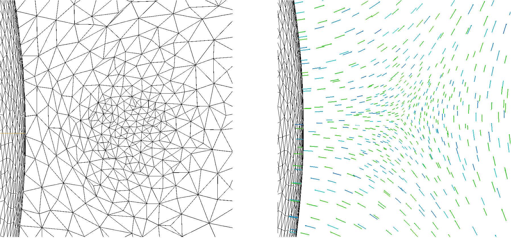
A correct starting guess in this elementary case of a monomer was very simple, i.e., just the constant nematic configuration ${\bf n}=(0,0,1)$. The initial tetrahedral mesh was set fine enough in the neighborhood of the particle, where stronger variations of the nematic field and defects appear, and then linearly coarsened while approaching the cell walls, where the nematic conformation changes no more.

Algorithm 2

// INITIALIZATION:
Initialize(Sh, f, Th, Qh)
{
  Sh= Construct_Surface_Mesh();// Constructs main surface mesh.
  Th= Tetgen(Sh, fine_density);// Fine tetrahedrization.
  f=  Set_Initial_Mesh_Density(Sh);// Sets initial mesh density.
  Th= Tetgen(Sh, f);          // Tetrahedrizes with density f.
  Qh= Set_Starting_Guess(Th); // Starting guess is set.

  return Th, Qh;
}

4.2.3 Newton iteration loop

This is the core, or in any case one of the innest parts of the overall algorithm (the other one is the mesh adaptivity loop). At each step $i$ of the loop, the Newton equation (8) is solved. First the finite element stiffness matrix and load vector are obtained by discretizing the variational equation (8) on the fixed tetrahedral mesh $\mathcal{T}_{k}$, using P1 finite element basis functions. Being the sparse linear system symmetric positive definite, it can thus be solved by the conjugate gradient method (here with an $\varepsilon<0.5\cdot 10^{-7}$ relative error bound, and a rough preconditioner, dividing each line of the sparse matrix with its largest element). This proved to be a good choice in this case, being direct factorization methods, as also GMRES, impracticable, due to the large sizes of the systems. The incremental solution $v^{(i)}$ of the sparse linear system is then added to the current solution $Q^{(i)}$, obtaining $Q^{(i+1)}$, in which the Newton step is again recomputed until the relative change of the functional value (of the system’s free energy) is lower than the tolerance $tol_{k}$, or the maximal number of iterations is reached. In the latter case the algorithm switches into the steepest descent method mood.

Alternatively, the normalized $L_{2}$-norm of the move (increment) $v^{(i)}$ could be used as another (or concurrent) criterion. In our case was anyway being constantly monitored.

4.2.4 Mesh adaptivity loop

Also each mesh adaptation itself is computed iteratively. First a new tetrahedral mesh variable Thx is declared, which is then adapted several times during the loop. Its starting “value” is Th, i.e., the last computed mesh before entering into the mesh adaptivity procedure. Also a set of scalar fields scFields is declared, with regard to which the metrics will be computed.

Once the loop is started, at each new iteration a new finite element space Vhx, based on the current mesh Thx, is declared (which with FreeFem++ is done most easily and straightforwardly with just one short code line). An isotropic metric M is then declared as a scalar field from this FE space, and computed with a call of mshmet. One of the most important parameters of the latter call is errm_k, representing the largest possible relative error of the solution on each element, at the k-th iteration (here ranging within a couple of percents, more precisely starting from 0.02 and ending with 0.01). The other parameter scFields represent the scalar functions with regard to which the metric is computed. Initially these were only the five components $Q_{ij}$ of the tensor order parameter field, and the scalar order parameter $S$ (within the code written as Qh and S). After some experimentations it has been noticed and felt that also the inclusion of the (five) first variations of the free energy $\frac{\delta F}{\delta Q_{ij}}$ could make sense, and so they have been added to the list (as DF).

With this metric M a new mesh is computed into Thx by mmg3d5. The latter takes care that the mesh contains only tetrahedra with side lengths inbetween the (argument) parameters hmin and hmax, and also that the ratio between the side lengths of any two neighbouring tetrahedra does not exceed the prescribed mesh graduality parameter value hgrad, (here fixed to 2.00 throughout all the calculations).

The loop ends when a condition characterizing some kind of convergence of the mesh (and/or the metric) is fullfilled. The condition must measure how much two subsequent meshes are close to each other. What we used here, was very simple, and most probably far from optimal, i.e., we used that the difference of the numbers of the vertices between two subsequent meshes in the loop does not exceed a certain number (here fixed to 300). Alternatively, another condition defined with the norm of the difference between two subsequent metrics could perhaps also be used, and would probably be more recommendable.

In any case, the loop was set to stop at NAdaptIter iterations (here fixed to 20).

Algorithm 3

// MESH ADAPTATION:
Adapt_Mesh(Th, Qh; hmax, errm_k)   // Other possible parameters:
{                                  //  hmin, hgrad (here fixed).
   mesh3 Thx= Th; // Declares and initializes new mesh variable.
   scFields= {Qh, S, DF};  // Scalar fields for metric calculus.

   for (j=1; j<=NAdaptIter; ++j)  {
      fespace Vhx(Thx, P13d);          // Declares new FE space.
      Vhx M= mshmet(Thx, scFields, hmin, hmax, errm_k);//Metric.
      Thx= mmg3d5ljll(Thx, M, hmin, hmax, hgrad);  // Remeshing.
      if (meshes close enough)  break;   // Loop-exit condition.
   }
   return Th=Thx, Qh;
}

5 Numerical results

The present overall scheme is supposed to serve as a case for a wider class of nonlinear calculations. Many other, similar nonlinear problems, perhaps arising from different types of physics, are awaiting to be solved, or the methods for their solution waiting to be improved. A topic in this context that seemed quite important to our perception, and not so much treated until now, is how to drive such a nonlinear algorithm in presence of mesh adaptivity. The latter didn’t appear a so clear task about which it could be straightforwardly possible to make definite statements. But with systematic examination by running many computations, some patterns could be noticed indicating a kind of behaviour.

With the aid of collaborators who further developed the key codes mmg3d5 and mshmet, i.e. their authors, we first made smoothly work the trinom composed by the two and FreeFem++, the latter being the central programming language/software used, strongly FEM-oriented, in which our main code was written. This meant smoothing out their functioning as single entities, as well as their interfacing/communication with FreeFem++.

Plenty of preliminary tests were performed, in total several hundreds, may be thousand, each lasting from several hours to some days, on several cases of nematic colloidal systems. Apart from the monomer one, a lot of trials have been made also for the dimer, or for assemblies of several colloidal particles, i.e., for the so-called colloidal crystals, which could be two- or three-dimensional, as for ex. $2\times 2$, or $2\times$3, or $2\times 2\times 2$, etc.

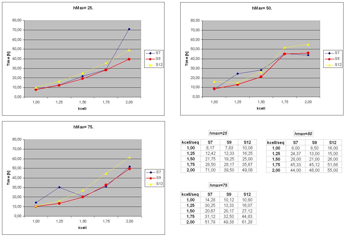
First it was recognized that the computations’ behaviour of nonlinear finite elements based algorithms including mesh adaptivity is in general very parameter-dependent. Changing the value of only one parameter can quite boldly modify the behaviour of entire sets of calculations. This proved in the case of hmax, the parameter representing the maximally allowed length of tetrahedral edges, as it will be possible to notice further ahead, by comparing the computational results/measurements in the tables from Fig. 4.

After these very extensive preliminary tests, and after the above mentioned computational trinom was set and working, we performed three sets of computations on the simplest of nematic colloidal cases, the monomer, for three values of hmax. The latter indicated that the overall loop seems to be driven mostly by two factors.

Mesh	S7		S9		S12
adaptation	tolAdapt	errm	tolAdapt	errm	tolAdapt	errm
$0.$	0.5e-4	0.020	0.5e-4	0.020	0.5e-4	0.020
$1.$	0.5e-3	0.020	0.5e-3	0.020	0.5e-3	0.020
$2.$	0.5e-3	0.015	0.5e-3	0.015	0.5e-3	0.015
$3.$	0.5e-4	0.015	1.0e-4	0.020	1.0e-4	0.020
$4.$	0.5e-5	0.015	1.0e-4	0.015	1.0e-4	0.015
$5.$	0.5e-5	0.010	0.5e-4	0.015	0.5e-4	0.020
$6.$	1.0e-6	0.015	1.0e-5	0.015	0.5e-4	0.015
${\bf 7}.$	1.0e-6	0.010	0.5e-5	0.015	1.0e-5	0.015
$8.$			0.5e-5	0.010	1.0e-5	0.015
${\bf 9}.$			1.0e-6	0.010	0.5e-5	0.015
$10.$					0.5e-5	0.010
$11.$					1.0e-6	0.015
${\bf 12}.$					1.0e-6	0.010

Table 1: Three sequences (arrays) used in calculations.

The first one is when (at what conditions) each new mesh adaptation is triggered. This is determined by the threshold values of the free energy relative variations, and by how are they distributed throughout the nonlinear computation.

The second factor influencing the algorithm’s behaviour resulted to be how the mesh adaptivity is done, i.e., how the new mesh is rebuilt from the previous one at each mesh adaptation. This most strongly depends on the value of the solution error parameter, i.e. errm_k, appearing as argument in mshmet. In fact, the call of the latter constructs the metric with which mmg3d5 then rebuilds the new mesh.

On empirical basis of the hereby presented computations, we argue that a more general algorithm regulating both factors (and possible others, which weren’t explicitly detected yet) should be a loop, or possibly several nested ones, with appropriate stopping conditions. We guess this could guarantee the larger flexibility needed for more general purposes. In fact we recognized (had the confirmation), as said before, that with finite elements based nonlinear algorithms with mesh adaptivity is in general not so easy to predict exactly how a nonlinear computation will behave, thus neither how much it will last before converging.

Thus, to proceed by steps, we confined ourselves to arrange the threshold values in a fixed array we called tolAdapt, its constant length a priori determining how many times the mesh will be adapted, and its entries specifying at what thresholds. We set three such arrays, or sequences (see Table 1), calling them S7, S9, S12 with their integer suffix being their length, and used each of them in a set of computations with varying size of the system, determined by its coefficient kcell.

kcell/seq.	S7	S9	S12
1,00	265285	261669	261552
1,25	348853	346761	342469
1,50	453226	437642	429681
1,75	542873	534595	541236
2,00	653378	625876	621104

Table 2: Numbers of vertices used in calculations for ${\tt hmax}=25$. Numbers for ${\tt hmax}=50$ and $75$ were similar, mostly slightly decreasing for a couple of percents with increasing values of hmax.

Summarizing, what mostly drives the overall nonlinear algorithm is when the mesh adaptivity is triggered, and how the respective new mesh is done. That is, at what free energy thresholds, and within what errors. An empirical proof of the fact, that it is not the same what strategy is brought into play, can be inferred from the tables in Fig. 4 , showing that computations with the sequence S9 were in almost all cases faster of those computed with the other two, S7 and S12, or in the worst case comparable — just slightly slower.

Figure 4: Computation times for values of ${\tt hmax}=25,50,75$. In all three cases the sequence S9 behaves better than the other two (almost everywhere).

Regarding what properties the sequences of free energy threshold and mesh error values must have, it soon appeared quite evident that the values of the tolerances must be decreasing. In fact, at the start of a single simulation run, the initially computed nematic conformations are usually still quite far from the final (equilibrium) solution, i.e., the final nematic structure, and so the mesh adaptations must be more frequent. Here, at each adapted mesh there’s still no real need for convergence to a higher accuracy. So the threshold values at the beginning of any sequence can be larger of those in the proceeding.

Similarly, also the sequence of values of the solution error parameter errm must tend to decrease, altough not necessarily completely monotonically. In reality, they must decrease at each (constant) threshold value.

Moreover, the present case suggested that the sequence of thresholds should be of intermediate length, as for ex. S9, i.e., neither too long, like S12, nor too short, like S7.

Therefore, since typologies of physical systems and their sizes vary in general, and the parameter sequences should in general vary with them too, in both length and values composition, it seemingly should make sense that the use of sequences in fixed arrays could, as mentioned earlier, be changed in the future by the use of one or more loops, possibly nested, satisfying suitable stopping conditions, that could drive the mesh adaptivity process optimally, or nearly so.

6 Conclusions and suggestions for the future

In this work a numerical method for functional minimization of tensor fields on bounded, simply connected domains of Euclidean space $\mathbb{R}^{3}$ has been developed on the Landau-de Gennes case describing confined nematic colloidal systems. Altough similar codes already exist, this finite elements based algorithm for the first time employs a systemic mesh adaptivity approach in 3D, with use of metrics (isotropic case).

Anyhow, coupling the mesh adaptation process with the nonlinear scheme shows a strong parametric dependence. For the time being we solved it by a priori setting sequences of the driving parameters into fixed arrays. Computations made for three different sequences, which were also of different length, empirically demonstrated the parametric dependence and gave some insight into the process behaviour.

For a more general solution of this mesh adaptivity-driving task, that would be appropriate for a more ample class of nematic colloidal systems and other kind of physics problems, possibly dynamical, we imagine and would like to advocate the introduction of a special auxiliary algorithm, using for ex. several nested while-loops, which would be flexible enough for such purposes.

When this and perhaps some other, more technical, questions will be optimized, the here presented methodology could be assumed to be ready for more intensive calculations, aimed at systematic research in theoretical pyhsics.

Extensions of the presented methodology could be envisaged also in directions of solving PDEs on more general manifolds[35], and/or the possible introduction of geometric integration [36] for dynamical problems.

7 Appendix

7.1 First and second variation of $F$

To implement equation (8) into our code following [25], the first and second variation of the free energy functional $F$ need to be calculated. We compute them analytically, the first one for both Newton iteration and steepest descent, and the second one just for Newton.

Before that, we must first of all solve the task of preserving the traceless and simmetricity conditions of $Q$. This could have perhaps been done by the introduction of a special symmetric and traceless tensorial basis [37], which by construction preserves both conditions, as done for ex. in [9]. Alternatively, we have opted to just apply the substitutions $Q_{33}=-Q_{11}-Q_{22}$ and $Q_{j\,i}=Q_{ij}$ into the free energy expressions, after which the forms of the free energy densities $f_{e}$, $f_{b}$ and $f_{s}$ depend only on the five components $Q_{11}$, $Q_{22}$, $Q_{12}$, $Q_{13}$, $Q_{23}$. All the following calculations have then been derived by taking into account only these components. So the elastic free energy density becomes

$$f_{e}(\nabla Q)=L\left(\nabla Q_{ij}\cdot\nabla Q_{ij}+\nabla Q_{11}\cdot\nabla Q_{22}\right),$$ (12)

and the surface energy density

$$f_{s}(Q)=W\left[(Q_{ij}-Q_{ij}^{0})(Q_{ij}-Q_{ij}^{0})+(Q_{11}-Q_{11}^{0})(Q_{22}-Q_{22}^{0})\right].$$ (13)

After some symbolic computer calculations, omitted here for brevity, also $f_{b}$ has been transformed by substitutions into a polynomial of 4th degree in the actual five components $Q_{ij}$.

Without digging too deeply into formalism, we will just assume that the previous notation for the tensor field $Q$ will from now on mean the five-tuple $Q=(Q_{11},Q_{22}$, $Q_{12}$, $Q_{13}$, $Q_{23})$, and similarly for all the other tensor field quantities, as $\delta Q$, $\varphi$, and $v$. For a formally exhaustive and more abstract treatment in a Sobolev space setting, the reader is referred to [8].

The first variation of the Landau-de Gennes free energy $F$ (4) is

$$\delta F(Q)=F^{\prime}(Q)\phi=\int_{\Omega}\left[\frac{\partial f_{e}}{\partial\nabla Q_{ij}}\cdot\nabla\phi_{ij}+\frac{\partial f_{b}}{\partial Q_{ij}}\phi_{ij}\right]dV+\int_{\Gamma_{p}}\frac{\partial f_{s}}{\partial Q_{ij}}\,\phi_{ij}~{}dA,$$ (14)

where instead of $\delta Q_{ij}$ we already introduced the notation $\phi_{ij}$ for the test functions, having well in mind that the pairs of indexes $ij$ have only the five couples of values defined above. Variating again leads us to the second variation

$$\delta^{2}F(Q)=F^{\prime\prime}(Q)\phi v=\int_{\Omega}\left[\frac{\partial}{\partial\nabla Q_{kl}}\left(\frac{\partial f_{e}}{\partial\nabla Q_{ij}}\cdot\nabla\phi_{ij}\right)\cdot\nabla v_{kl}+\frac{\partial}{\partial Q_{kl}}\left(\frac{\partial f_{b}}{\partial Q_{ij}}\phi_{ij}\right)v_{kl}\right]dV$$

$$+\int_{\Gamma_{p}}\frac{\partial}{\partial Q_{kl}}\left(\frac{\partial f_{s}}{\partial Q_{ij}}\phi_{ij}\right)v_{kl}~{}dA~{}.$$ (15)

The terms of the first variation for the elastic part are now easily obtained as

$$\frac{\partial f_{e}}{\partial\nabla Q_{ij}}\cdot\nabla\phi_{ij}=2L\left[\nabla Q_{ij}\cdot\nabla\phi_{ij}+\frac{1}{2}(\nabla Q_{22}\cdot\nabla\phi_{11}+\nabla Q_{11}\cdot\nabla\phi_{22})\right],$$

as also those for the second variation,

$$\frac{\partial}{\partial\nabla Q_{kl}}\left(\frac{\partial f_{e}}{\partial\nabla Q_{ij}}\cdot\nabla\phi_{ij}\right)\cdot\nabla v_{kl}=2L\left[\nabla v_{ij}\cdot\nabla\phi_{ij}+\frac{1}{2}(\nabla v_{22}\cdot\nabla\phi_{11}+\nabla v_{11}\cdot\nabla\phi_{22})\right],$$

where perhaps worth to be noted is the appearence of mixed terms. Similarly, the surface terms for the first variation are

$$\frac{\partial f_{s}}{\partial Q_{ij}}\phi_{ij}=2W\left[(Q_{ij}-Q_{ij}^{0})\phi_{ij}+\frac{1}{2}\left((Q_{22}-Q_{22}^{0})\phi_{11}+(Q_{11}-Q_{11}^{0})\phi_{22}\right)\right],$$

while those for the second read

$$\frac{\partial}{\partial Q_{kl}}\left(\frac{\partial f_{s}}{\partial Q_{ij}}\phi_{ij}\right)v_{kl}=2W\left[v_{ij}\phi_{ij}+\frac{1}{2}(v_{22}\phi_{11}+v_{11}\phi_{22})\right],$$

where again similar mixed terms appear. The concrete calculations for both variations of the concrete $f_{b}(Q)$ has been done with the help of the symbolic software Mathematica.

7.2 Steepest descent

7.2.1 Gradient calculation

The gradient, that we usually denote by $h$ (here with $h=-\nabla F(Q)$, following the notation of Polak [26]), is an element of the Hilbert space, in which we are seeking the solution $Q^{*}$. For its calculation we use the Riesz theorem from basic functional analysis, which states that for each linear continuous functional $G$, mapping from a Hilbert space $\mathcal{H}$ into $\mathbb{R}$, there exists exactly one element $h\in\mathcal{H}$, such that the functional values $G(Q)$ is equal to the scalar product $<Q,\,h>$ for each element $Q$ from $\mathcal{H}$.

In our case the functional $G$ is the differential of the free energy functional $F$ in a configuration $Q$, i.e., $DF(Q)$. Denoting now the gradient by $h$, and expanding it as $h=\sum_{i=1}^{N}h_{i}\phi_{i}$, i.e., by the basis functions of the Hilbert space $\mathcal{H}$ to which it belongs, we obtain

$$<Q,h>=\sum_{j=1}^{N}h_{j}<Q,\phi_{j}>.$$ (16)

As we want this to hold for every $Q$, we set $Q=\phi_{i}$, for each $i$, getting

$$<\phi_{i},h>=\sum_{j=1}^{N}h_{j}<\phi_{i},\phi_{j}>,~{}~{}~{}i=1,\dots,N.$$ (17)

Being $<\phi_{i},h>$ equal to the $i$-th gradient coefficient $h_{i}$, and $<\phi_{i},\phi_{j}>$ to the $ij$-th element of the Gram matrix, the calculation of the Hilbert space gradient is accomplished by first computing the Gram matrix $K$, thus all the possible scalar products between the basis functions $\phi_{i}$, that is $K_{ij}\,=\,<\phi_{\,i},\phi_{j}>$ (here we note that the Gram matrix is sparse). Besides, the negative of the differential (i.e. first variation) of $F$ is evaluated in the momentary configuration $Q$, obtaining the right-hand side $d=\{-DF(Q)(\phi_{i})\}_{i=1}^{N}$ of the linear system $Kh=d$. By solving it,  we obtain the gradient $h=\{-\nabla F(Q)(\phi_{i})\}_{i=1}^{N}$.

7.2.2 Scalar product choice

To implement this procedure, a choice of the scalar product must be made. Following the structure of the Landau-de Gennes free energy, we define, similarly as in [3], the scalar product as

$$<Q,P>:=\int_{\Omega}\frac{1}{2}\,L\,\nabla Q_{ij}\cdot\nabla P_{j\,i}+\frac{1}{2}\,A\,Q_{ij}P_{j\,i}\,dV+\int_{\partial\Omega}\frac{1}{2}WQ_{ij}\,P_{j\,i}\,dA,$$ (18)

where Einstein summation is here for now employed over all the indexes $i,j=1,2,3$. The constant term $Q^{0}$ under the surface integral has been dropped to preserve the definition scalar product property of $<Q,\,Q>$ vanishing only for $Q=0$, and the constants left to mantain appropriate proportions between the addends.

After applying the traceless condition $Q_{33}=-Q_{11}-Q_{22}$, and symmetricity $Q_{ij}=Q_{j\,i}$, we obtained

$$<Q,P> = \int_{\Omega}L\,(\nabla Q_{ij}\cdot\nabla P_{ij}+\frac{1}{2}\,(\nabla Q_{11}\cdot\nabla P_{22}+\nabla Q_{22}\cdot\nabla P_{11}))$$ (19)

$$+ A\,(Q_{ij}P_{ij}+\frac{1}{2}\,(Q_{11}P_{22}+Q_{22}P_{11}))\,dV$$

$$+ \int_{\partial\Omega}W(Q_{ij}\,P_{ij}+\frac{1}{2}\,(Q_{11}P_{22}+Q_{22}P_{11}))\,dA$$

where, among the Einstein summation through only five index pairs, additional mixed terms in the index pairs 11 and 22 appear. For exactly traceless (and symmetric) tensor fields this is a scalar product. But for tensor fields which are numerically non-exactly traceless, it is no longer such, lacking again the property that $<Q,Q>$ has to vanish only when $Q=0$. Thus, after some experiments the mixed terms has been dropped, finally leaving

$$<Q,P> = \int_{\Omega}\left(L\,\nabla Q_{ij}\cdot\nabla P_{ij}+|A|\,Q_{ij}P_{ij}\right)\,dV+\int_{\partial\Omega}WQ_{ij}\,P_{ij}\,dA,$$ (20)

where the absolute value brackets has been added to the constant $A$, otherwise the product could sometimes be negative, and thus obviously contraddicting the nonnegativity condition of the scalar product.

7.2.3 Exact line search

At each steepest descent iteration the calculated gradient gives only the direction of the maximal descent, but lets unsolved how much one should move in this direction. Thus, the iteration step must include also the choice of a proper coefficient $\lambda\geq 0$. This can be crucial for the convergence itself, as for the time dependence of the iteration. The optimal choice for $\lambda$ is the solution of the minimization problem

$$\lambda^{*}=\arg\min_{\lambda}\{F(Q+\lambda h)\},$$ (21)

which is called exact line search. This can seldom be too expensive, thus leading to a preference for approximative methods as for example the Armijo method [26]. But in the present case it leads to a not too complex or expensive situation. For the Landau-de Gennes functional the problem (21) means

$$F(Q+\lambda h) = \int_{\Omega}\left[f_{e}(\nabla Q+\lambda\nabla h)+f_{b}(Q+\lambda h)\right]dV+\int_{\Gamma_{p}}f_{s}(Q+\lambda h)dA,$$ (22)

which can be quite easily expanded and collected with regard to powers of $\lambda$, here done once with Mathematica, and then transcribed into the FreeFem++ code. After obtaining the coefficient terms by integration (here done within the code), one in fact gets a polynomial of fourth order in dependence of $\lambda$:

$$p(\lambda)=a_{0}+a_{1}\lambda+a_{2}\lambda^{2}+a_{3}\lambda^{3}+a_{4}\lambda^{4}.$$

Extremal values are found when $p^{\prime}(\lambda)=0$, that is, when

$$p^{\prime}(\lambda)=a_{1}+2a_{2}\lambda+3a_{3}\lambda^{2}+4a_{4}\lambda^{3}=0,$$

the three zeros of which are found with a GSL numerical procedure [34]. The minimal root between them is taken as the optimal $\lambda^{*}$, after a verification of the positiveness of $p^{\prime\prime}$ in it as the minimum condition. During concrete computations $\lambda^{*}$ usually ranged around values between 0.01 and 0.3, while the other two roots were almost always pairs of complex conjugated zeros, thus not feasible candidates.

Acknowledgments. Miha Ravnik, Daniel Svenšek, and George Mejak (University of Ljubljana) are acknowledged for useful discussions, and Pierre-Henri Tournier (UPMC, Paris) for help with debugging of the FreeFem++ related internal and external modules.

References

- [1] I. Muševič, M. Škarabot, U. Tkalec, M. Ravnik and S. Žumer, Two-dimensional nematic colloidal crystals self-assembled by topological defects. Science (2006), 313, 954.
- [2] P. G. de Gennes and J. Prost, The Physics of Liquid Crystals. Clarendon Press, Oxford, 1993.
- [3] I. Danaila and F. Hecht, A finite element method with mesh adaptivity for computing vortex states in fast-rotating Bose-Einstein condensates. Jour. Comp. Phys. 229 (2010) 6946-6960.
- [4] P. G. de Gennes, Superconductivity in Metals and Alloys. Benjamin, New York, 1966.
- [5] O. Pironneau, Finite Element Methods for Fluids. Wiley, 1989.
- [6] M. Ravnik, M. Škarabot, S. Žumer, U. Tkalec, I. Poberaj, D. Babič, N. Osterman, and I. Musěvič, Entangled Nematic Colloidal Dimers and Wires, Phys. Rev. Lett. 99, 247801 (2007).
- [7] M. Škarabot, M. Ravnik, S. Žumer, U. Tkalec, I. Poberaj, D. Babič, N. Osterman and I. Muševič, Two-dimensional dipolar nematic colloidal crystals. Phys. Rev. E 76, 051406 (2007).
- [8] T. A. Davis and E. C. Gartland, Jr, Finite element analysis of the Landau-de Gennes minimization problem for liquid crystals. SIAM J. Numer. Anal. 35, 336-362 (1998).
- [9] R. James, E. Willman, F. A. Fernández and S. E. Day, Finite-element modeling of liquid-crystal hydrodynamics with a variable degree of order. IEEE Transactions on Electron Devices Vol. 53, No. 7, July 2006.
- [10] S. R. Seyednejad, M. R. Mozaffari and M. R. Ejtehadi, Confined nematic liquid crystal between two spherical boundaries with planar anchoring. Phys. Rev. E 88, 012508 (2013).
- [11] R. James, E. Willman, F. A. Fernández, S. E. Day, Computer Modeling of Liquid Crystal Hydrodynamics. IEEE Transactions on Magnetics, Vol. 44, No. 6, pp. 814-817, 2008.
- [12] J. Fukuda, M. Yoneya and H. Yokoyama, Defect structure of a nematic liquid crystal around a spherical particle: adaptive mesh refinement approach, Phys. Rev. E 65, 041709 (2002).
- [13] D. Svenšek, S. Žumer, Backflow-affected relaxation in nematic liquid crystals. Liq. Cryst. 28, 1389 (2001).
- [14] A. de Lózar, W. Schöpf, I. Rehberg, D. Svenšek, L. Kramer, Transformation from walls to disclination lines: Statics and dynamics of the pincement transition. Phys. Rev. E 72, 051713 (2005).
- [15] M. Ravnik and S. Žumer, Nematic colloids entangled by topological defects. S. Matt. Vol. 5, n. 2, 2009, pp. 253–480.
- [16] P. G. Ciarlet, The Finite Element Method for Elliptic Problems. North Holland, New York, 1978.
- [17] F. Hecht and R. Kuate, An approximation of anisotropic metrics from higher order interpolation error for triangular mesh adaptation. Jour. of Comp. and Appl. Math. 258 (2014), pp. 99 115.
- [18] F. Hecht, New development in FreeFem++. J. Numer. Math. 20 (2012), no. 3-4.
- [19] L. D. Landau, Ž. Eksp. Teor. Fiz. 7, pp. 19 32 (1937).
- [20] P. M. Chaikin and T. C. Lubensky, Principles of Condensed Matter Physics. Cambridge University Press, Cambridge, New York, 1997.
- [21] Q. Du, M. D. Gunzburger and J. S. Peterson, Analysis and approximation of the Ginzburg-Landau model of superconductivity. SIAM Review (1992) 34, 1, pp. 54-81.
- [22] P. Ziherl and S. Žumer , Fluctuations of confined liquid crystals above nematic-isotropic phase transition temperature. Phys. Rev. Lett., Vol. 78, n. 4, 27 Jan., 1997.
- [23] I. M. Gelfand and S. V. Fomin, Calculus of Variations. Prentice-Hall, Englewood Cliffs, N. J., 1963.
- [24] W. C. Rheinboldt, Methods for Solving Systems of Nonlinear Equations, 2nd ed. CBMS-NSF Regional Conference Series in Applied Mathematics, Vol. 70 (SIAM, Philadelphia, 1998).
- [25] G. E. Fasshauer, E. C. Gartland, Jr, J. W. Jerome, Newton iteration for partial differential equations and the approximation of the identity. Numerical Algorithms 25, (2000), 181-195.
- [26] E. Polak, Optimization, Algorithms and Consistent Approximations. Springer-Verlag, New York, 1998.
- [27] P. J. Frey, P.-L. George, Mesh Generation. Application to Finite Elements, Second Edition. Wiley, London, 2008.
- [28] F. Alauzet, P. J. Frey, P. L. George and B. Mohammadi, 3D transient fixed point mesh adaptation for time dependent problems. Application to CFD simulations. J. Comp. Phys., Vol. 222, pp. 592-623, 2007.
- [29] Ch. Dapogny, C. Dobrzynski, P. Frey, Three-dimensional adaptive domain remeshing, implicit domain meshing, and applications to free and moving boundary problems. J. Comp. Phys., 262, pp. 358-378, 2014.
- [30] F. Alauzet, Adaptation de maillage anisotrope en trois dimensions. Application aux simulations instationnaires en Mécanique de Fluides. Phd Thesis, Université de Montpellier II, (2003).
- [31] C. Dobrzynski, Adaptation de Maillage anisotrope 3D et application à l’aéro-thermique des bâtiments. Phd Thesis, Université Pierre et Marie Curie, Paris VI (2005).
- [32] Hang Si, TetGen, a quality tetrahedral mesh generator and a 3D Delaunay triangulator. http://tetgen.berlios.de/.
- [33] C. Geuzaine, J.-F. Remacle, Gmsh: a three-dimensional finite element mesh generator with built-in pre- and post-processing facilities. Int. Jour. for Numer. Methods in Engin. 79(11), pp. 1309-1331, 2009.
- [34] GNU Scientific Library, http://www.gnu.org/software/gsl/.
- [35] C. J. Budd, A. Iserles, Geometric integration: Numerical solution of differential equations on manifolds. Phil. Trans. R. Soc. Lond. A, Vol. 357, No. 1754, p. 945-956, 15 April 1999.
- [36] E. Hairer, C. Lubich, G. Wanner, Geometric Numerical Integration: Structure-Preserving Algorithms for Ordinary Differential Equations, 2nd ed. Springer, Berlin, Heidelberg, 2006.
- [37] A. Sonnet, A. Kilian, S. Hess, Alignment tensor versus director: Description of defects in nematic liquid crystals. Phys. Rev. E Vol. 52, N. 1, July, 1995.