EUROPEAN ORGANIZATION FOR NUCLEAR RESEARCH (CERN)

​​​ CERN-PH-EP-2015-127 LHCb-PAPER-2015-020 May 26, 2015

Study of ${{{B}^{-}}}\rightarrow D{{K}^{-}}{{\pi}^{+}}{{\pi}^{-}}$ and ${{{B}^{-}}}\rightarrow D{{\pi}^{-}}{{\pi}^{+}}{{\pi}^{-}}$ decays and determination of the CKM angle $\gamma$

The LHCb collaboration

We report a study of the suppressed ${{{B}^{-}}}\rightarrow D{{K}^{-}}{{\pi}^{+}}{{\pi}^{-}}$ and favored ${{{B}^{-}}}\rightarrow D{{\pi}^{-}}{{\pi}^{+}}{{\pi}^{-}}$ decays, where the neutral $D$ meson is detected through its decays to the $K^{\mp}\pi^{\pm}$ and $C\!P$-even ${{K}^{+}}{{K}^{-}}$ and ${{\pi}^{+}}{{\pi}^{-}}$ final states. The measurement is carried out using a proton-proton collision data sample collected by the LHCb experiment, corresponding to an integrated luminosity of 3.0$\mbox{\,fb}^{-1}$. We observe the first significant signals in the $C\!P$-even final states of the $D$ meson for both the suppressed ${{{B}^{-}}}\rightarrow D{{K}^{-}}{{\pi}^{+}}{{\pi}^{-}}$ and favored ${{{B}^{-}}}\rightarrow D{{\pi}^{-}}{{\pi}^{+}}{{\pi}^{-}}$ modes, as well as in the doubly Cabibbo-suppressed $D\rightarrow{{K}^{+}}{{\pi}^{-}}$ final state of the ${{{B}^{-}}}\rightarrow D{{\pi}^{-}}{{\pi}^{+}}{{\pi}^{-}}$ decay. Evidence for the ADS suppressed decay ${{{B}^{-}}}\rightarrow D{{K}^{-}}{{\pi}^{+}}{{\pi}^{-}}$, with $D\rightarrow{{K}^{+}}{{\pi}^{-}}$, is also presented. From the observed yields in the ${{{B}^{-}}}\rightarrow D{{K}^{-}}{{\pi}^{+}}{{\pi}^{-}}$, ${{{B}^{-}}}\rightarrow D{{\pi}^{-}}{{\pi}^{+}}{{\pi}^{-}}$ and their charge conjugate decay modes, the most probably value of the weak phase $\gamma$ corresponds to $\gamma=(74^{+20}_{-19})^{\rm o}$. This is one of the most precise single-measurement determinations of $\gamma$ to date.

Published in Phys. Rev. D

© CERN on behalf of the LHCb collaboration, licence CC-BY-4.0.

 

1 Introduction

The study of beauty and charm hadron decays provides a powerful probe to search for physics beyond the Standard Model that is complementary to direct searches for new, high-mass particles. In the Standard Model, the flavor-changing charged currents of quarks are described by the 3$\times$3 unitary complex-valued Cabibbo-Kobayashi-Maskawa (CKM) mixing matrix [1, 2], whose elements, $V_{\ij}$ ($i=u,c,t$ and $j=d,s,b$), quantify the relative $i\leftrightarrow j$ coupling strength. Its nine matrix elements can be expressed in terms of four independent parameters, which need to be experimentally determined.

In general, decay rates that involve the $i\leftrightarrow j$ quark transition are sensitive to the magnitudes of the CKM matrix elements, $|V_{ij}|$. The (weak) phases between different CKM matrix elements can be probed by studying the interference between two (or more) decay amplitudes. Particle and antiparticle amplitudes are related by the $C\!P$ operator, where $C$ signifies charge conjugation, and $P$ refers to the parity operator. Under the $C\!P$ operation, weak phases flip sign, leading to different decay rates for particles and antiparticles, if the weak and ($C\!P$-invariant) strong phases differ between the contributing amplitudes. Precision measurements of the magnitudes and phases of the CKM elements provide constraints on many possible scenarios for physics beyond the Standard Model.

One of the least well-measured phases is $\gamma\equiv\text{arg}[-(V_{ud}V^{*}_{ub})/(V_{cd}V^{*}_{cb})]$, which can be probed by studying the interference between $b\rightarrow u$ and $b\rightarrow c$ transitions. The most promising method to determine $\gamma$ is to study the interference between ${{{B}^{-}}}\rightarrow{{D}^{0}}{{K}^{-}}$ and ${{{B}^{-}}}\rightarrow{{\kern 1.99997pt\overline{\kern-1.99997ptD}{}}{}^{0}}{{K}^{-}}$ decays, when states accessible to both the ${{D}^{0}}$ and ${{\kern 1.99997pt\overline{\kern-1.99997ptD}{}}{}^{0}}$ mesons are selected. These modes are particularly attractive for the determination of $\gamma$ because their amplitudes are dominated by only a pair of tree-level processes, leading to a small theoretical uncertainty [3]. Hereafter, we use $D$ without a charge designation when the charm meson can be either a ${{D}^{0}}$ or ${{\kern 1.99997pt\overline{\kern-1.99997ptD}{}}{}^{0}}$. A number of methods, depending on the $D$ decay mode, have been discussed in the literature, and are often grouped into three categories: (i) $C\!P$ eigenstates, such as $D\rightarrow{{K}^{+}}{{K}^{-}}$ and $D\rightarrow{{\pi}^{+}}{{\pi}^{-}}$ decays [4, 5] (GLW); (ii) flavor-specific final states, such as the Cabibbo-favored (CF) and doubly Cabibbo suppressed (DCS) $D\rightarrow K^{\pm}\pi^{\mp}$ decays [6, 7] (ADS); and (iii) multi-body self-conjugate final states, such as $D\rightarrow{{K}^{0}_{\rm\scriptscriptstyle S}}{{\pi}^{+}}{{\pi}^{-}}$ [8] (GGSZ).

Beyond this simplest set of modes, these techniques are also applicable to modes with vector mesons, such as ${{{B}^{-}}}\rightarrow{D}^{*}{{K}^{-}}$, ${{\kern 1.79993pt\overline{\kern-1.79993ptB}{}}{}^{0}}\rightarrow D{{\kern 1.99997pt\overline{\kern-1.99997ptK}{}}{}^{*0}}$ [9], and ${{B}^{0}_{s}}\rightarrow D\phi$ [5], as well as $b$-baryon decays, e.g. ${{\mathchar 28931\relax}^{0}_{b}}\rightarrow D{\mathchar 28931\relax}$ [10, 11, 12] decays. It has also been suggested that other multi-body final states of the recoiling strange quark system could be useful [13], due to the larger branching fractions to these final states, and potentially a larger interference contribution.

The current experimental measurements, averaged over several decays modes, are $\gamma=(73^{+9}_{-10})^{\rm o}$ by the LHCb collaboration [14, *LHCb-CONF-2014-004], $\gamma=(69^{+17}_{-16})^{\rm o}$ by the BaBar collaboration [16], and $\gamma=(68^{+15}_{-14})^{\rm o}$ by the Belle collaboration [17]. The overall precision on $\gamma$ from a global fit to direct measurements of $\gamma$ is about $7^{\rm o}$ [18]. To improve the overall precision on $\gamma$, it is important to study a wide range of final states.

In this article, we present the first ADS and GLW analyses of the decay ${{{B}^{-}}}\rightarrow DX_{s}^{-}$, where the $D$ meson is observed through its decay to $K^{\pm}\pi^{\mp}$, ${{K}^{+}}{{K}^{-}}$ and ${{\pi}^{+}}{{\pi}^{-}}$ final states and $X_{s}^{-}\equiv{{K}^{-}}{{\pi}^{+}}{{\pi}^{-}}$. When specific charges are indicated in a decay, charge conjugation is implicitly included, except in the definition of asymmetries discussed below. The measurements use proton-proton ($pp$) collision data collected by the LHCb experiment, corresponding to an integrated luminosity of 3.0$\mbox{\,fb}^{-1}$, of which 1.0$\mbox{\,fb}^{-1}$ was recorded at a center-of-mass energy of 7$\mathrm{\,Te\kern-1.00006ptV}$ and 2.0$\mbox{\,fb}^{-1}$ at 8$\mathrm{\,Te\kern-1.00006ptV}$.

2 Formalism

The formalism that was developed to describe the ${{{B}^{-}}}\rightarrow D{{K}^{-}}$ modes can be applied in the ${{{B}^{-}}}\rightarrow DX_{s}^{-}$ case with only minor modifications [13]. The decay rates in the $C\!P$ final states can be expressed as

$$\Gamma({{{B}^{-}}}\rightarrow[h^{-}h^{+}]_{D}X_{s}^{-}) \propto 1+r_{B}^{2}+2\kappa r_{B}\cos(\delta_{B}-\gamma),$$ (1)

$$\Gamma({{{B}^{+}}}\rightarrow[h^{-}h^{+}]_{D}X_{s}^{+}) \propto 1+r_{B}^{2}+2\kappa r_{B}\cos(\delta_{B}+\gamma).$$ (2)

Here, $h^{\pm}=\pi^{\pm}$ or $K^{\pm}$, and $[h^{-}h^{+}]_{D}$ indicates that the state in brackets is produced in the decay of the neutral $D$ meson. The quantities $r_{B}\equiv|A({{{B}^{-}}}\rightarrow[h^{-}h^{+}]_{{{\kern 1.39998pt\overline{\kern-1.39998ptD}{}}{}^{0}}}X_{s}^{-})/A({{{B}^{-}}}\rightarrow[h^{-}h^{+}]_{{{D}^{0}}}X_{s}^{-})|$ and $\delta_{B}$ are the amplitude ratio and strong phase difference between ${{{B}^{-}}}\rightarrow{{\kern 1.99997pt\overline{\kern-1.99997ptD}{}}{}^{0}}X_{s}^{-}$ and ${{{B}^{-}}}\rightarrow{{D}^{0}}X_{s}^{-}$ contributions, averaged over the $DX_{s}^{-}$ phase space. The parameter $\kappa$ is a coherence factor that accounts for a dilution of the interference due to the variation of the strong phase across the phase space; its value is bounded between 0 and 1. In principle, $\kappa$ can be obtained in a model-dependent way by a full amplitude analysis of this decay. Here, we consider it as a free parameter to be determined in the global fit for $\gamma$. The strong parameters, $r_{B}$, $\delta_{B}$ and $\kappa$ are specific to this decay, and differ from those obtained from other $B\rightarrow DK$ modes.

The decay rates for the $D\rightarrow K^{\pm}\pi^{\mp}$ final states can be written as

$$\Gamma({{{B}^{-}}}\rightarrow[{{K}^{+}}{{\pi}^{-}}]_{D}X_{s}^{-}) \propto r_{B}^{2}+r_{D}^{2}+2\kappa r_{B}r_{D}\cos(\delta_{B}+\delta_{D}-\gamma),$$ (3)

$$\Gamma({{{B}^{+}}}\rightarrow[{{K}^{-}}{{\pi}^{+}}]_{D}X_{s}^{+}) \propto r_{B}^{2}+r_{D}^{2}+2\kappa r_{B}r_{D}\cos(\delta_{B}+\delta_{D}+\gamma),$$ (4)

$$\Gamma({{{B}^{-}}}\rightarrow[{{K}^{-}}{{\pi}^{+}}]_{D}X_{s}^{-}) \propto 1+(r_{B}r_{D})^{2}+2\kappa r_{B}r_{D}\cos(\delta_{B}-\delta_{D}-\gamma),$$ (5)

$$\Gamma({{{B}^{+}}}\rightarrow[{{K}^{+}}{{\pi}^{-}}]_{D}X_{s}^{+}) \propto 1+(r_{B}r_{D})^{2}+2\kappa r_{B}r_{D}\cos(\delta_{B}-\delta_{D}+\gamma).$$ (6)

Here, additional parameters $r_{D}$ and $\delta_{D}$ enter, which quantify the ratio of the DCS to CF amplitude, $A({{D}^{0}}\rightarrow{{K}^{+}}{{\pi}^{-}})/A({{D}^{0}}\rightarrow{{K}^{-}}{{\pi}^{+}})=r_{D}e^{i\delta_{D}}$. Values of $r_{D}$ and $\delta_{D}$ are taken from independent measurements [19, 20].

The determination of the $C\!P$ observables in the ${{{B}^{-}}}\rightarrow DX_{s}^{-}$ decay uses the favored ${{{B}^{-}}}\rightarrow D{{\pi}^{-}}{{\pi}^{+}}{{\pi}^{-}}$ decay for normalization, denoted here as ${{{B}^{-}}}\rightarrow DX_{d}^{-}$. For brevity, we will use $X^{-}$ to refer to either $X_{d}^{-}$ or $X_{s}^{-}$. In addition, $D\rightarrow K\pi$ is used when both charge combinations are considered.

The $C\!P$ observables of interest for the GLW analysis are the charge-averaged yield ratios

$$R^{h^{+}h^{-}}_{{C\!P}+} \equiv 2\frac{\Gamma({{{B}^{-}}}\rightarrow[h^{+}h^{-}]_{D}X_{s}^{-})+\Gamma({{{B}^{+}}}\rightarrow[h^{+}h^{-}]_{D}X_{s}^{+})}{\Gamma({{{B}^{-}}}\rightarrow[{{K}^{-}}{{\pi}^{+}}]_{D}X_{s}^{-})+\Gamma({{{B}^{+}}}\rightarrow[{{K}^{+}}{{\pi}^{-}}]_{D}X_{s}^{+})}$$

$$=1+r_{B}^{2}+2\kappa r_{B}\cos\delta_{B}\cos\gamma.$$ (7)

Because of the different $D$ final states in Eq. 7, systematic uncertainty due to the precision of the $D$ branching fractions and the different selections is incurred. Following Ref. [13], we neglect $C\!P$ violation in the ${{{B}^{-}}}\rightarrow DX_{d}^{-}$ and the favored $D$ final state of ${{{B}^{-}}}\rightarrow DX_{s}^{-}$ decays, and approximate $R^{h^{+}h^{-}}_{{C\!P}+}$ by the following double ratio

$$R_{{C\!P}+}\simeq\frac{R^{h^{+}h^{-}}_{s/d}}{R^{K\pi}_{s/d}},$$ (8)

where

$$R^{h^{+}h^{-}}_{s/d} \equiv\frac{\Gamma({{{B}^{-}}}\rightarrow[h^{+}h^{-}]_{D}X_{s}^{-})+\Gamma({{{B}^{+}}}\rightarrow[h^{+}h^{-}]_{D}X_{s}^{+})}{\Gamma({{{B}^{-}}}\rightarrow[h^{+}h^{-}]_{D}X_{d}^{-})+\Gamma({{{B}^{+}}}\rightarrow[h^{+}h^{-}]_{D}X_{d}^{+})},$$ (9)

$$R^{K\pi}_{s/d} \equiv\frac{\Gamma({{{B}^{-}}}\rightarrow[{{K}^{-}}{{\pi}^{+}}]_{D}X_{s}^{-}+\Gamma({{{B}^{+}}}\rightarrow[{{K}^{+}}{{\pi}^{-}}]_{D}X_{s}^{+})}{\Gamma({{{B}^{-}}}\rightarrow[{{K}^{-}}{{\pi}^{+}}]_{D}X_{d}^{-}+\Gamma({{{B}^{+}}}\rightarrow[{{K}^{+}}{{\pi}^{-}}]_{D}X_{d}^{+})}.$$ (10)

This double ratio has the benefit that almost all systematic uncertainties cancel to first order. The neglected $C\!P$-violating contribution of magnitude $\kappa r_{B}|{V_{{u}{s}}}{V_{{c}{d}}}/{V_{{u}{d}}}{V_{{c}{s}}}|\lesssim 0.01$ is included as a source of systematic uncertainty.

We also make use of the charge asymmetries

$${\mathcal{A}}^{f}_{X^{\pm}}\equiv\frac{\Gamma({{{B}^{-}}}\rightarrow f_{D}X^{-})-\Gamma({{{B}^{+}}}\rightarrow\bar{f}_{D}X^{+})}{\Gamma({{{B}^{-}}}\rightarrow f_{D}X^{-})+\Gamma({{{B}^{+}}}\rightarrow\bar{f}_{D}X^{+})}=2\kappa r_{B}\sin\delta_{B}\sin\gamma/R_{{C\!P}+},$$ (11)

where $f$ refers to either ${{K}^{+}}{{K}^{-}}$, ${{\pi}^{+}}{{\pi}^{-}}$ or the CF ${{K}^{-}}{{\pi}^{+}}$ final state in the $D$ meson decay. For simplicity, small contributions from direct $C\!P$ violation in $D\rightarrow{{\pi}^{+}}{{\pi}^{-}}$ and $D\rightarrow{{K}^{+}}{{K}^{-}}$ are not included here, but are accounted for in the fit for $\gamma$ [14, *LHCb-CONF-2014-004].

For the ADS modes, we measure the relative widths of the DCS to CF decays, separated by charge, as

$$R^{X^{\pm}}=\frac{\Gamma(B^{\pm}\rightarrow[K^{\mp}\pi^{\pm}]_{D}X^{\pm})}{\Gamma(B^{\pm}\rightarrow[K^{\pm}\pi^{\mp}]_{D}X^{\pm})}=\frac{r_{B}^{2}+r_{D}^{2}+2\kappa r_{B}r_{D}\cos(\delta_{B}+\delta_{D}\pm\gamma)}{1+r_{B}^{2}r_{D}^{2}+2\kappa r_{B}r_{D}\cos(\delta_{B}-\delta_{D}\pm\gamma)}.$$ (12)

The nearly identical final states in these ratios lead to a cancellation of the most significant sources of systematic uncertainty. Corrections to $R^{X^{\pm}}$ for ${{D}^{0}}-{{\kern 1.99997pt\overline{\kern-1.99997ptD}{}}{}^{0}}$ mixing [21] are omitted for clarity, but are included in the fit for $\gamma$ [14, *LHCb-CONF-2014-004].

All of the above equations, except for Eqs. 8–10, can be applied to either $B^{\pm}\rightarrow DX_{s}^{\pm}$ or $B^{\pm}\rightarrow DX_{d}^{\pm}$ decays. The values of $r_{B}$, $\delta_{B}$ and $\kappa$ differ between the favored and suppressed decays; however $\gamma$ is common to both. Most of the sensitivity is expected to come from the $B^{\pm}\rightarrow DX_{s}^{\pm}$ decays, since $A({{{B}^{-}}}\rightarrow{{\kern 1.99997pt\overline{\kern-1.99997ptD}{}}{}^{0}}X_{d}^{-})/A({{{B}^{-}}}\rightarrow{{D}^{0}}X_{d}^{-})$ is ${\mathcal{O}}(\lambda^{2})$, as compared to ${\mathcal{O}}(1)$ for $A({{{B}^{-}}}\rightarrow{{\kern 1.99997pt\overline{\kern-1.99997ptD}{}}{}^{0}}X_{s}^{-})/A({{{B}^{-}}}\rightarrow{{D}^{0}}X_{s}^{-})$, where $\lambda=0.2253\pm 0.0014$ [22] is the sine of the Cabibbo angle. Taken together, the observables that contain the most significant information on $\gamma$ are $R_{{C\!P}+}$, ${\mathcal{A}}^{h^{+}h^{-}}_{X_{s}}$ and $R^{X_{s}^{\pm}}$. Measurements of these four quantities constrain $r_{B}$, $\delta_{B}$, $\kappa$ and $\gamma$.

The product branching fraction for ${{{B}^{-}}}\rightarrow DX_{s}^{-}$ decays, with $D\rightarrow h^{+}h^{-}$, is at the level of about $10^{-6}$. The small branching fractions, combined with a total selection efficiency that is of order 0.1%, makes the detection and study of these modes challenging. The corresponding ADS DCS decay mode is expected to have a yield of at least 10 times less than the $C\!P$ modes, and is very sensitive to the values of $r_{B}$, $\delta_{B}$, $\kappa$, and $\gamma$ (see Eqs. 3 and 4). For this reason, the signal region of the ADS suppressed decays (both ${{{B}^{-}}}\rightarrow DX_{d}^{-}$ and ${{{B}^{-}}}\rightarrow DX_{s}^{-}$) was not examined until all selection requirements were determined.

3 The LHCb detector and simulation

The LHCb detector [23] is a single-arm forward spectrometer covering the pseudorapidity range $2<\eta<5$, designed for the study of particles containing $b$ or $c$ quarks. The detector includes a high-precision tracking system consisting of a silicon-strip vertex detector surrounding the $pp$ interaction region, a large-area silicon-strip detector located upstream of a dipole magnet with a bending power of about $4{\rm\,Tm}$, and three stations of silicon-strip detectors and straw drift tubes [24] placed downstream of the magnet. The combined tracking system provides a momentum measurement with a relative uncertainty that varies from 0.5% at low momentum, $p$, to 1.0% at 200${\mathrm{\,Ge\kern-1.00006ptV\!/}c}$, and an impact parameter measurement with a resolution of about 20${\,\upmu\rm m}$ [25] for charged particles with large transverse momentum, $p_{\rm T}$. The polarity of the dipole magnet is reversed periodically throughout data-taking to reduce asymmetries in the detection of charged particles. Different types of charged hadrons are distinguished using information from two ring-imaging Cherenkov detectors [26]. Photon, electron and hadron candidates are identified by a calorimeter system consisting of scintillating-pad and preshower detectors, an electromagnetic calorimeter and a hadronic calorimeter. Muons are identified by a system composed of alternating layers of iron and multiwire proportional chambers [27]. Details on the performance of the LHCb detector can be found in Ref. [28].

The trigger [29] consists of a hardware stage, based on information from the calorimeter and muon systems, followed by a software stage, which applies a full event reconstruction. The software trigger requires a two-, three- or four-track secondary vertex with a large $p_{\rm T}$ sum of the tracks and a significant displacement from all primary $pp$ interaction vertices (PVs). At least one particle should have $\mbox{$p_{\rm T}$}>1.7{\mathrm{\,Ge\kern-1.00006ptV\!/}c}$ and $\chi^{2}_{\rm IP}$ with respect to any PV greater than 16, where $\chi^{2}_{\rm IP}$ is defined as the difference in $\chi^{2}$ of a given PV reconstructed with and without the considered particle. A multivariate algorithm [30] is used for the identification of secondary vertices consistent with the decay of a $b$-hadron.

Proton-proton collisions are simulated using Pythia [31, *Sjostrand:2007gs] with a specific LHCb configuration [33]. Decays of hadronic particles are described by EvtGen [34], in which final-state radiation is generated using Photos [35]. The interaction of the generated particles with the detector, and its response, are implemented using the Geant4 toolkit [36, *Agostinelli:2002hh] as described in Ref. [38]. In modeling the ${{{B}^{-}}}\rightarrow DX^{-}$ decays, we include several resonant and nonresonant contributions to emulate the $X_{s}^{-}$ and $X_{d}^{-}$ systems, as well as contributions from orbitally excited $D$ states, e.g $D_{1}(2420)^{0}\rightarrow{{D}^{0}}{{\pi}^{+}}{{\pi}^{-}}$. The contributions are set based on known branching fractions, or tuned to reproduce resonant substructures seen in the data.

4 Candidate selection

Candidate ${{{B}^{-}}}$ decays are reconstructed by combining a $D\rightarrow K\pi$, $D\rightarrow{{K}^{+}}{{K}^{-}}$ or $D\rightarrow{{\pi}^{+}}{{\pi}^{-}}$ candidate with an $X^{-}$ candidate. A kinematic fit [39] is performed, where several constraints are imposed: the reconstructed positions of the $X^{-}$ and ${{{B}^{-}}}$ decay vertices are required to be compatible with each other, the $D$ candidate must point back to the ${{{B}^{-}}}$ decay vertex, the ${{{B}^{-}}}$ candidate must have a direction consistent with originating from a PV in the event, and the invariant mass of the $D$ candidate must be consistent with the known ${{D}^{0}}$ mass [22]. The production point of each ${{{B}^{-}}}$ candidate is designated to be the PV for which the $\chi^{2}_{\rm IP}$ is smallest.

Candidate $D$ mesons are required to have invariant mass within $3\sigma_{D}$ ($2.5\sigma_{D}$ for $D\rightarrow{{\pi}^{-}}{{\pi}^{+}}$ decays) of the known value, where the mass resolution, $\sigma_{D}$, varies from 7.0${\mathrm{\,Me\kern-1.00006ptV\!/}c^{2}}$ for $D\rightarrow{{K}^{+}}{{K}^{-}}$ to 10.2${\mathrm{\,Me\kern-1.00006ptV\!/}c^{2}}$ for $D\rightarrow{{\pi}^{+}}{{\pi}^{-}}$ decays. Unlike the $D$ mesons, the invariant mass of the $X^{-}$ system covers a broad range from about $0.9-3.3$${\mathrm{\,Ge\kern-1.00006ptV\!/}c^{2}}$. Candidates are required to have an invariant mass, $M(X^{-})<2.0$${\mathrm{\,Ge\kern-1.00006ptV\!/}c^{2}}$. For the $X_{s}^{-}$ system, we also require the ${{K}^{-}}{{\pi}^{+}}$ invariant mass to be within 100${\mathrm{\,Me\kern-1.00006ptV\!/}c^{2}}$ of the known ${{K}^{*0}}$ mass. The latter two requirements not only improve the signal-to-background ratio, but should also increase the coherence factor $\kappa$ in the final state.

To improve the signal-to-background ratio further, we select candidates based on particle identification (PID) information, and on the output of a boosted decision tree (BDT) [40, 41] classifier. The latter discriminates signal from combinatorial background based on information derived primarily from the tracking system. For the BDT, signal efficiencies are obtained from large samples of simulated signal decays. Particle identification efficiencies are obtained from a large ${{D}^{*+}}\rightarrow{{D}^{0}}{{\pi}^{+}}$ calibration data sample [26], reweighted in $p_{\rm T}$, $\eta$ and number of tracks in the event to match the distributions in data. The effect of the BDT and PID selection requirements on the background is assessed using sidebands well away from the ${{{B}^{-}}}$ peak region. In the optimization, a wide range of selection requirements on the PID and BDT outputs are scanned, and we choose the value that optimizes the expected statistical precision of the ${{{B}^{-}}}\rightarrow DX_{s}^{-}$ signal yield. Expected signal yields are evaluated based on known or estimated branching fractions and efficiencies obtained from simulation (for the BDT) or ${{D}^{*+}}\rightarrow{{D}^{0}}{{\pi}^{+}},~{}{{D}^{0}}\rightarrow{{K}^{-}}{{\pi}^{+}}$ calibration data (for the PID). Due to the smaller expected yields in the ADS modes, separate optimizations are performed for the GLW and the ADS analyses. Using simulated decays, we find that the relative efficiencies for ${{{B}^{-}}}\rightarrow DX_{s}^{-}$ and ${{{B}^{-}}}\rightarrow DX_{d}^{-}$ decays across the phase space are compatible for the GLW and ADS selections. Due to the uniformity of the selections, and the fact that the observables are either double ratios, e.g. $R_{{C\!P}+}$, or ratios involving almost identical final states, the systematic uncertainty on the relative efficiencies is negligible compared to the statistical uncertainty.

Several other mode-specific requirements are imposed to suppress background from other $b$-hadron decays. First, we explicitly veto contributions from ${{{B}^{-}}}\rightarrow{{D}^{0}}{{D}^{-}_{s}}$, with either ${{D}^{-}_{s}}\rightarrow{{\pi}^{-}}{{\pi}^{+}}{{\pi}^{-}}$ or ${{D}^{-}_{s}}\rightarrow{{K}^{-}}{{\pi}^{+}}{{\pi}^{-}}$, by rejecting candidates in which the $X^{-}$ system has invariant mass within 15${\mathrm{\,Me\kern-1.00006ptV\!/}c^{2}}$ of the known ${{D}^{-}_{s}}$ mass. Contamination from other final states that include a charmed particle are also sought by forming all two-, three- and four-body combinations (except the $D\rightarrow h^{+}h^{\prime-}$ signal decay), and checking for peaks at any of the known charmed particle masses. Contributions from ${{D}^{0}}\rightarrow{{K}^{-}}{{\pi}^{+}},~{}{{K}^{-}}{{\pi}^{+}}{{\pi}^{-}}{{\pi}^{+}}$, ${{D}^{+}_{s}}\rightarrow{{K}^{+}}{{K}^{-}}{{\pi}^{+}}$ and ${{D}^{+}}\rightarrow{{K}^{-}}{{\pi}^{+}}{{\pi}^{+}}$ decays are seen, and $\pm$15${\mathrm{\,Me\kern-1.00006ptV\!/}c^{2}}$ mass vetoes are applied around the known charm particle masses. In addition, ${{D}^{*+}}$ contributions are removed by requiring the invariant mass difference, $M[({{K}^{-}}{{\pi}^{+}})_{D}{{\pi}^{+}}]-M[({{K}^{-}}{{\pi}^{+}})_{D}]>148.5$${\mathrm{\,Me\kern-1.00006ptV\!/}c^{2}}$. This removes both partially reconstructed $B\rightarrow{{D}^{*+}}X$ final states and fully reconstructed states, such as ${{{B}^{-}}}\rightarrow D_{1}(2420)^{0}h^{-}$, $D_{1}(2420)^{0}\rightarrow{{D}^{*+}}{{\pi}^{-}}$, ${{D}^{*+}}\rightarrow{{D}^{0}}{{\pi}^{+}}$ signal decays. The latter, while forming a good signal candidate, are flavor-specific, and therefore would reduce the coherence of the final state. Those ${D}^{**0}\rightarrow{{D}^{0}}{{\pi}^{+}}{{\pi}^{-}}$ contributions that do not have a ${{D}^{*+}}$ intermediate state are kept, since they are not flavor-specific.

Another potentially large source of background is from five-body charmless $B$ decays. Unfortunately, their branching fractions are generally unknown, but they are likely to be sizable compared to those of the ${{{B}^{-}}}\rightarrow DX_{s}^{-}$ signal decays. Moreover, these backgrounds could have large $C\!P$ asymmetries, as seen in three-body $B$-meson decays [42, 43, 22]. It is therefore important to suppress their contribution to a negligible level. This is investigated by applying all of the above selections, except that $D$ candidates are selected from a $D$ mass sideband region instead of the signal region. The sideband region is chosen to avoid the contribution from the other two-body $D$ decays with one misidentified daughter. Charmless backgrounds are seen in all modes. These backgrounds are reduced to a negligible level by requiring that the $D$ decay vertex is displaced significantly downstream of the ${{{B}^{-}}}$ decay vertex, corresponding to three times the uncertainty on the measured $D$ decay length. A more stringent requirement, corresponding to five times the uncertainty on the measured $D$ decay length, is imposed on the ${{{B}^{-}}}\rightarrow[{{\pi}^{+}}{{\pi}^{-}}]_{D}X_{s,d}^{-}$ decays, which is found to have a much larger charmless contribution. After these requirements are applied, the charmless backgrounds are consistent with zero, and the residual contribution is considered as a source of systematic uncertainty.

Another important background to suppress is the cross-feed from the ADS CF ${{{B}^{-}}}\rightarrow[{{K}^{-}}{{\pi}^{+}}]_{D}X^{-}$ decay into the ADS DCS ${{{B}^{-}}}\rightarrow[{{K}^{+}}{{\pi}^{-}}]_{D}X^{-}$ sample, which may happen if the ${{K}^{-}}$ and ${{\pi}^{+}}$ are both misidentified. Since the CF yield is expected to be several hundred times larger than that of the DCS mode (depending on the values of $r_{B}$, $\delta_{B}$, $\kappa$ and $\gamma$), a large suppression is necessary. The combined ${{D}^{0}}$ mass and PID requirements provide a suppression factor of $6\times 10^{-5}$. An additional requirement that the $K\pi$ invariant mass (after interchanging the ${{K}^{-}}$ and ${{\pi}^{+}}$ masses) differs by at least 15${\mathrm{\,Me\kern-1.00006ptV\!/}c^{2}}$ from the known ${{D}^{0}}$ mass decreases the suppression level to $0.9\times 10^{-5}$. This leads to a negligible contamination from the CF ADS mode into the DCS decay. The same veto is applied to both the ADS CF ${{D}^{0}}\rightarrow{{K}^{-}}{{\pi}^{+}}$ and DCS ${{D}^{0}}\rightarrow{{K}^{+}}{{\pi}^{-}}$ decays, so that no efficiency correction is needed for $R^{X^{\pm}}$.

Lastly, in order to have a robust estimate of the trigger efficiency for signal events, we impose requirements on information from the hardware trigger; either (i) one or more of the decay products of the signal candidate met the trigger requirements from the calorimeter system, or (ii) the event passed at least one of the hardware triggers, and would have done so even if the signal decay was removed from the event. These two classes of events constitute about 60% and 40% of the signal candidates, respectively, where the overlap is assigned to category (i).

The selection efficiencies as a function of several two- and three-body masses in the ${{{B}^{-}}}\rightarrow[{{K}^{-}}{{\pi}^{+}}]_{D}X_{d}^{-}$ decay are shown in Fig. 1, for both the GLW and ADS selections. The efficiencies for other $D$ final states are consistent with those for ${D}\rightarrow{{K}^{-}}{{\pi}^{+}}$. The $m(D{{\pi}^{-}})$ and $m({{\pi}^{+}}{{\pi}^{-}})$ efficiencies include two entries per signal decay, as there are two ${{\pi}^{-}}$ in the final state. The analogous efficiencies for the ${{{B}^{-}}}\rightarrow DX_{s}^{-}$ decay are shown in Fig. 2. The relative efficiencies of the ADS to GLW selections are consistent with being flat across each of these masses. These efficiencies include all selection requirements, including PID. However, events in which any of the signal decay products is outside of the LHCb detector acceptance are not included, since they are not simulated; thus to obtain the total selection efficiency, these efficiencies should be scaled by a factor of 0.11, as determined from simulation.

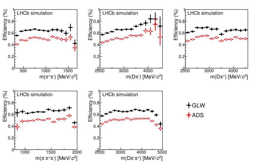
Figure 1: Signal efficiencies for the ${{{B}^{-}}}\rightarrow[{{K}^{-}}{{\pi}^{+}}]_{D}X_{d}^{-}$ decay when applying the GLW and ADS selections. The efficiencies are shown as a function of five different two- and three-body masses.

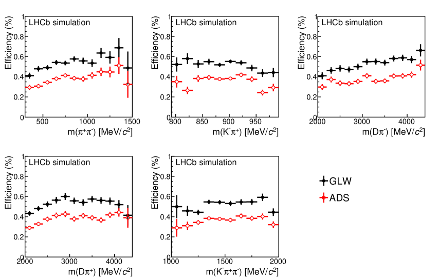
Figure 2: Signal efficiencies for the ${{{B}^{-}}}\rightarrow[{{K}^{-}}{{\pi}^{+}}]_{D}X_{s}^{-}$ decay when applying the GLW and ADS selections. The efficiencies are shown as a function of five different two- and three-body masses.

Figure 3 shows the $X_{d}^{-}$ and $X_{s}^{-}$ invariant mass distributions for ${{{B}^{-}}}\rightarrow[{{K}^{-}}{{\pi}^{+}}]_{D}X_{d}^{-}$ and ${{{B}^{-}}}\rightarrow[{{K}^{-}}{{\pi}^{+}}]_{D}X_{s}^{-}$ signal decays after all selections, except for the $X^{-}$ and ${{K}^{*0}}$ mass requirements. These signal spectra are background subtracted using the sPlot method [44], with the ${{{B}^{-}}}$ candidate invariant mass as the discriminating variable.

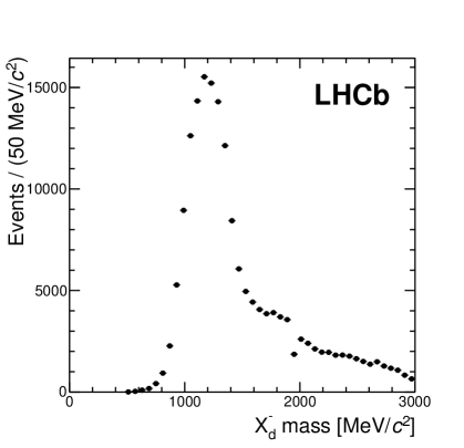
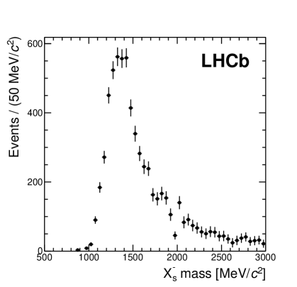
Figure 3: Signal distributions of the (left) $X_{d}^{-}$ invariant mass in ${{{B}^{-}}}\rightarrow DX_{d}^{-}$ decays and (right) $X_{s}^{-}$ invariant mass, in ${{{B}^{-}}}\rightarrow DX_{s}^{-}$ decays, for $D\rightarrow{{K}^{-}}{{\pi}^{+}}$. The distributions are obtained using the sPlot method. In both cases, all selections, except the $M(X^{-})<2$${\mathrm{\,Ge\kern-0.90005ptV\!/}c^{2}}$ and the ${{K}^{*0}}$ mass selection, are applied. The dip at 1.97${\mathrm{\,Ge\kern-0.90005ptV\!/}c^{2}}$ is due to the ${{D}^{+}_{s}}$ meson veto.

The $X_{d}^{-}$ and $X_{s}^{-}$ contributions peak in the region below 2${\mathrm{\,Ge\kern-1.00006ptV\!/}c^{2}}$, consistent with the dominance of resonances such as $a_{1}(1260)^{-}\rightarrow{{\pi}^{-}}{{\pi}^{+}}{{\pi}^{-}}$ to the $X_{d}^{-}$ system, and one or more excited strange resonances contributing to $X_{s}^{-}$. The dip at 1.97${\mathrm{\,Ge\kern-1.00006ptV\!/}c^{2}}$ is due to the ${{D}^{-}_{s}}$ mass veto.

5 Fits to data

The signal yields are determined through a simultaneous unbinned extended maximum likelihood fit to the 16 $B^{\pm}$ candidate invariant mass spectra. These 16 spectra include the four ${{{B}^{-}}}\rightarrow DX_{d}^{-}$ decays, where $D\rightarrow K^{\pm}\pi^{\mp},~{}{{K}^{+}}{{K}^{-}}$ and ${{\pi}^{+}}{{\pi}^{-}}$, the corresponding four charge-conjugate decays, and the set of eight modes where $X_{d}^{-}$ is replaced with $X_{s}^{-}$. The signal and background contributions across these modes are similar, although not identical. Where possible, common signal and background shapes are used; otherwise simulation is used to relate parameters in the lower yield modes to the values obtained from the high yield CF $D\rightarrow K\pi$ modes. Signal and background yields are all independent of one another in the ${{{B}^{+}}}$ and ${{{B}^{-}}}$ mass fits; thus $C\!P$ violation is allowed for all contributions in the mass spectrum. Unless otherwise noted, the shapes discussed below are obtained from simulated decays.

5.1 Signal shapes

The ${{{B}^{-}}}$ mass signal shapes are each parameterized as the sum of a Crystal Ball (CB) shape [45] and a Gaussian ($G$) function,

$${\cal{F}}_{sig}\propto f_{\rm CB}{\rm CB}(m_{B},\sigma_{\rm CB},\alpha_{\rm CB},n)+(1-f_{\rm CB})G(m_{B},\sigma_{g}).$$ (13)

The Gaussian function accounts for the core of the mass distribution, whereas the CB function accounts for the non-Gaussian radiative tail below, and a wider Gaussian resolution component above, the signal peak. A small difference is seen between the shapes for the ${{{B}^{-}}}\rightarrow DX_{d}^{-}$ and ${{{B}^{-}}}\rightarrow DX_{s}^{-}$ decays, and so a different set of signal shape parameters is used to describe each, except for a common value of the fitted ${{{B}^{-}}}$ mass, $m_{B}$. The signal shapes are not very sensitive to the power-law exponent, $n$, which is fixed to 10. The parameters $\alpha_{\rm CB}$, $\sigma_{g}$ and $f_{\rm CB}$ are allowed to vary freely in the fit to the data. From simulation, we find that for all 16 modes, $\sigma_{\rm CB}/\sigma_{g}$ is consistent with 1.90, and this ratio is imposed in the fit. Simulation is also used to relate the mass resolution in the $D\rightarrow{{K}^{+}}{{K}^{-}},~{}{{\pi}^{+}}{{\pi}^{-}}$ modes to that of the $D\rightarrow K\pi$ mode, from which it is found that $\sigma_{g}^{[KK]_{D}X^{-}}=(0.947\pm 0.011)\sigma_{g}^{[K\pi]_{D}X^{-}}$ and $\sigma_{g}^{[\pi\pi]_{D}X^{-}}=(1.043\pm 0.011)\sigma_{g}^{[K\pi]_{D}X^{-}}$. The relations are consistent between the ${{{B}^{-}}}\rightarrow DX_{d}^{-}$ and ${{{B}^{-}}}\rightarrow DX_{s}^{-}$ modes, and are applied as fixed constraints (without uncertainties) in the mass fit.

5.2 Backgrounds and their modeling

The primary sources of background in the mass spectra are partially reconstructed $B\rightarrow D^{(*)}X^{-}$ decays, cross-feed between ${{{B}^{-}}}\rightarrow DX_{d}^{-}$ and ${{{B}^{-}}}\rightarrow DX_{s}^{-}$, and other combinatorial backgrounds. All of the spectra have a contribution from combinatorial background, the shape of which is described by an exponential function. Its slope is taken to be the same for the $C\!P$-conjugate ${{{B}^{-}}}$ and ${{{B}^{+}}}$ decays, but differs among the various $D$ and $X^{-}$ final states.

The main contribution to the partially reconstructed background comes from ${{{B}^{-}}}\rightarrow[{{D}^{0}}{{\pi}^{0}},{{D}^{0}}\gamma]_{{{D}^{*0}}}X^{-}$ or ${{\kern 1.79993pt\overline{\kern-1.79993ptB}{}}{}^{0}}\rightarrow[{{D}^{0}}{{\pi}^{+}}]_{{{D}^{*+}}}X^{-}$ decays, where a pion or photon is not considered when reconstructing the ${{{B}^{-}}}$ candidate. Because the missed pion or photon generally has low momentum, these decays pass the full selection with high efficiency. The shapes of these distributions are modeled using parameterized shapes based on simulated decays. Since the Dalitz structure of these backgrounds is not known, we do not rely entirely on simulation to reproduce the shape of this low-mass component. Instead, the parameters of the shape function that depend on the decay dynamics are allowed to vary freely, and are determined in the fit. The shape parameters for these backgrounds are varied independently for ${{{B}^{-}}}\rightarrow DX_{d}^{-}$ and ${{{B}^{-}}}\rightarrow DX_{s}^{-}$ decays.

Another background contribution which primarily contributes to the ${{{B}^{-}}}\rightarrow DX_{d}^{-}$ ADS suppressed mode is the ${{\kern 1.79993pt\overline{\kern-1.79993ptB}{}}{}^{0}}\rightarrow{{D}^{0}}{{\pi}^{-}}{{\pi}^{+}}{{\pi}^{-}}{{\pi}^{+}}$ decay, where there is no ${{D}^{*+}}$ intermediate state. This decay can contribute to the ADS CF mode if a ${{\pi}^{+}}$ is excluded from the decay, or to the ADS DCS mode if a ${{\pi}^{-}}$ is not considered. The branching fraction for this decay is not known, but the similar CF decay ${{\kern 1.79993pt\overline{\kern-1.79993ptB}{}}{}^{0}}\rightarrow{{D}^{*0}}{{\pi}^{-}}{{\pi}^{+}}{{\pi}^{-}}{{\pi}^{+}}$ is known to have a relatively large branching fraction of $(2.7\pm 0.5)\times 10^{-3}$ [46, 47]. Assuming ${\cal{B}}({{\kern 1.79993pt\overline{\kern-1.79993ptB}{}}{}^{0}}\rightarrow{{D}^{0}}{{\pi}^{-}}{{\pi}^{+}}{{\pi}^{-}}{{\pi}^{+}})\simeq{\cal{B}}({{\kern 1.79993pt\overline{\kern-1.79993ptB}{}}{}^{0}}\rightarrow{{D}^{*0}}{{\pi}^{-}}{{\pi}^{+}}{{\pi}^{-}}{{\pi}^{+}})$, this background contribution is about two orders of magnitude larger than the DCS signal, although it peaks at lower mass than the signal. The selection efficiency and shape of this background are difficult to determine from simulation, since there have not been any studies of this final state to date. Its shape is obtained from simulations that assume a quasi two-body process, ${{\kern 1.79993pt\overline{\kern-1.79993ptB}{}}{}^{0}}\rightarrow{{D}^{0}}R,~{}R\rightarrow{{\pi}^{-}}{{\pi}^{+}}{{\pi}^{-}}{{\pi}^{+}}$, which decays uniformly in the phase space. An ARGUS shape [48] convolved with a Gaussian function provides a good description of this simulated background. Its shape parameters are shared between ${{{B}^{+}}}$ and ${{{B}^{-}}}$ and are allowed to vary freely in the fit, except for the Gaussian width, which is fixed to the expected mass resolution of 15${\mathrm{\,Me\kern-1.00006ptV\!/}c^{2}}$.

The analogous ${{\kern 1.79993pt\overline{\kern-1.79993ptB}{}}{}^{0}}\rightarrow{{D}^{0}}{{K}^{-}}{{\pi}^{+}}{{\pi}^{-}}{{\pi}^{+}}$ decay does not pose the same contamination to the DCS ADS ${{{B}^{+}}}\rightarrow[{{K}^{-}}{{\pi}^{+}}]_{D}X_{s}^{+}$ signal, since a missed ${{\pi}^{-}}$ leads to a ${{{B}^{+}}}\rightarrow{{D}^{0}}{{K}^{-}}{{\pi}^{+}}{{\pi}^{+}}$ candidate, which is not one of the decays of interest. However, in the ${{\kern 1.79993pt\overline{\kern-1.79993ptB}{}}{}^{0}_{s}}\rightarrow[{{K}^{-}}{{\pi}^{+}}]_{D^{0}}{{K}^{+}}{{\pi}^{-}}{{\pi}^{+}}{{\pi}^{-}}$ decay, opposite-sign kaons are natural due to the presence of the $\bar{s}$ quark within the ${{\kern 1.79993pt\overline{\kern-1.79993ptB}{}}{}^{0}_{s}}$ meson. This decay is unobserved, but the similar decay, ${{\kern 1.79993pt\overline{\kern-1.79993ptB}{}}{}^{0}_{s}}\rightarrow{{D}^{0}}{{K}^{+}}{{\pi}^{-}}$, has a relatively large branching fraction of $(1.00\pm 0.15)\times 10^{-3}$ [49]. Based on other $B$-meson decays, one would expect the ${{\kern 1.79993pt\overline{\kern-1.79993ptB}{}}{}^{0}_{s}}\rightarrow{{D}^{0}}{{K}^{+}}{{\pi}^{-}}{{\pi}^{+}}{{\pi}^{-}}$ decay to be at the same level, ${\cal{O}}(10^{-3})$, which is two orders of magnitude larger than the signal. The shape of this background has a similar threshold behavior as for the ${{\kern 1.79993pt\overline{\kern-1.79993ptB}{}}{}^{0}}\rightarrow{{D}^{0}}{{\pi}^{-}}{{\pi}^{+}}{{\pi}^{-}}{{\pi}^{+}}$ decay discussed previously, and therefore its contribution is also modeled from simulated decays using an ARGUS shape convolved with a Gaussian function with freely varying shape parameters.

In the fit, we also model cross-feed between the ${{{B}^{-}}}\rightarrow D^{(*)}X_{d}^{-}$ and ${{{B}^{-}}}\rightarrow DX_{s}^{-}$ decays. The shapes of these cross-feed backgrounds are obtained from simulation. The cross-feed rate is obtained from ${{D}^{*+}}\rightarrow{{D}^{0}}{{\pi}^{+}}$, ${{D}^{0}}\rightarrow{{K}^{-}}{{\pi}^{+}}$ calibration data, reweighted to match the properties of the signal decays. All selection requirements on the ${{{B}^{-}}}\rightarrow DX^{-}$ decays, including $|M({{K}^{-}}{{\pi}^{+}})-M_{{{K}^{*0}}}|<100$${\mathrm{\,Me\kern-1.00006ptV\!/}c^{2}}$ and $M(X^{-})<2$${\mathrm{\,Ge\kern-1.00006ptV\!/}c^{2}}$, are taken into account. In total, we find that 0.66% of ${{{B}^{-}}}\rightarrow DX_{d}^{-}$ are misidentified as ${{{B}^{-}}}\rightarrow DX_{s}^{-}$ for the GLW modes and 0.16% for the ADS modes. The lower value for the ADS modes is due to the tighter PID requirements on the ${{K}^{-}}$ candidate in the $X_{s}^{-}$ system. The cross-feed from ${{{B}^{-}}}\rightarrow DX_{s}^{-}$ into ${{{B}^{-}}}\rightarrow DX_{d}^{-}$ is evaluated in an analogous manner, and is found to be 13.7%. Since the ratio of branching fractions is ${\cal{B}}({{{B}^{-}}}\rightarrow DX_{s}^{-})/{\cal{B}}({{{B}^{-}}}\rightarrow DX_{d}^{-})\simeq 0.09$ [50], the yield of this background is only about 1% of the signal yield.

Other sources of background that contribute to the ${{{B}^{-}}}\rightarrow DX_{s}^{-}$ modes are the ${{{B}^{-}}}\rightarrow{{D}^{0}}[{{K}^{-}}{{K}^{+}}{{\pi}^{-}}]_{{{D}^{-}_{s}}}$ and ${{{B}^{-}}}\rightarrow{{D}^{0}}{{K}^{-}}[{{K}^{+}}{{\pi}^{-}}]_{{{\kern 1.39998pt\overline{\kern-1.39998ptK}{}}{}^{*0}}}$ decays, where the ${{K}^{+}}$ is misidentified as a ${{\pi}^{+}}$ meson. The shapes are similar for these two backgrounds and thus a single shape is used, based on a parameterization of the ${{{B}^{-}}}$ candidate mass distribution in simulated ${{{B}^{-}}}\rightarrow{{D}^{0}}[{{K}^{-}}{{K}^{+}}{{\pi}^{-}}]_{{{D}^{-}_{s}}}$ decays. Taking into account known branching fractions [22], efficiencies from simulation, and ${{K}^{+}}\rightarrow{{\pi}^{+}}$ misidentification rates from ${{D}^{*+}}\rightarrow{{D}^{0}}{{\pi}^{+}}$ calibration data, we expect a contribution of 1.6% of the ${{{B}^{-}}}\rightarrow DX_{s}^{-}$ signal.

5.3 Fit results

The invariant mass spectra for the ${{{B}^{-}}}\rightarrow DX_{s}^{-}$ ADS and GLW signal modes are shown in Figs. 4 and 5, with the corresponding spectra for the ${{{B}^{-}}}\rightarrow DX_{d}^{-}$ normalization modes in Figs. 6 and 7. Results from the fits are superimposed along with the various signal and background components. The fitted yields in the ADS and GLW modes are given in Tables 1 and 2.

Table 1: Fitted yields in the ADS modes with $f=K\pi$, for the signal and corresponding normalization modes.

Decay mode	${{{B}^{-}}}$ yield	${{{B}^{+}}}$ yield
	($N^{f}_{{\rm fit},X_{d}^{-}}$)	($N^{f}_{{\rm fit},X_{d}^{+}}$)
$B^{\pm}\rightarrow DX_{d}^{\pm}$, $D\rightarrow{{K}^{-}}{{\pi}^{+}}$	$36\,956\pm 214$	$37\,843\pm 219$
$B^{\pm}\rightarrow DX_{d}^{\pm}$, $D\rightarrow{{K}^{+}}{{\pi}^{-}}$	$~{}~{}161\pm 20$	$~{}~{}162\pm 20$
	($N^{f}_{{\rm fit},X_{s}^{-}}$)	($N^{f}_{{\rm fit},X_{s}^{+}}$)
$B^{\pm}\rightarrow DX_{s}^{\pm}$, $D\rightarrow{{K}^{-}}{{\pi}^{+}}$	$1234\pm 37$	$1226\pm 37$
$B^{\pm}\rightarrow DX_{s}^{\pm}$, $D\rightarrow{{K}^{+}}{{\pi}^{-}}$	$~{}\,13.0\pm 5.3$	$~{}~{}~{}6.6\pm 4.0$

Table 2: Fitted yields used in the GLW analysis with $f=K^{\pm}\pi^{\pm},~{}{{K}^{+}}{{K}^{-}}$ and ${{\pi}^{+}}{{\pi}^{-}}$, for the signal and corresponding normalization modes.

Decay mode	${{{B}^{-}}}$ yield	${{{B}^{+}}}$ yield
	($N^{f}_{{\rm fit},X_{d}^{-}}$)	($N^{f}_{{\rm fit},X_{d}^{+}}$)
$B^{\pm}\rightarrow DX_{d}^{\pm}$, $D\rightarrow{{K}^{-}}{{\pi}^{+}}$	$45\,213\pm 226$	$46\,488\pm 230$
$B^{\pm}\rightarrow DX_{d}^{\pm}$, $D\rightarrow{{K}^{+}}{{K}^{-}}$	$3899\pm 63$	$4084\pm 65$
$B^{\pm}\rightarrow DX_{d}^{\pm}$, $D\rightarrow{{\pi}^{+}}{{\pi}^{-}}$	$1669\pm 38$	$1739\pm 40$
	($N^{f}_{{\rm fit},X_{s}^{-}}$)	($N^{f}_{{\rm fit},X_{s}^{+}}$)
$B^{\pm}\rightarrow DX_{s}^{\pm}$, $D\rightarrow{{K}^{-}}{{\pi}^{+}}$	$1699\pm 47$	$1744\pm 47$
$B^{\pm}\rightarrow DX_{s}^{\pm}$, $D\rightarrow{{K}^{+}}{{K}^{-}}$	$\,~{}155\pm 14$	$\,~{}171\pm 14$
$B^{\pm}\rightarrow DX_{s}^{\pm}$, $D\rightarrow{{\pi}^{+}}{{\pi}^{-}}$	$\,~{}59\pm 9$	$\,~{}70\pm 9$

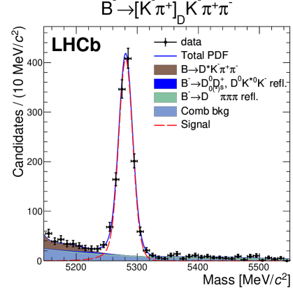
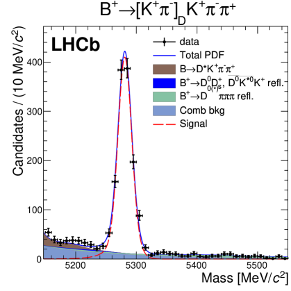
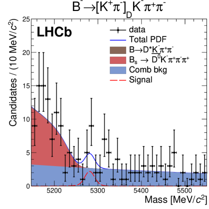
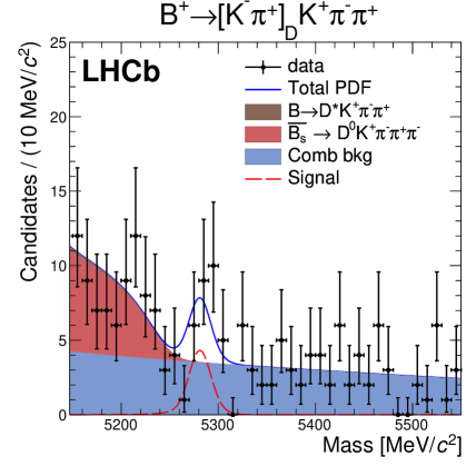
Figure 4: Mass distributions of ${{{B}^{-}}}\rightarrow DX_{s}^{-}$ candidates using the ADS selections, for (top left) ${{{B}^{-}}}\rightarrow[{{K}^{-}}{{\pi}^{+}}]_{D}X_{s}^{-}$, (top right) ${{{B}^{+}}}\rightarrow[{{K}^{+}}{{\pi}^{-}}]_{D}X_{s}^{+}$, (bottom left) ${{{B}^{-}}}\rightarrow[{{K}^{+}}{{\pi}^{-}}]_{D}X_{s}^{-}$, and (bottom right) ${{{B}^{+}}}\rightarrow[{{K}^{-}}{{\pi}^{+}}]_{D}X_{s}^{+}$.

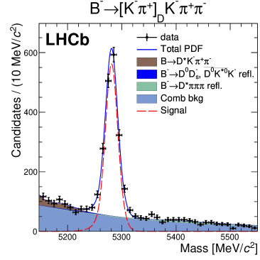
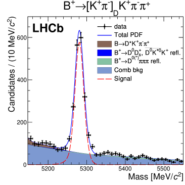
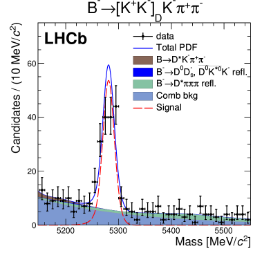
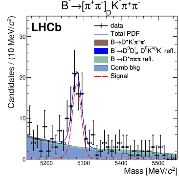
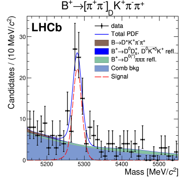
Figure 5: Mass distributions of ${{{B}^{-}}}\rightarrow DX_{s}^{-}$ candidates using the GLW selections, for (top left) ${{{B}^{-}}}\rightarrow[{{K}^{-}}{{\pi}^{+}}]_{D}X_{s}^{-}$, (top right) ${{{B}^{+}}}\rightarrow[{{K}^{+}}{{\pi}^{-}}]_{D}X_{s}^{+}$, (middle left) ${{{B}^{-}}}\rightarrow[{{K}^{+}}{{K}^{-}}]_{D}X_{s}^{-}$, (middle right) ${{{B}^{+}}}\rightarrow[{{K}^{+}}{{K}^{-}}]_{D}X_{s}^{+}$, (bottom left) ${{{B}^{-}}}\rightarrow[{{\pi}^{+}}{{\pi}^{-}}]_{D}X_{s}^{-}$, and (bottom right) ${{{B}^{+}}}\rightarrow[{{\pi}^{+}}{{\pi}^{-}}]_{D}X_{s}^{+}$.

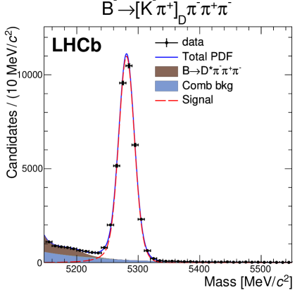
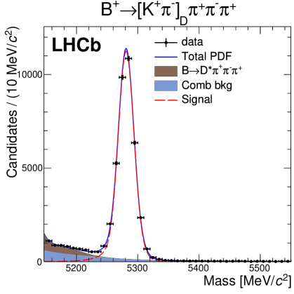
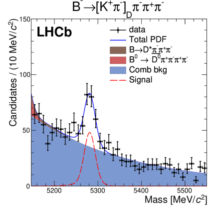
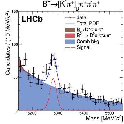
Figure 6: Mass distributions of ${{{B}^{-}}}\rightarrow DX_{d}^{-}$ candidates using the ADS selections, for (top left) ${{{B}^{-}}}\rightarrow[{{K}^{-}}{{\pi}^{+}}]_{D}X_{d}^{-}$, (top right) ${{{B}^{+}}}\rightarrow[{{K}^{+}}{{\pi}^{-}}]_{D}X_{d}^{+}$, (bottom left) ${{{B}^{-}}}\rightarrow[{{K}^{+}}{{\pi}^{-}}]_{D}X_{d}^{-}$, and (bottom right) ${{{B}^{+}}}\rightarrow[{{K}^{-}}{{\pi}^{+}}]_{D}X_{d}^{+}$.

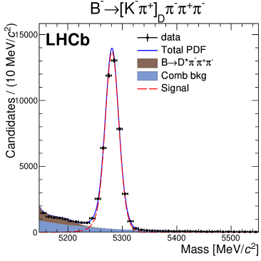
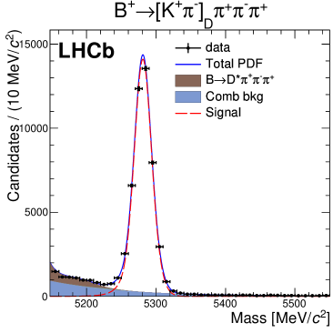
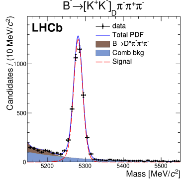
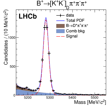
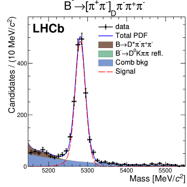
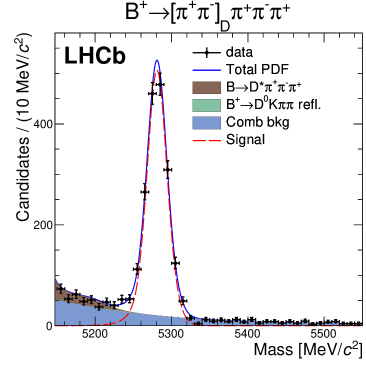
Figure 7: Mass distributions of ${{{B}^{-}}}\rightarrow DX_{d}^{-}$ candidates using the GLW selections, for (top left) ${{{B}^{-}}}\rightarrow[{{K}^{-}}{{\pi}^{+}}]_{D}X_{d}^{-}$, (top right) ${{{B}^{+}}}\rightarrow[{{K}^{+}}{{\pi}^{-}}]_{D}X_{d}^{+}$, (middle left) ${{{B}^{-}}}\rightarrow[{{K}^{+}}{{K}^{-}}]_{D}X_{d}^{-}$, and (middle right) ${{{B}^{+}}}\rightarrow[{{K}^{+}}{{K}^{-}}]_{D}X_{d}^{+}$, (bottom left) ${{{B}^{-}}}\rightarrow[{{\pi}^{+}}{{\pi}^{-}}]_{D}X_{d}^{-}$, and (bottom right) ${{{B}^{+}}}\rightarrow[{{\pi}^{+}}{{\pi}^{-}}]_{D}X_{d}^{+}$

Highly significant signals are seen in all modes, except for the ADS DCS ${{{B}^{-}}}\rightarrow DX_{s}^{-}$ decay. This is the first time these decays have been observed in modes other than the CF ${{D}^{0}}\rightarrow{{K}^{-}}{{\pi}^{+}}$ decay. Figure 8 shows the suppressed ADS mode, $B^{\pm}\rightarrow D[{{K}^{+}}{{\pi}^{-}}]_{D}K^{\pm}\pi^{\mp}\pi^{\pm}$, summed over both $B$-meson charge states. The significance of the peak, which exceeds three standard deviations, is discussed later.

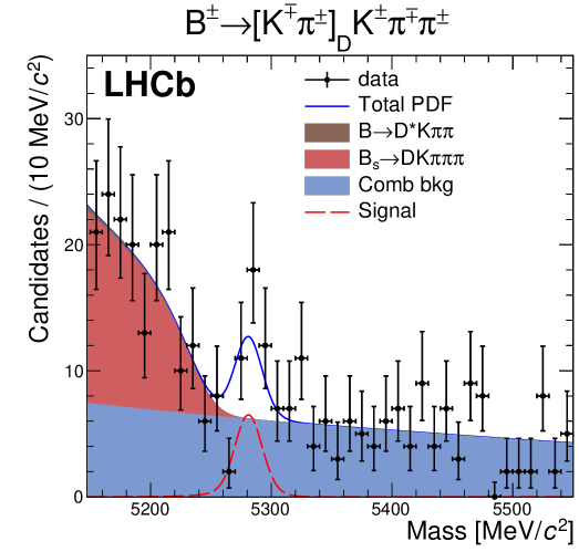
Figure 8: Mass distributions for the suppressed ADS mode, $B^{\pm}\rightarrow[K^{\mp}\pi^{\pm}]_{D}K^{\pm}\pi^{\mp}\pi^{\pm}$ (sum of ${{{B}^{+}}}$ and ${{{B}^{-}}}$).

6 Determination of $C\!P$ observables

The $C\!P$ observables are obtained by expressing the fitted signal yields in terms of corrected yields and the $C\!P$ parameters. For the decay $B^{\pm}\rightarrow f_{D}X_{d}^{\pm}$, where $f_{D}$ is either the ADS CF decay or a $C\!P$ eigenstate, the fitted yields can be written as

$$N^{f}_{{\rm fit},X_{d}^{\pm}}=\frac{1}{2}\Bigg{(}\frac{N_{{\rm corr},X_{d}}^{f}}{1+F^{f}_{\cancel{D},X_{d}}}\Bigg{)}(1\mp{\mathcal{A}}_{{\rm raw},X_{d}}^{f})+C^{f}_{\cancel{c},X_{d}^{\pm}},$$ (14)

where $N_{{\rm corr},X_{d}}^{f}$ is the total corrected yield (sum of ${{{B}^{-}}}$ and ${{{B}^{+}}}$), $F^{f}_{\cancel{D},X_{d}}$ are the estimated fractions of signal events removed by the ${{D}^{0}}$ and $D_{(s)}^{(*)+}$ vetoes, $C^{f}_{\cancel{c},X_{d}^{\pm}}$ are the estimated charmless background yields, and ${\mathcal{A}}_{{\rm raw},X_{d}}^{f}$ is the raw $C\!P$ asymmetry.

The fitted yields in the corresponding $B^{\pm}\rightarrow DX_{s}^{\pm}$ decays are written in terms of the corrected $B^{\pm}\rightarrow DX_{d}^{\pm}$ yields in Eq. 14 and the $C\!P$ observable $R^{f}_{s/d}$ defined in Eqs. 9 and 10, as

$$N^{f}_{{\rm fit},X_{s}^{\pm}}=\frac{1}{2}R^{f}_{s/d}\Bigg{(}\frac{N^{f}_{{\rm corr},X_{d}}}{1+F^{f}_{\cancel{D},X_{s}}}\Bigg{)}(1\mp{\mathcal{A}}_{{\rm raw},X_{s}}^{f})+C^{f}_{\cancel{c},X_{s}^{\pm}},$$ (15)

where the meaning of the symbols parallels those in Eq. 14.

For the ADS suppressed modes, the four DCS yields $N^{K^{\mp}\pi^{\pm}}_{{\rm fit},X^{\pm}}$ are expressed in terms of the corrected CF yields, $N_{{\rm corr},X_{d}}^{K^{\pm}\pi^{\mp}}$, as

$$N^{K^{\mp}\pi^{\pm}}_{{\rm fit},X_{d}^{\pm}}=\left(R^{X_{d}^{\pm}}_{{\rm raw}}\right)\Bigg{(}\frac{N_{{\rm corr},X_{d}}^{K^{\pm}\pi^{\mp}}}{1+F^{K^{\mp}\pi^{\pm}}_{\cancel{D},X_{d}}}\Bigg{)}+C^{K^{\mp}\pi^{\pm}}_{\cancel{c},X_{d}^{\pm}},$$ (16)

$$N^{K^{\mp}\pi^{\pm}}_{{\rm fit},X_{s}^{\pm}}=\left(R^{X_{s}^{\pm}}_{{\rm raw}}\right)\Bigg{(}\frac{N_{{\rm corr},X_{s}}^{K^{\pm}\pi^{\mp}}}{1+F^{K^{\mp}\pi^{\pm}}_{\cancel{D},X_{s}}}\Bigg{)}+C^{K^{\mp}\pi^{\pm}}_{\cancel{c},X_{s}^{\pm}},$$ (17)

where $N_{{\rm corr},X_{s}^{\pm}}^{K^{\pm}\pi^{\mp}}=N_{{\rm corr},X_{s}}^{K^{\pm}\pi^{\mp}}(1\mp{\mathcal{A}}_{{\rm raw},X_{s}}^{K^{\pm}\pi^{\mp}})$ gives the corrected yield for the favored $B^{\pm}\rightarrow[K^{\pm}\pi^{\mp}]_{D}X_{s}^{\pm}$ decays.

The corrections for the ${{D}^{0}}$ and $D_{(s)}^{(*)+}$ vetoes, $F^{f}_{\cancel{D},X_{d,s}}$, are determined by interpolating from the mass regions just above and below the veto region, and lead to corrections that range from 0.6% to 5.8% of the expected yield. Uncertainties on these corrections are considered as sources of systematic uncertainty. Potential contamination from charmless five-body decays is determined by fitting for a $B^{\pm}$ signal component when the $D$ candidates are taken from the ${{D}^{0}}$ mass sideband region, as described previously. The charmless contributions are negligible, and the uncertainties are included in the systematic error. The yields, as determined from the fitted values of the $C\!P$ parameters in Eqs. 14-17, are given in Tables 1 and  2.

The raw observables, ${\mathcal{A}}_{{\rm raw},X}^{f}$ and $R^{X^{\pm}}_{{\rm raw}}$ include small biases due to the production asymmetry of $B^{\pm}$ mesons, ${\cal{A}}_{B^{\pm}}$ (affecting ${\mathcal{A}}_{{\rm raw},X}^{f}$ only), and from the detection asymmetries of kaons and pions, ${\cal{A}}_{K}$ and ${\cal{A}}_{\pi}$. The corrected quantities are then computed according to

$${\mathcal{A}}^{{{K}^{+}}{{K}^{-}}}_{X_{d}} ={\mathcal{A}}^{{{K}^{+}}{{K}^{-}}}_{{\rm raw},X_{d}}-{\cal{A}}_{B^{\pm}}-{\cal{A}}_{\pi},$$ (18)

$${\mathcal{A}}^{{{\pi}^{+}}{{\pi}^{-}}}_{X_{d}} ={\mathcal{A}}^{{{\pi}^{+}}{{\pi}^{-}}}_{{\rm raw},X_{d}}-{\cal{A}}_{B^{\pm}}-{\cal{A}}_{\pi},$$ (19)

$${\mathcal{A}}^{{{K}^{-}}{{\pi}^{+}}}_{X_{d}} ={\mathcal{A}}^{{{K}^{-}}{{\pi}^{+}}}_{{\rm raw},X_{d}}-{\cal{A}}_{B^{\pm}}-{\cal{A}}_{K},$$ (20)

$${\mathcal{A}}^{{{K}^{+}}{{K}^{-}}}_{X_{s}} ={\mathcal{A}}^{{{K}^{+}}{{K}^{-}}}_{{\rm raw},X_{s}}-{\cal{A}}_{B^{\pm}}-{\cal{A}}_{K},$$ (21)

$${\mathcal{A}}^{{{\pi}^{+}}{{\pi}^{-}}}_{X_{s}} ={\mathcal{A}}^{{{\pi}^{+}}{{\pi}^{-}}}_{{\rm raw},X_{s}}-{\cal{A}}_{B^{\pm}}-{\cal{A}}_{K},$$ (22)

$${\mathcal{A}}^{{{K}^{-}}{{\pi}^{+}}}_{X_{s}} ={\mathcal{A}}^{{{K}^{-}}{{\pi}^{+}}}_{{\rm raw},X_{s}}-{\cal{A}}_{B^{\pm}}-2{\cal{A}}_{K}+{\cal{A}}_{\pi},$$ (23)

$$R^{X_{d}^{+}} =R^{X_{d}^{+}}_{{\rm raw}}(1-2{\cal{A}}_{K}+2{\cal{A}}_{\pi}),$$ (24)

$$R^{X_{d}^{-}} =R^{X_{d}^{-}}_{{\rm raw}}(1+2{\cal{A}}_{K}-2{\cal{A}}_{\pi}),$$ (25)

$$R^{X_{s}^{+}} =R^{X_{s}^{+}}_{{\rm raw}}(1-2{\cal{A}}_{K}+2{\cal{A}}_{\pi}),$$ (26)

$$R^{X_{s}^{-}} =R^{X_{s}^{-}}_{{\rm raw}}(1+2{\cal{A}}_{K}-2{\cal{A}}_{\pi}).$$ (27)

The pion detection asymmetry of ${\cal{A}}_{\pi}=0.000\pm 0.003$ is obtained by reweighting the measured $\pi^{\pm}$ detection efficiencies [51] with the expected momentum spectrum for signal pions. The kaon detection efficiency of ${\cal{A}}_{K}=-0.011\pm 0.004$ is obtained by reweighting the measured ${{K}^{-}}\pi$ detection asymmetry [52] using the momentum spectrum of signal kaons, and then subtracting the above pion detection asymmetry. For the production asymmetry, the value ${\cal{A}}_{B^{\pm}}=-0.008\pm 0.007$ is used [53], based on the measured raw asymmetry in $B^{\pm}\rightarrow{{J\mskip-3.0mu/\mskip-2.0mu\psi\mskip 2.0mu}}K^{\pm}$ decays [54] and on simulation.

6.1 Systematic uncertainties

Most potential systematic uncertainties on the observables are expected to cancel in either the asymmetries or ratios that are measured. The systematic uncertainties that do not cancel completely are summarized in Table 3. The PID and trigger asymmetries are evaluated using measured kaon and pion efficiencies from ${{D}^{*+}}\rightarrow{{D}^{0}}{{\pi}^{+}}$ calibration samples in data that are identified using only the kinematics of the decay. The efficiencies for the ${{{B}^{+}}}$ and ${{{B}^{-}}}$ signal decays are then obtained by reweighting the kaon and pion efficiencies using simulated $B^{\pm}\rightarrow DX^{\pm}$ decays to represent the properties of signal data. We find no significant charge asymmetry with respect to the PID requirements, and use ${\cal{A}}_{h}^{\rm PID}=0.000\pm 0.006$, where the uncertainty is dominated by the finite sample sizes of the simulated signal decays in the reweighting. The asymmetry of the hardware trigger is assessed using measured hadron trigger efficiencies in ${{D}^{*+}}\rightarrow{{D}^{0}}{{\pi}^{+}},~{}{{D}^{0}}\rightarrow{{K}^{-}}{{\pi}^{+}}$ decays, reweighted to match the momentum spectrum of tracks from signal decays. Defining the $B^{\pm}$ hadron trigger efficiency as $\epsilon_{B^{\pm}}$, the charge asymmetry of the trigger $(\epsilon_{{{{B}^{-}}}}-\epsilon_{{{{B}^{+}}}})/(\epsilon_{{{{B}^{-}}}}+\epsilon_{{{{B}^{+}}}})$ varies from $0.000\pm 0.003$ for ${{{B}^{-}}}\rightarrow[{{K}^{+}}{{K}^{-}}]_{D}X_{s}^{-}$ to $0.007\pm 0.003$ for ${{{B}^{-}}}\rightarrow[{{K}^{+}}{{\pi}^{+}}]_{D}X_{s}^{-}$. These values are applied as corrections.

Table 3: Systematic uncertainties, in percent, on the fitted parameters.

Source	${\cal{A}}(B^{\pm}\rightarrow DX_{d}^{\pm})$		${\cal{A}}(B^{\pm}\rightarrow DX_{s}^{\pm})$		$R_{{C\!P}+}$		$R_{d}^{\pm}$	$R_{s}^{\pm}$
$D\rightarrow$	$h^{+}h^{-}$	$K\pi$	$h^{+}h^{-}$	$K\pi$	${{K}^{+}}{{K}^{-}}$	${{\pi}^{+}}{{\pi}^{-}}$	$K\pi$	$K\pi$
${\cal{A}}_{B^{\pm}}$	0.7	0.7	0.7	0.7	–	–	–	–
${\cal{A}}_{K}$	–	0.4	0.4	0.8	–	–	0.7	0.7
${\cal{A}}_{\pi}$	0.3	–	–	0.3	–	–	0.6	0.3
Trigger	0.4	0.4	0.4	0.4	1.5	1.5	1.5	1.5
PID	0.6	0.6	0.6	0.6	1.2	1.2	1.2	1.2
Signal model	–	–	–	–	1.1	1.1	–	–
Bkgd. model	–	–	–	–	1.6	1.6	4.0	10.0
Charmless back.	–	–	–	–	1.0	1.0	1.0	1.0
Cross-feed	–	–	–	–	1.0	1.0	1.0	1.0
$D$ vetoes	–	–	–	–	1.0	1.7	1.0	1.0
$R_{{C\!P}+}$ approx.	–	–	–	–	1.0	1.0	–	–
Total	1.0	1.1	1.1	1.3	3.4	3.8	4.9	10.4

On $R_{{C\!P}+}$ and $R^{X^{\pm}}$, we have either a double-ratio or a ratio of final states with identical particles (apart from the charges), and therefore there is a high degree of cancellation of potential systematic uncertainties. We expect that for these ratios, the relative trigger efficiencies would yield a value close to unity. After reweighting the measured trigger efficiencies according to the kinematical properties of signal decays (obtained from simulation), we find that the ratios of trigger efficiencies are within 1.5% of unity, which is assigned as a systematic uncertainty. Using an analogous weighting procedure to the measured PID efficiencies, we find that the relative PID efficiency is equal to unity to within 1.2%, which is assigned as a systematic uncertainty.

We also consider uncertainty from the signal model, the background model, the charmless contamination, the $D$ vetoes, and the detection asymmetries. For the signal model uncertainty, all of the fixed signal shape parameters are varied by one standard deviation, and the resulting changes in the $C\!P$ parameters are added in quadrature to obtain the total signal shape uncertainty (1.1%). For the background-related uncertainties, we consider a polynomial function for the combinatorial background, and vary the fixed background shape parameters of the specific $b$-hadron backgrounds within their uncertainties, and add the deviations from the nominal result in quadrature (1.6%). For the ADS-suppressed modes, larger uncertainties are assigned based on an incomplete understanding of the contributions to the low mass $\bar{B}^{0}_{(s)}\rightarrow{{D}^{0}}X$ background.

The charmless backgrounds are all consistent with zero, and the uncertainty is taken from fits to the $D$ sideband regions (1.0%). Uncertainties due to the cross-feed contributions (such as ${{{B}^{-}}}\rightarrow DX_{d}^{-}$ reconstructed as ${{{B}^{-}}}\rightarrow DX_{s}^{-}$) are assessed using simulated experiments, by simulating the mass distributions with a larger cross-feed and fitting with the nominal value (1.0%). The uncertainties due to vetoing potential contributions from other $D$ mesons are assessed by interpolating the mass spectrum just above and below the veto region into the veto region. The associated uncertainties are all at the 1.0% level, except for the the $B\rightarrow[{{\pi}^{+}}{{\pi}^{-}}]_{D}X_{s}^{-}$ mode, which has an uncertainty of 1.7%.

The uncertainties on the ratios $R_{s/d}^{h^{+}h^{\prime-}}$ and $R^{X_{s,d}^{-}}$ are each summed in quadrature, giving total uncertainties in the range of $(3.4-10.4)\%$, depending on the mode.

7 Results and summary

The resulting values for the $C\!P$ observables are

$$R^{{{K}^{+}}{{K}^{-}}}_{{C\!P}+} =1.043\pm 0.069\pm 0.034,$$

$$R^{{{\pi}^{+}}{{\pi}^{-}}}_{{C\!P}+} =1.035\pm 0.108\pm 0.038,$$

$${\mathcal{A}}^{{{K}^{+}}{{K}^{-}}}_{X_{d}} =-0.019\pm 0.011\pm 0.010,$$

$${\mathcal{A}}^{{{\pi}^{+}}{{\pi}^{-}}}_{X_{d}} =-0.013\pm 0.016\pm 0.010,$$

$${\mathcal{A}}^{{{K}^{-}}{{\pi}^{+}}}_{X_{d}} =-0.002\pm 0.003\pm 0.011,$$

$$R^{X_{d}^{+}} =(43.2\pm 5.3\pm 2.1)\times 10^{-4},$$

$$R^{X_{d}^{-}} =(42.1\pm 5.3\pm 2.1)\times 10^{-4},$$

$${\mathcal{A}}^{{{K}^{+}}{{K}^{-}}}_{X_{s}} =-0.045\pm 0.064\pm 0.011,$$

$${\mathcal{A}}^{{{\pi}^{+}}{{\pi}^{-}}}_{X_{s}} =-0.054\pm 0.101\pm 0.011,$$

$${\mathcal{A}}^{{{K}^{-}}{{\pi}^{+}}}_{X_{s}} =0.013\pm 0.019\pm 0.013,$$

$$R^{X_{s}^{+}} =(107_{-44}^{+60}\pm 11)\times 10^{-4}~{}~{}~{}[~{}<0.018~{}\mbox{\rm at 95\% CL}~{}],$$

$$R^{X_{s}^{-}} =(53_{-42}^{+45}\pm 6)\times 10^{-4}~{}~{}~{}[~{}<0.012~{}\mbox{\rm at 95\% CL}~{}].$$

The values of $R_{{C\!P}+}$ are averaged to obtain

$$R_{{C\!P}+} =1.040\pm 0.064,$$

where the uncertainty includes both statistical and systematic sources, as well as the correlations between the latter.

The significances of the suppressed ADS modes are determined by computing the ratio of log-likelihoods, $\sqrt{2\log({\cal{L}}_{0}/{\cal{L}}_{\rm min})}$, after convolving ${\cal{L}}$ with the systematic uncertainty. From the value of ${\cal{L}}$ at the minimum (${\cal{L}}_{\rm min}$), and the value at $R^{X_{s}^{\pm}}=0$ (${\cal{L}}_{0}$), the significances of the non-zero values for $R^{X_{s}^{-}}$ and $R^{X_{s}^{+}}$ are found to be 2.0$\sigma$ and 3.2$\sigma$, respectively. The overall significance of the observation of the ADS suppressed mode is obtained by adding the log-likelihoods, resulting in a significance of 3.6 standard deviations. This constitutes the first evidence of the ADS suppressed mode in ${{{B}^{-}}}\rightarrow D{{K}^{-}}{{\pi}^{+}}{{\pi}^{-}}$ decays.

For completeness, we also compute the related observables $R_{\rm ADS}$ and ${\mathcal{A}}_{\rm ADS}$, which are commonly used. For the ${{{B}^{-}}}\rightarrow DX_{s}^{-}$ modes, the values are

$$R_{\rm ADS}^{X_{s}} \equiv(R^{X_{s}^{-}}+R^{X_{s}^{+}})/2=(85^{+36}_{-33})\times 10^{-4},$$

$${\mathcal{A}}_{\rm ADS}^{X_{s}} \equiv\frac{R^{X_{s}^{-}}-R^{X_{s}^{+}}}{R^{X_{s}^{-}}+R^{X_{s}^{+}}}=-0.33^{+0.36}_{-0.34}.$$

For the favored modes, the corresponding values are

$$R_{\rm ADS}^{X_{d}} \equiv(R^{X_{s}^{-}}+R^{X_{s}^{+}})/2=(42.7\pm 5.6)\times 10^{-4},$$

$${\mathcal{A}}_{\rm ADS}^{X_{d}} \equiv\frac{R^{X_{s}^{-}}-R^{X_{s}^{+}}}{R^{X_{s}^{-}}+R^{X_{s}^{+}}}=-0.013\pm 0.087.$$

The averages are computed using the asymmetric uncertainty distributions, and include both statistical and systematical sources.

To assess the constraints on $\gamma$ that these observables provide, they have been implemented in the fitter for $\gamma$ described in Ref. [14, *LHCb-CONF-2014-004]. Two fits are performed, one that uses only information from ${{{B}^{-}}}\rightarrow\ DX_{s}^{-}$, and a second that uses the observables from both ${{{B}^{-}}}\rightarrow\ DX_{s}^{-}$ and ${{{B}^{-}}}\rightarrow\ DX_{d}^{-}$ decays. In both fits, the parameters from the $D$-meson system, $r_{D}$, $\delta_{D}^{K\pi}$, $x_{D}$, $y_{D}$, $A^{\rm dir}_{CP}({{K}^{+}}{{K}^{-}})$, and $A^{\rm dir}_{CP}({{\pi}^{+}}{{\pi}^{-}})$, are constrained in an analogous way to what was done for the ${{{B}^{-}}}\rightarrow D{{K}^{-}}$ and ${{{B}^{-}}}\rightarrow D{{\pi}^{-}}$ case [14, *LHCb-CONF-2014-004]. The four parameters $r_{B}$, $\delta_{B}$, $\kappa$ and $\gamma$ are freely varied in each fit. In the combined fit, three additional strong parameters, $r_{B}^{DX_{d}}$, $\delta_{B}^{DX_{d}}$, $\kappa^{DX_{d}}$ are included, which are analogous to those that apply to the ${{{B}^{-}}}\rightarrow\ DX_{s}^{-}$ decay.

The projections of the fit results for $\gamma$, $r_{B}$ and $r_{B}$ versus $\gamma$, are shown in Fig. 9 using the method of Ref. [55] (see also Refs. [14, *LHCb-CONF-2014-004].)

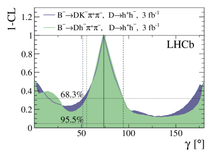
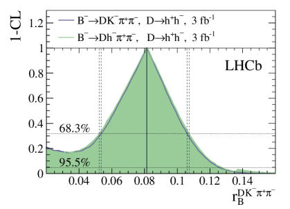
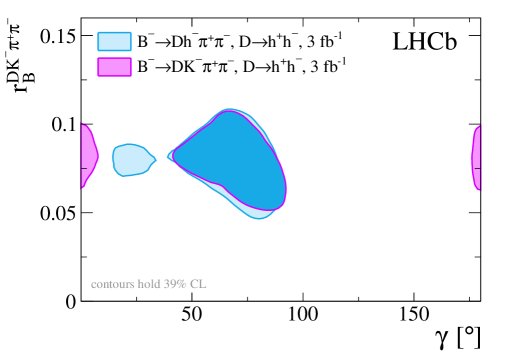
Figure 9: Projections of 1$-$CL versus (left) $\gamma$, (right) $r_{B}^{{{{B}^{-}}}\rightarrow D{{K}^{-}}{{\pi}^{+}}{{\pi}^{-}}}$, and (bottom) $r_{B}^{{{{B}^{-}}}\rightarrow D{{K}^{-}}{{\pi}^{+}}{{\pi}^{-}}}$ versus $\gamma$, using only ${{{B}^{-}}}\rightarrow\ D{{K}^{-}}{{\pi}^{+}}{{\pi}^{-}}$ decays, and the combination of ${{{B}^{-}}}\rightarrow\ D{{K}^{-}}{{\pi}^{+}}{{\pi}^{-}}$ and ${{{B}^{-}}}\rightarrow\ D{{\pi}^{-}}{{\pi}^{+}}{{\pi}^{-}}$ decays. The 68.3% and 95.5% confidence level (CL) limits are indicated for the $\gamma$ and $r_{B}$ projections. The 39% level contours in $r_{B}^{{{{B}^{-}}}\rightarrow D{{K}^{-}}{{\pi}^{+}}{{\pi}^{-}}}$ versus $\gamma$ correspond to the 68.3% level contours in the one-dimensional projections.

The value of $\gamma$ is found to be $(74^{+20}_{-23})^{\rm o}$ for the ${{{B}^{-}}}\rightarrow DX_{s}^{-}$-only fit, and $(74^{+20}_{-19})^{\rm o}$ for the for the combined ${{{B}^{-}}}\rightarrow DX_{s}^{-}$ and ${{{B}^{-}}}\rightarrow DX_{d}^{-}$ fit. The value of $r_{B}$ is nearly identical in the two cases, with corresponding values of $r_{B}=0.081^{+0.025}_{-0.027}$ and $r_{B}=0.081^{+0.026}_{-0.029}$. As expected, most of the sensitivity comes from the ${{{B}^{-}}}\rightarrow DX_{s}^{-}$ decay mode. This value is almost identical to the LHCb combined result of $(73^{+9}_{-10})^{\rm o}$ found in Ref. [14, *LHCb-CONF-2014-004]. The value of $r_{B}$ is similar to the values found in other ${{{B}^{-}}}\rightarrow D{{K}^{-}}$ decays [56, 53, 57, 58, 59], but smaller than the value of $0.240^{+0.055}_{-0.048}$ [60] found in neutral $B$-meson decays. The strong phase $\delta_{B}$, averaged over the phase space, peaks at 172^o for both fits, but at 95% CL all angles are allowed. The constraints on the coherence factor are relatively weak; while the most likely value is close to 1, any value in the interval $[0,1]$ is allowed at one standard deviation.

In summary, a $pp$ collision data sample, corresponding to an integrated luminosity of 3.0 fb^-1, has been used to study the ${{{B}^{-}}}\rightarrow DX_{s}^{-}$ and ${{{B}^{-}}}\rightarrow DX_{d}^{-}$ decay modes, where the $D$ meson decays to either the quasi-flavor-specific $K\pi$ final state or the ${{K}^{+}}{{K}^{-}}$ and ${{\pi}^{+}}{{\pi}^{-}}$ $C\!P$ eigenstates. We observe for the first time highly significant signals in the $C\!P$ modes for both the favored and suppressed ${{{B}^{-}}}$ decays, and we also report the first evidence for the ADS DCS ${{{B}^{-}}}\rightarrow[{{K}^{+}}{{\pi}^{-}}]_{D}{{K}^{-}}{{\pi}^{+}}{{\pi}^{-}}$ decay. We measure the corresponding ADS and GLW observables for the first time in these modes. A fit for $\gamma$ using only these modes is performed, from which we find $\gamma=(74^{+20}_{-23})^{\rm o}$ for the fit with only ${{{B}^{-}}}\rightarrow DX_{s}^{-}$, and $\gamma=(74^{+20}_{-19})^{\rm o}$ for the combined ${{{B}^{-}}}\rightarrow DX_{s}^{-}$ and ${{{B}^{-}}}\rightarrow DX_{d}^{-}$ fit. Values of $\gamma$ below about $25^{\rm o}$ and larger than approximately $165^{\rm o}$ are not excluded by these modes alone, but are excluded when other modes are considered [14, *LHCb-CONF-2014-004]. The precision on $\gamma$ in this analysis is comparable to, or better than, most previous measurements.

LHCb collaboration

R. Aaij³⁸, B. Adeva³⁷, M. Adinolfi⁴⁶, A. Affolder⁵², Z. Ajaltouni⁵, S. Akar⁶, J. Albrecht⁹, F. Alessio³⁸, M. Alexander⁵¹, S. Ali⁴¹, G. Alkhazov³⁰, P. Alvarez Cartelle⁵³, A.A. Alves Jr⁵⁷, S. Amato², S. Amerio²², Y. Amhis⁷, L. An³, L. Anderlini^17,g, J. Anderson⁴⁰, M. Andreotti^16,f, J.E. Andrews⁵⁸, R.B. Appleby⁵⁴, O. Aquines Gutierrez¹⁰, F. Archilli³⁸, P. d’Argent¹¹, A. Artamonov³⁵, M. Artuso⁵⁹, E. Aslanides⁶, G. Auriemma^25,n, M. Baalouch⁵, S. Bachmann¹¹, J.J. Back⁴⁸, A. Badalov³⁶, C. Baesso⁶⁰, W. Baldini^16,38, R.J. Barlow⁵⁴, C. Barschel³⁸, S. Barsuk⁷, W. Barter³⁸, V. Batozskaya²⁸, V. Battista³⁹, A. Bay³⁹, L. Beaucourt⁴, J. Beddow⁵¹, F. Bedeschi²³, I. Bediaga¹, L.J. Bel⁴¹, I. Belyaev³¹, E. Ben-Haim⁸, G. Bencivenni¹⁸, S. Benson³⁸, J. Benton⁴⁶, A. Berezhnoy³², R. Bernet⁴⁰, A. Bertolin²², M.-O. Bettler³⁸, M. van Beuzekom⁴¹, A. Bien¹¹, S. Bifani⁴⁵, T. Bird⁵⁴, A. Birnkraut⁹, A. Bizzeti^17,i, T. Blake⁴⁸, F. Blanc³⁹, J. Blouw¹⁰, S. Blusk⁵⁹, V. Bocci²⁵, A. Bondar³⁴, N. Bondar^30,38, W. Bonivento¹⁵, S. Borghi⁵⁴, M. Borsato⁷, T.J.V. Bowcock⁵², E. Bowen⁴⁰, C. Bozzi¹⁶, S. Braun¹¹, D. Brett⁵⁴, M. Britsch¹⁰, T. Britton⁵⁹, J. Brodzicka⁵⁴, N.H. Brook⁴⁶, A. Bursche⁴⁰, J. Buytaert³⁸, S. Cadeddu¹⁵, R. Calabrese^16,f, M. Calvi^20,k, M. Calvo Gomez^36,p, P. Campana¹⁸, D. Campora Perez³⁸, L. Capriotti⁵⁴, A. Carbone^14,d, G. Carboni^24,l, R. Cardinale^19,j, A. Cardini¹⁵, P. Carniti²⁰, L. Carson⁵⁰, K. Carvalho Akiba^2,38, R. Casanova Mohr³⁶, G. Casse⁵², L. Cassina^20,k, L. Castillo Garcia³⁸, M. Cattaneo³⁸, Ch. Cauet⁹, G. Cavallero¹⁹, R. Cenci^23,t, M. Charles⁸, Ph. Charpentier³⁸, M. Chefdeville⁴, S. Chen⁵⁴, S.-F. Cheung⁵⁵, N. Chiapolini⁴⁰, M. Chrzaszcz⁴⁰, X. Cid Vidal³⁸, G. Ciezarek⁴¹, P.E.L. Clarke⁵⁰, M. Clemencic³⁸, H.V. Cliff⁴⁷, J. Closier³⁸, V. Coco³⁸, J. Cogan⁶, E. Cogneras⁵, V. Cogoni^15,e, L. Cojocariu²⁹, G. Collazuol²², P. Collins³⁸, A. Comerma-Montells¹¹, A. Contu^15,38, A. Cook⁴⁶, M. Coombes⁴⁶, S. Coquereau⁸, G. Corti³⁸, M. Corvo^16,f, B. Couturier³⁸, G.A. Cowan⁵⁰, D.C. Craik⁴⁸, A. Crocombe⁴⁸, M. Cruz Torres⁶⁰, S. Cunliffe⁵³, R. Currie⁵³, C. D’Ambrosio³⁸, J. Dalseno⁴⁶, P.N.Y. David⁴¹, A. Davis⁵⁷, K. De Bruyn⁴¹, S. De Capua⁵⁴, M. De Cian¹¹, J.M. De Miranda¹, L. De Paula², W. De Silva⁵⁷, P. De Simone¹⁸, C.-T. Dean⁵¹, D. Decamp⁴, M. Deckenhoff⁹, L. Del Buono⁸, N. Déléage⁴, D. Derkach⁵⁵, O. Deschamps⁵, F. Dettori³⁸, B. Dey⁴⁰, A. Di Canto³⁸, F. Di Ruscio²⁴, H. Dijkstra³⁸, S. Donleavy⁵², F. Dordei¹¹, M. Dorigo³⁹, A. Dosil Suárez³⁷, D. Dossett⁴⁸, A. Dovbnya⁴³, K. Dreimanis⁵², L. Dufour⁴¹, G. Dujany⁵⁴, F. Dupertuis³⁹, P. Durante³⁸, R. Dzhelyadin³⁵, A. Dziurda²⁶, A. Dzyuba³⁰, S. Easo^49,38, U. Egede⁵³, V. Egorychev³¹, S. Eidelman³⁴, S. Eisenhardt⁵⁰, U. Eitschberger⁹, R. Ekelhof⁹, L. Eklund⁵¹, I. El Rifai⁵, Ch. Elsasser⁴⁰, S. Ely⁵⁹, S. Esen¹¹, H.M. Evans⁴⁷, T. Evans⁵⁵, A. Falabella¹⁴, C. Färber¹¹, C. Farinelli⁴¹, N. Farley⁴⁵, S. Farry⁵², R. Fay⁵², D. Ferguson⁵⁰, V. Fernandez Albor³⁷, F. Ferrari¹⁴, F. Ferreira Rodrigues¹, M. Ferro-Luzzi³⁸, S. Filippov³³, M. Fiore^16,38,f, M. Fiorini^16,f, M. Firlej²⁷, C. Fitzpatrick³⁹, T. Fiutowski²⁷, K. Fohl³⁸, P. Fol⁵³, M. Fontana¹⁰, F. Fontanelli^19,j, R. Forty³⁸, O. Francisco², M. Frank³⁸, C. Frei³⁸, M. Frosini¹⁷, J. Fu²¹, E. Furfaro^24,l, A. Gallas Torreira³⁷, D. Galli^14,d, S. Gallorini^22,38, S. Gambetta⁵⁰, M. Gandelman², P. Gandini⁵⁵, Y. Gao³, J. García Pardiñas³⁷, J. Garofoli⁵⁹, J. Garra Tico⁴⁷, L. Garrido³⁶, D. Gascon³⁶, C. Gaspar³⁸, U. Gastaldi¹⁶, R. Gauld⁵⁵, L. Gavardi⁹, G. Gazzoni⁵, A. Geraci^21,v, D. Gerick¹¹, E. Gersabeck¹¹, M. Gersabeck⁵⁴, T. Gershon⁴⁸, Ph. Ghez⁴, A. Gianelle²², S. Gianì³⁹, V. Gibson⁴⁷, O. G. Girard³⁹, L. Giubega²⁹, V.V. Gligorov³⁸, C. Göbel⁶⁰, D. Golubkov³¹, A. Golutvin^53,31,38, A. Gomes^1,a, C. Gotti^20,k, M. Grabalosa Gándara⁵, R. Graciani Diaz³⁶, L.A. Granado Cardoso³⁸, E. Graugés³⁶, E. Graverini⁴⁰, G. Graziani¹⁷, A. Grecu²⁹, E. Greening⁵⁵, S. Gregson⁴⁷, P. Griffith⁴⁵, L. Grillo¹¹, O. Grünberg⁶³, B. Gui⁵⁹, E. Gushchin³³, Yu. Guz^35,38, T. Gys³⁸, C. Hadjivasiliou⁵⁹, G. Haefeli³⁹, C. Haen³⁸, S.C. Haines⁴⁷, S. Hall⁵³, B. Hamilton⁵⁸, T. Hampson⁴⁶, X. Han¹¹, S. Hansmann-Menzemer¹¹, N. Harnew⁵⁵, S.T. Harnew⁴⁶, J. Harrison⁵⁴, J. He³⁸, T. Head³⁹, V. Heijne⁴¹, K. Hennessy⁵², P. Henrard⁵, L. Henry⁸, J.A. Hernando Morata³⁷, E. van Herwijnen³⁸, M. Heß⁶³, A. Hicheur², D. Hill⁵⁵, M. Hoballah⁵, C. Hombach⁵⁴, W. Hulsbergen⁴¹, T. Humair⁵³, N. Hussain⁵⁵, D. Hutchcroft⁵², D. Hynds⁵¹, M. Idzik²⁷, P. Ilten⁵⁶, R. Jacobsson³⁸, A. Jaeger¹¹, J. Jalocha⁵⁵, E. Jans⁴¹, A. Jawahery⁵⁸, F. Jing³, M. John⁵⁵, D. Johnson³⁸, C.R. Jones⁴⁷, C. Joram³⁸, B. Jost³⁸, N. Jurik⁵⁹, S. Kandybei⁴³, W. Kanso⁶, M. Karacson³⁸, T.M. Karbach^38,†, S. Karodia⁵¹, M. Kelsey⁵⁹, I.R. Kenyon⁴⁵, M. Kenzie³⁸, T. Ketel⁴², B. Khanji^20,38,k, C. Khurewathanakul³⁹, S. Klaver⁵⁴, K. Klimaszewski²⁸, O. Kochebina⁷, M. Kolpin¹¹, I. Komarov³⁹, R.F. Koopman⁴², P. Koppenburg^41,38, M. Korolev³², L. Kravchuk³³, K. Kreplin¹¹, M. Kreps⁴⁸, G. Krocker¹¹, P. Krokovny³⁴, F. Kruse⁹, W. Kucewicz^26,o, M. Kucharczyk²⁶, V. Kudryavtsev³⁴, A. K. Kuonen³⁹, K. Kurek²⁸, T. Kvaratskheliya³¹, V.N. La Thi³⁹, D. Lacarrere³⁸, G. Lafferty⁵⁴, A. Lai¹⁵, D. Lambert⁵⁰, R.W. Lambert⁴², G. Lanfranchi¹⁸, C. Langenbruch⁴⁸, B. Langhans³⁸, T. Latham⁴⁸, C. Lazzeroni⁴⁵, R. Le Gac⁶, J. van Leerdam⁴¹, J.-P. Lees⁴, R. Lefèvre⁵, A. Leflat^32,38, J. Lefrançois⁷, O. Leroy⁶, T. Lesiak²⁶, B. Leverington¹¹, Y. Li⁷, T. Likhomanenko^65,64, M. Liles⁵², R. Lindner³⁸, C. Linn³⁸, F. Lionetto⁴⁰, B. Liu¹⁵, X. Liu³, S. Lohn³⁸, I. Longstaff⁵¹, J.H. Lopes², D. Lucchesi^22,r, M. Lucio Martinez³⁷, H. Luo⁵⁰, A. Lupato²², E. Luppi^16,f, O. Lupton⁵⁵, F. Machefert⁷, F. Maciuc²⁹, O. Maev³⁰, K. Maguire⁵⁴, S. Malde⁵⁵, A. Malinin⁶⁴, G. Manca⁷, G. Mancinelli⁶, P. Manning⁵⁹, A. Mapelli³⁸, J. Maratas⁵, J.F. Marchand⁴, U. Marconi¹⁴, C. Marin Benito³⁶, P. Marino^23,38,t, R. Märki³⁹, J. Marks¹¹, G. Martellotti²⁵, M. Martinelli³⁹, D. Martinez Santos⁴², F. Martinez Vidal⁶⁶, D. Martins Tostes², A. Massafferri¹, R. Matev³⁸, A. Mathad⁴⁸, Z. Mathe³⁸, C. Matteuzzi²⁰, K. Matthieu¹¹, A. Mauri⁴⁰, B. Maurin³⁹, A. Mazurov⁴⁵, M. McCann⁵³, J. McCarthy⁴⁵, A. McNab⁵⁴, R. McNulty¹², B. Meadows⁵⁷, F. Meier⁹, M. Meissner¹¹, M. Merk⁴¹, D.A. Milanes⁶², M.-N. Minard⁴, D.S. Mitzel¹¹, J. Molina Rodriguez⁶⁰, S. Monteil⁵, M. Morandin²², P. Morawski²⁷, A. Mordà⁶, M.J. Morello^23,t, J. Moron²⁷, A.B. Morris⁵⁰, R. Mountain⁵⁹, F. Muheim⁵⁰, J. Müller⁹, K. Müller⁴⁰, V. Müller⁹, M. Mussini¹⁴, B. Muster³⁹, P. Naik⁴⁶, T. Nakada³⁹, R. Nandakumar⁴⁹, I. Nasteva², M. Needham⁵⁰, N. Neri²¹, S. Neubert¹¹, N. Neufeld³⁸, M. Neuner¹¹, A.D. Nguyen³⁹, T.D. Nguyen³⁹, C. Nguyen-Mau^39,q, V. Niess⁵, R. Niet⁹, N. Nikitin³², T. Nikodem¹¹, D. Ninci²³, A. Novoselov³⁵, D.P. O’Hanlon⁴⁸, A. Oblakowska-Mucha²⁷, V. Obraztsov³⁵, S. Ogilvy⁵¹, O. Okhrimenko⁴⁴, R. Oldeman^15,e, C.J.G. Onderwater⁶⁷, B. Osorio Rodrigues¹, J.M. Otalora Goicochea², A. Otto³⁸, P. Owen⁵³, A. Oyanguren⁶⁶, A. Palano^13,c, F. Palombo^21,u, M. Palutan¹⁸, J. Panman³⁸, A. Papanestis⁴⁹, M. Pappagallo⁵¹, L.L. Pappalardo^16,f, C. Parkes⁵⁴, G. Passaleva¹⁷, G.D. Patel⁵², M. Patel⁵³, C. Patrignani^19,j, A. Pearce^54,49, A. Pellegrino⁴¹, G. Penso^25,m, M. Pepe Altarelli³⁸, S. Perazzini^14,d, P. Perret⁵, L. Pescatore⁴⁵, K. Petridis⁴⁶, A. Petrolini^19,j, M. Petruzzo²¹, E. Picatoste Olloqui³⁶, B. Pietrzyk⁴, T. Pilař⁴⁸, D. Pinci²⁵, A. Pistone¹⁹, A. Piucci¹¹, S. Playfer⁵⁰, M. Plo Casasus³⁷, T. Poikela³⁸, F. Polci⁸, A. Poluektov^48,34, I. Polyakov³¹, E. Polycarpo², A. Popov³⁵, D. Popov^10,38, B. Popovici²⁹, C. Potterat², E. Price⁴⁶, J.D. Price⁵², J. Prisciandaro³⁹, A. Pritchard⁵², C. Prouve⁴⁶, V. Pugatch⁴⁴, A. Puig Navarro³⁹, G. Punzi^23,s, W. Qian⁴, R. Quagliani^7,46, B. Rachwal²⁶, J.H. Rademacker⁴⁶, B. Rakotomiaramanana³⁹, M. Rama²³, M.S. Rangel², I. Raniuk⁴³, N. Rauschmayr³⁸, G. Raven⁴², F. Redi⁵³, S. Reichert⁵⁴, M.M. Reid⁴⁸, A.C. dos Reis¹, S. Ricciardi⁴⁹, S. Richards⁴⁶, M. Rihl³⁸, K. Rinnert⁵², V. Rives Molina³⁶, P. Robbe^7,38, A.B. Rodrigues¹, E. Rodrigues⁵⁴, J.A. Rodriguez Lopez⁶², P. Rodriguez Perez⁵⁴, S. Roiser³⁸, V. Romanovsky³⁵, A. Romero Vidal³⁷, M. Rotondo²², J. Rouvinet³⁹, T. Ruf³⁸, H. Ruiz³⁶, P. Ruiz Valls⁶⁶, J.J. Saborido Silva³⁷, N. Sagidova³⁰, P. Sail⁵¹, B. Saitta^15,e, V. Salustino Guimaraes², C. Sanchez Mayordomo⁶⁶, B. Sanmartin Sedes³⁷, R. Santacesaria²⁵, C. Santamarina Rios³⁷, M. Santimaria¹⁸, E. Santovetti^24,l, A. Sarti^18,m, C. Satriano^25,n, A. Satta²⁴, D.M. Saunders⁴⁶, D. Savrina^31,32, M. Schiller³⁸, H. Schindler³⁸, M. Schlupp⁹, M. Schmelling¹⁰, T. Schmelzer⁹, B. Schmidt³⁸, O. Schneider³⁹, A. Schopper³⁸, M. Schubiger³⁹, M.-H. Schune⁷, R. Schwemmer³⁸, B. Sciascia¹⁸, A. Sciubba^25,m, A. Semennikov³¹, I. Sepp⁵³, N. Serra⁴⁰, J. Serrano⁶, L. Sestini²², P. Seyfert¹¹, M. Shapkin³⁵, I. Shapoval^16,43,f, Y. Shcheglov³⁰, T. Shears⁵², L. Shekhtman³⁴, V. Shevchenko⁶⁴, A. Shires⁹, R. Silva Coutinho⁴⁸, G. Simi²², M. Sirendi⁴⁷, N. Skidmore⁴⁶, I. Skillicorn⁵¹, T. Skwarnicki⁵⁹, E. Smith^55,49, E. Smith⁵³, I. T. Smith⁵⁰, J. Smith⁴⁷, M. Smith⁵⁴, H. Snoek⁴¹, M.D. Sokoloff^57,38, F.J.P. Soler⁵¹, F. Soomro³⁹, D. Souza⁴⁶, B. Souza De Paula², B. Spaan⁹, P. Spradlin⁵¹, S. Sridharan³⁸, F. Stagni³⁸, M. Stahl¹¹, S. Stahl³⁸, O. Steinkamp⁴⁰, O. Stenyakin³⁵, F. Sterpka⁵⁹, S. Stevenson⁵⁵, S. Stoica²⁹, S. Stone⁵⁹, B. Storaci⁴⁰, S. Stracka^23,t, M. Straticiuc²⁹, U. Straumann⁴⁰, L. Sun⁵⁷, W. Sutcliffe⁵³, K. Swientek²⁷, S. Swientek⁹, V. Syropoulos⁴², M. Szczekowski²⁸, P. Szczypka^39,38, T. Szumlak²⁷, S. T’Jampens⁴, T. Tekampe⁹, M. Teklishyn⁷, G. Tellarini^16,f, F. Teubert³⁸, C. Thomas⁵⁵, E. Thomas³⁸, J. van Tilburg⁴¹, V. Tisserand⁴, M. Tobin³⁹, J. Todd⁵⁷, S. Tolk⁴², L. Tomassetti^16,f, D. Tonelli³⁸, S. Topp-Joergensen⁵⁵, N. Torr⁵⁵, E. Tournefier⁴, S. Tourneur³⁹, K. Trabelsi³⁹, M.T. Tran³⁹, M. Tresch⁴⁰, A. Trisovic³⁸, A. Tsaregorodtsev⁶, P. Tsopelas⁴¹, N. Tuning^41,38, A. Ukleja²⁸, A. Ustyuzhanin^65,64, U. Uwer¹¹, C. Vacca^15,e, V. Vagnoni¹⁴, G. Valenti¹⁴, A. Vallier⁷, R. Vazquez Gomez¹⁸, P. Vazquez Regueiro³⁷, C. Vázquez Sierra³⁷, S. Vecchi¹⁶, J.J. Velthuis⁴⁶, M. Veltri^17,h, G. Veneziano³⁹, M. Vesterinen¹¹, B. Viaud⁷, D. Vieira², M. Vieites Diaz³⁷, X. Vilasis-Cardona^36,p, A. Vollhardt⁴⁰, D. Volyanskyy¹⁰, D. Voong⁴⁶, A. Vorobyev³⁰, V. Vorobyev³⁴, C. Voß⁶³, J.A. de Vries⁴¹, R. Waldi⁶³, C. Wallace⁴⁸, R. Wallace¹², J. Walsh²³, S. Wandernoth¹¹, J. Wang⁵⁹, D.R. Ward⁴⁷, N.K. Watson⁴⁵, D. Websdale⁵³, A. Weiden⁴⁰, M. Whitehead⁴⁸, D. Wiedner¹¹, G. Wilkinson^55,38, M. Wilkinson⁵⁹, M. Williams³⁸, M.P. Williams⁴⁵, M. Williams⁵⁶, T. Williams⁴⁵, F.F. Wilson⁴⁹, J. Wimberley⁵⁸, J. Wishahi⁹, W. Wislicki²⁸, M. Witek²⁶, G. Wormser⁷, S.A. Wotton⁴⁷, S. Wright⁴⁷, K. Wyllie³⁸, Y. Xie⁶¹, Z. Xu³⁹, Z. Yang³, J. Yu⁶¹, X. Yuan³⁴, O. Yushchenko³⁵, M. Zangoli¹⁴, M. Zavertyaev^10,b, L. Zhang³, Y. Zhang³, A. Zhelezov¹¹, A. Zhokhov³¹, L. Zhong³.

¹Centro Brasileiro de Pesquisas Físicas (CBPF), Rio de Janeiro, Brazil
²Universidade Federal do Rio de Janeiro (UFRJ), Rio de Janeiro, Brazil
³Center for High Energy Physics, Tsinghua University, Beijing, China
⁴LAPP, Université Savoie Mont-Blanc, CNRS/IN2P3, Annecy-Le-Vieux, France
⁵Clermont Université, Université Blaise Pascal, CNRS/IN2P3, LPC, Clermont-Ferrand, France
⁶CPPM, Aix-Marseille Université, CNRS/IN2P3, Marseille, France
⁷LAL, Université Paris-Sud, CNRS/IN2P3, Orsay, France
⁸LPNHE, Université Pierre et Marie Curie, Université Paris Diderot, CNRS/IN2P3, Paris, France
⁹Fakultät Physik, Technische Universität Dortmund, Dortmund, Germany
¹⁰Max-Planck-Institut für Kernphysik (MPIK), Heidelberg, Germany
¹¹Physikalisches Institut, Ruprecht-Karls-Universität Heidelberg, Heidelberg, Germany
¹²School of Physics, University College Dublin, Dublin, Ireland
¹³Sezione INFN di Bari, Bari, Italy
¹⁴Sezione INFN di Bologna, Bologna, Italy
¹⁵Sezione INFN di Cagliari, Cagliari, Italy
¹⁶Sezione INFN di Ferrara, Ferrara, Italy
¹⁷Sezione INFN di Firenze, Firenze, Italy
¹⁸Laboratori Nazionali dell’INFN di Frascati, Frascati, Italy
¹⁹Sezione INFN di Genova, Genova, Italy
²⁰Sezione INFN di Milano Bicocca, Milano, Italy
²¹Sezione INFN di Milano, Milano, Italy
²²Sezione INFN di Padova, Padova, Italy
²³Sezione INFN di Pisa, Pisa, Italy
²⁴Sezione INFN di Roma Tor Vergata, Roma, Italy
²⁵Sezione INFN di Roma La Sapienza, Roma, Italy
²⁶Henryk Niewodniczanski Institute of Nuclear Physics Polish Academy of Sciences, Kraków, Poland
²⁷AGH - University of Science and Technology, Faculty of Physics and Applied Computer Science, Kraków, Poland
²⁸National Center for Nuclear Research (NCBJ), Warsaw, Poland
²⁹Horia Hulubei National Institute of Physics and Nuclear Engineering, Bucharest-Magurele, Romania
³⁰Petersburg Nuclear Physics Institute (PNPI), Gatchina, Russia
³¹Institute of Theoretical and Experimental Physics (ITEP), Moscow, Russia
³²Institute of Nuclear Physics, Moscow State University (SINP MSU), Moscow, Russia
³³Institute for Nuclear Research of the Russian Academy of Sciences (INR RAN), Moscow, Russia
³⁴Budker Institute of Nuclear Physics (SB RAS) and Novosibirsk State University, Novosibirsk, Russia
³⁵Institute for High Energy Physics (IHEP), Protvino, Russia
³⁶Universitat de Barcelona, Barcelona, Spain
³⁷Universidad de Santiago de Compostela, Santiago de Compostela, Spain
³⁸European Organization for Nuclear Research (CERN), Geneva, Switzerland
³⁹Ecole Polytechnique Fédérale de Lausanne (EPFL), Lausanne, Switzerland
⁴⁰Physik-Institut, Universität Zürich, Zürich, Switzerland
⁴¹Nikhef National Institute for Subatomic Physics, Amsterdam, The Netherlands
⁴²Nikhef National Institute for Subatomic Physics and VU University Amsterdam, Amsterdam, The Netherlands
⁴³NSC Kharkiv Institute of Physics and Technology (NSC KIPT), Kharkiv, Ukraine
⁴⁴Institute for Nuclear Research of the National Academy of Sciences (KINR), Kyiv, Ukraine
⁴⁵University of Birmingham, Birmingham, United Kingdom
⁴⁶H.H. Wills Physics Laboratory, University of Bristol, Bristol, United Kingdom
⁴⁷Cavendish Laboratory, University of Cambridge, Cambridge, United Kingdom
⁴⁸Department of Physics, University of Warwick, Coventry, United Kingdom
⁴⁹STFC Rutherford Appleton Laboratory, Didcot, United Kingdom
⁵⁰School of Physics and Astronomy, University of Edinburgh, Edinburgh, United Kingdom
⁵¹School of Physics and Astronomy, University of Glasgow, Glasgow, United Kingdom
⁵²Oliver Lodge Laboratory, University of Liverpool, Liverpool, United Kingdom
⁵³Imperial College London, London, United Kingdom
⁵⁴School of Physics and Astronomy, University of Manchester, Manchester, United Kingdom
⁵⁵Department of Physics, University of Oxford, Oxford, United Kingdom
⁵⁶Massachusetts Institute of Technology, Cambridge, MA, United States
⁵⁷University of Cincinnati, Cincinnati, OH, United States
⁵⁸University of Maryland, College Park, MD, United States
⁵⁹Syracuse University, Syracuse, NY, United States
⁶⁰Pontifícia Universidade Católica do Rio de Janeiro (PUC-Rio), Rio de Janeiro, Brazil, associated to ^2
61Institute of Particle Physics, Central China Normal University, Wuhan, Hubei, China, associated to ^3
62Departamento de Fisica , Universidad Nacional de Colombia, Bogota, Colombia, associated to ^8
63Institut für Physik, Universität Rostock, Rostock, Germany, associated to ^11
64National Research Centre Kurchatov Institute, Moscow, Russia, associated to ^31
65Yandex School of Data Analysis, Moscow, Russia, associated to ^31
66Instituto de Fisica Corpuscular (IFIC), Universitat de Valencia-CSIC, Valencia, Spain, associated to ^36
67Van Swinderen Institute, University of Groningen, Groningen, The Netherlands, associated to <sup>41

a</sup>Universidade Federal do Triângulo Mineiro (UFTM), Uberaba-MG, Brazil
^bP.N. Lebedev Physical Institute, Russian Academy of Science (LPI RAS), Moscow, Russia
^cUniversità di Bari, Bari, Italy
^dUniversità di Bologna, Bologna, Italy
^eUniversità di Cagliari, Cagliari, Italy
^fUniversità di Ferrara, Ferrara, Italy
^gUniversità di Firenze, Firenze, Italy
^hUniversità di Urbino, Urbino, Italy
ⁱUniversità di Modena e Reggio Emilia, Modena, Italy
^jUniversità di Genova, Genova, Italy
^kUniversità di Milano Bicocca, Milano, Italy
^lUniversità di Roma Tor Vergata, Roma, Italy
^mUniversità di Roma La Sapienza, Roma, Italy
ⁿUniversità della Basilicata, Potenza, Italy
^oAGH - University of Science and Technology, Faculty of Computer Science, Electronics and Telecommunications, Kraków, Poland
^pLIFAELS, La Salle, Universitat Ramon Llull, Barcelona, Spain
^qHanoi University of Science, Hanoi, Viet Nam
^rUniversità di Padova, Padova, Italy
^sUniversità di Pisa, Pisa, Italy
^tScuola Normale Superiore, Pisa, Italy
^uUniversità degli Studi di Milano, Milano, Italy
^vPolitecnico di Milano, Milano, Italy
^†Deceased

References

- [1] N. Cabibbo, Unitary symmetry and leptonic decays, Phys. Rev. Lett. 10 (1963) 531
- [2] M. Kobayashi and T. Maskawa, CP violation in the renormalizable theory of weak interaction, Prog. Theor. Phys. 49 (1973) 652
- [3] J. Brod and J. Zupan, The ultimate theoretical error on from decays, JHEP 01 (2014) 051, arXiv:1308.5663
- [4] M. Gronau and D. Wyler, On determining a weak phase from charged B decay asymmetries, Phys. Lett. B265 (1991) 172
- [5] M. Gronau and D. London, How to determine all the angles of the unitarity triangle from and , Phys. Lett. B253 (1991) 483
- [6] D. Atwood, I. Dunietz, and A. Soni, Enhanced CP violation with modes and extraction of the Cabibbo-Kobayashi-Maskawa angle , Phys. Rev. Lett. 78 (1997) 3257, arXiv:hep-ph/9612433
- [7] D. Atwood, I. Dunietz, and A. Soni, Improved methods for observing CP violation in and measuring the CKM phase , Phys. Rev. D63 (2001) 036005, arXiv:hep-ph/0008090
- [8] A. Giri, Y. Grossman, A. Soffer, and J. Zupan, Determining using with multibody decays, Phys. Rev. D68 (2003) 054018, arXiv:hep-ph/0303187
- [9] I. Dunietz, CP violation with self-tagging modes, Phys. Lett. B270 (1991) 75
- [10] I. Dunietz, CP violation with beautiful baryons, Z. Phys. C56 (1992) 129
- [11] Fayyazuddin, decays and violation, Mod. Phys. Lett. A14 (1999) 63, arXiv:hep-ph/9806393
- [12] A. K. Giri, R. Mohanta, and M. P. Khanna, Possibility of extracting the weak phase from decays, Phys. Rev. D65 (2002) 073029, arXiv:hep-ph/0112220
- [13] M. Gronau, Improving bounds on in and , Phys. Lett. B557 (2003) 198, arXiv:hep-ph/0211282
- [14] LHCb collaboration, R. Aaij et al., A measurement of the CKM angle from a combination of analyses, Phys. Lett. B726 (2013) 151, arXiv:1305.2050
- [15] LHCb collaboration, Improved constraints on : CKM2014 update, Sep 2014. LHCb-CONF-2014-004
- [16] BaBar collaboration, J. P. Lees et al., Observation of direct CP violation in the measurement of the Cabibbo-Kobayashi-Maskawa angle with decays, Phys. Rev. D87 (2013) 052015, arXiv:1301.1029
- [17] K. Trabelsi, Study of direct CP in charmed decays and measurements of the CKM angle at Belle, arXiv:1301.2033, presented on behalf of the Belle collaboration at CKM2012, Cincinnati, USA, 28 Sep – 2 Oct 2012
- [18] J. Charles et al., Current status of the Standard Model CKM fit and constraints on new physics, Phys. Rev. D91 (2015) 073007, arXiv:1501.05013
- [19] Heavy Flavor Averaging Group, Y. Amhis et al., Averages of -hadron, -hadron, and -lepton properties as of summer 2014, arXiv:1412.7515, updated results and plots available at http://www.slac.stanford.edu/xorg/hfag/
- [20] BESIII collaboration, M. Ablikim et al., Measurement of the strong phase difference in , Phys. Lett. B734 (2014) 227, arXiv:1404.4691
- [21] M. Rama, Effect of mixing in the extraction of with and decays, Phys. Rev. D89 (2014) 014021, arXiv:1307.4384
- [22] Particle Data Group, K. A. Olive et al., Review of particle physics, Chin. Phys. C38 (2014) 090001
- [23] LHCb collaboration, A. A. Alves Jr. et al., The LHCb detector at the LHC, JINST 3 (2008) S08005
- [24] R. Arink et al., Performance of the LHCb Outer Tracker, JINST 9 (2014) P01002, arXiv:1311.3893
- [25] R. Aaij et al., Performance of the LHCb Vertex Locator, JINST 9 (2014) P09007, arXiv:1405.7808
- [26] M. Adinolfi et al., Performance of the LHCb RICH detector at the LHC, Eur. Phys. J. C73 (2013) 2431, arXiv:1211.6759
- [27] A. A. Alves Jr. et al., Performance of the LHCb muon system, JINST 8 (2013) P02022, arXiv:1211.1346
- [28] LHCb collaboration, R. Aaij et al., LHCb detector performance, Int. J. Mod. Phys. A30 (2015) 1530022, arXiv:1412.6352
- [29] R. Aaij et al., The LHCb trigger and its performance in 2011, JINST 8 (2013) P04022, arXiv:1211.3055
- [30] V. V. Gligorov and M. Williams, Efficient, reliable and fast high-level triggering using a bonsai boosted decision tree, JINST 8 (2013) P02013, arXiv:1210.6861
- [31] T. Sjöstrand, S. Mrenna, and P. Skands, PYTHIA 6.4 physics and manual, JHEP 05 (2006) 026, arXiv:hep-ph/0603175
- [32] T. Sjöstrand, S. Mrenna, and P. Skands, A brief introduction to PYTHIA 8.1, Comput. Phys. Commun. 178 (2008) 852, arXiv:0710.3820
- [33] I. Belyaev et al., Handling of the generation of primary events in Gauss, the LHCb simulation framework, J. Phys. Conf. Ser. 331 (2011) 032047
- [34] D. J. Lange, The EvtGen particle decay simulation package, Nucl. Instrum. Meth. A462 (2001) 152
- [35] P. Golonka and Z. Was, PHOTOS Monte Carlo: A precision tool for QED corrections in and decays, Eur. Phys. J. C45 (2006) 97, arXiv:hep-ph/0506026
- [36] Geant4 collaboration, J. Allison et al., Geant4 developments and applications, IEEE Trans. Nucl. Sci. 53 (2006) 270
- [37] Geant4 collaboration, S. Agostinelli et al., Geant4: A simulation toolkit, Nucl. Instrum. Meth. A506 (2003) 250
- [38] M. Clemencic et al., The LHCb simulation application, Gauss: Design, evolution and experience, J. Phys. Conf. Ser. 331 (2011) 032023
- [39] W. D. Hulsbergen, Decay chain fitting with a Kalman filter, Nucl. Instrum. Meth. A552 (2005) 566, arXiv:physics/0503191
- [40] L. Breiman, J. H. Friedman, R. A. Olshen, and C. J. Stone, Classification and regression trees, Wadsworth international group, Belmont, California, USA, 1984
- [41] R. E. Schapire and Y. Freund, A decision-theoretic generalization of on-line learning and an application to boosting, Jour. Comp. and Syst. Sc. 55 (1997) 119
- [42] LHCb collaboration, R. Aaij et al., Measurement of violation in the three-body phase space of charmless decays, Phys. Rev. D90 112004, arXiv:1408.5373
- [43] LHCb collaboration, R. Aaij et al., Evidence for violation in decays, Phys. Rev. Lett. 113 (2014) 141801, arXiv:1407.5907
- [44] M. Pivk and F. R. Le Diberder, sPlot: A statistical tool to unfold data distributions, Nucl. Instrum. Meth. A555 (2005) 356, arXiv:physics/0402083
- [45] T. Skwarnicki, A study of the radiative cascade transitions between the Upsilon-prime and Upsilon resonances, PhD thesis, Institute of Nuclear Physics, Krakow, 1986, DESY-F31-86-02
- [46] Belle collaboration, G. Majumder et al., Observation of , and , Phys. Rev. D70 (2004) 111103, arXiv:hep-ex/0409008
- [47] CLEO collaboration, K. W. Edwards et al., First observation of decays, Phys. Rev. D65 (2002) 012002, arXiv:hep-ex/0105071
- [48] ARGUS collaboration, H. Albrecht et al., Search for hadronic decays, Phys. Lett. B241 (1990) 278
- [49] LHCb collaboration, R. Aaij et al., Dalitz plot analysis of decays, Phys. Rev. D90 (2014) 072003, arXiv:1407.7712
- [50] LHCb, R. Aaij et al., First observation of the decays and , Phys. Rev. Lett. 108 (2012) 161801, arXiv:1201.4402
- [51] LHCb collaboration, R. Aaij et al., Measurement of the – production asymmetry in 7 TeV collisions, Phys. Lett. B713 (2012) 186, arXiv:1205.0897
- [52] LHCb collaboration, R. Aaij et al., Measurement of asymmetry in and decays, JHEP 07 (2014) 041, arXiv:1405.2797
- [53] LHCb collaboration, R. Aaij et al., Observation of the suppressed ADS modes and , Phys. Lett. B723 (2013) 44, arXiv:1303.4646
- [54] LHCb collaboration, R. Aaij et al., Measurements of the branching fractions and asymmetries of and decays, Phys. Rev. D85 (2012) 091105(R), arXiv:1203.3592
- [55] S. Bodhisattva, M. Walker, and M. Woodroofe, On the unified method with nuisance parameters, Statistica Sinica 19 (2009) 301
- [56] LHCb collaboration, R. Aaij et al., Observation of violation in decays, Phys. Lett. B712 (2012) 203, Erratum ibid. B713 (2012) 351, arXiv:1203.3662
- [57] LHCb collaboration, R. Aaij et al., Measurement of violation and constraints on the CKM angle in with decays, Nucl. Phys. B888 (2014) 169, arXiv:1407.6211
- [58] LHCb collaboration, R. Aaij et al., Measurement of the CKM angle using with , decays, JHEP 10 (2014) 097, arXiv:1408.2748
- [59] LHCb collaboration, R. Aaij et al., A study of violation in with the modes , and , Phys. Rev. D91 (2015) 112014 arXiv:1504.05442
- [60] LHCb collaboration, R. Aaij et al., Measurement of CP violation parameters in decays, Phys. Rev. D90 (2014) 112002, arXiv:1407.8136