The Gaia-ESO Survey: Empirical determination of the precision of stellar radial velocities and projected rotation velocities

Abstract

Context. The Gaia-ESO Survey (GES) is a large public spectroscopic survey at the European Southern Observatory Very Large Telescope.

Aims. A key aim is to provide precise radial velocities ($RV$s) and projected equatorial velocities ($v\sin i$) for representative samples of Galactic stars, that will complement information obtained by the Gaia astrometry satellite.

Methods. We present an analysis to empirically quantify the size and distribution of uncertainties in $RV$ and $v\sin i$ using spectra from repeated exposures of the same stars.

Results. We show that the uncertainties vary as simple scaling functions of signal-to-noise ratio ($S/N$) and $v\sin i$, that the uncertainties become larger with increasing photospheric temperature, but that the dependence on stellar gravity, metallicity and age is weak. The underlying uncertainty distributions have extended tails that are better represented by Student’s t-distributions than by normal distributions.

Conclusions. Parametrised results are provided, that enable estimates of the $RV$ precision for almost all GES measurements, and estimates of the $v\sin i$ precision for stars in young clusters, as a function of $S/N$, $v\sin i$ and stellar temperature. The precision of individual high $S/N$ GES $RV$ measurements is 0.22-0.26 km/s, dependent on instrumental configuration.

1 Introduction

The Gaia-ESO survey (GES) is a large public survey programme carried out at the ESO Very Large Telescope (UT-2 Kueyen) with the FLAMES multi-object instrument (Gilmore et al. 2012; Randich & Gilmore 2013). The survey will obtain high- and intermediate-resolution spectroscopy of $\sim 10^{5}$ stars, the majority obtained at resolving powers of $R\sim 17\,000$ with the GIRAFFE spectrograph (Pasquini et al. 2002). The primary objectives are to cover representative samples of all Galactic stellar populations, including thin and thick disc, bulge, halo, and stars in clusters at a range of ages and Galactocentric radii. The spectra contain both chemical and dynamical information for stars as faint as $V\sim 19$ and, when combined with complementary information from the Gaia satellite, will provide full 3-dimensional velocities and chemistry for a large and representative sample of stars. The GES began on 31 December 2011 and will continue for approximately 5 years. There are periodic internal and external data releases, and at the time of writing, data from the first 18 months of survey operations have been analysed and released to the survey consortium for scientific exploitation – the “second internal data release”, known as iDR2. Part of the same data have also been released to ESO through the second Gaia-ESO phase 3 and will soon be available to the general community.

The GES data products include stellar radial velocities ($RV$) and projected rotation velocities ($v\sin i$). A thorough understanding of the uncertainties in $RV$ and $v\sin i$ is an essential component of many aspects of the GES programme. For instance, the GES data are capable of resolving the kinematics of clusters and star forming regions, but because the $RV$ uncertainties are not negligible compared with the observed kinematic dispersion, an accurate deconvolution to establish intrinsic cluster velocity profiles, mass-dependent kinematic signatures, net rotation etc. relies on a detailed knowledge of the $RV$ uncertainties (e.g. Cottaar, Meyer & Parker 2012; Jeffries et al. 2014; Lardo et al. 2015; Sacco et al. 2015). Searching for binary members of clusters and looking for outliers in $RV$ space also requires an understanding of the uncertainty distribution in order to optimise search criteria and minimise false-positives. Similarly, inverting the projected rotation velocity distribution to a true rotation velocity distribution (e.g. Chandrasekhar & Münch 1950; Dufton et al. 2006) or comparison of the rotation velocity distributions of different samples requires an understanding of how uncertainties in $v\sin i$ broaden the observed distribution and impose a lower limit to the rotation that can be resolved (Frasca et al. 2015).

These examples illustrate that not only does one wish to know the level of uncertainty in $RV$ and $v\sin i$ as a function of stellar spectral type, the spectrum signal-to-noise ratio ($S/N$), the rotation rate and possibly other variables, but it is also important to understand whether the uncertainties are normally distributed or perhaps have extended tails that might be better represented in some other way (e.g. Cottaar et al. 2014). The procedures for reducing and analysing the GES spectra will be fully detailed in forthcoming data release papers, but ultimately the $RV$s and $v\sin i$ are estimated with a detailed chi-squared fitting procedure (Koposov et al. in prep and Sect. 2.3). Fitting uncertainties can of course be computed, but these are often minor contributors to the overall repeatability of the measurements and therefore underestimate the total uncertainty. In this paper we empirically determine the uncertainties and their probability distribution based upon repeated measurements of the same stars in GES. Our analysis is limited to the $>90$ per cent of spectra measured with the GIRAFFE spectrograph and deals only with the precision of the measurements, rather than their absolute accuracy.

In Sect. 2 we describe the GES data and the database of repeat measurements for $RV$ and $v\sin i$ that is available for characterising their uncertainties. In Sect. 3 we show how the differences in $RV$ and $v\sin i$ measured between repeated observations can be used to determine the underlying distribution of measurement uncertainty, represented by simple scaling functions that depend on $S/N$ and $v\sin i$. In Sect. 4 we investigate how these scaling functions alter with stellar properties. Sect. 5 considers how the measurement uncertainties change for different observational configurations within GES. In Sect. 6, we conclude and provide parametric formulae and coefficients that allow an estimation of the $RV$ and $v\sin i$ precision of GES measurements.

2 Repeat measurements of radial velocities and projected rotation velocities

2.1 GES observations

The GES employs the FLAMES fibre-fed, multi-object instrument, feeding both the UVES high-resolution ($R\sim 45\,000$) and GIRAFFE intermediate resolution ($R\sim 17\,000$) spectrographs. More than 90 per cent of the spectra are obtained with GIRAFFE and we deal only with these data here. The Medusa fibre system allows the simultaneous recording of spectra from $\simeq 100$ stars in each pointing. The stars in a single pointing are usually related by scientific interest (a cluster or a bulge field etc.) and cover a limited range of brightness (usually less than a 4 magnitude spread). A further $\simeq 15$ fibres are normally allocated to patches of blank sky.

The GIRAFFE spectrograph permits the recording of a limited spectral range and this is selected through the use of order sorting filters. Eight of these have been used in the GES (HR3, HR5A, HR6, HR10, HR11, HR14A, HR15N, HR21), each of which records a spectrum over a fixed wavelength range, although just three filters (HR10, HR15N, HR21) are used for the large majority of observations:

• Most observations of targets in clusters and star forming regions are made using order sorting filter HR15N. The wavelength range of this filter (6444-6816Å) includes both the H$\alpha$ and lithium lines and can provide useful information on the effective temperature ($T_{\rm eff}$), gravity ($\log g$), age and magnetic activity of the target stars (Lanzafame et al 2015).

• Most targets in the halo, bulge and disc fields are observed using both filters HR10 and HR21. The main goals here are to provide accurate stellar parameters and chemical abundances.

GES fields are usually observed in observation blocks (OBs) comprising two science exposures of equal duration. In addition, for filters HR10 and HR15N a short ”simcal” exposure is interleaved between the science exposures. The “simcal” observation illuminates five dedicated fibres with a Thorium-Argon (ThAr) lamp, providing a means of monitoring the wavelength calibration. In the HR21 observations, this role was fulfilled by emission lines in the sky spectra and no “simcal” exposures were performed.

Table 1: Numbers of short and long term repeat GIRAFFE observations of RV and $v\sin i$ used for open clusters with order sorting filter HR15N.

Name	Age	Ref	Number of repeat observations
	(Myr)		$RV$, $S/N$$>$5		$v\sin i$, $>$5 km s-1
			short	long	short	long
			term	term	term	term
Rho Ophiuchi	1	1	222	33	34	2
Chamaeleon I	2	2	617	81	108	22
Gamma Velorum	6	3	1719	523	382	80
IC4665	30	4	448	25	43	1
NGC2264	3	5	2010	333	717	142
NGC2516	140	6	853	134	266	36
NGC2547	35	7	1045	515	321	164
NGC6633	600	8	1403	243	103	14
Field giants	—		112	9	30	2

2.2 Data reduction

Full details of the GES GIRAFFE data reduction will be given in a forthcoming paper (Lewis et al., in prep.). In brief, the raw data frames are corrected for a bias level using zero exposure bias frames and the resulting images are divided by normalised daytime tungsten lamp exposures to remove pixel-to-pixel sensitivity variations. The multiple spectra in each CCD frame are traced using the tungsten lamp exposures and then extracted using the optimal algorithm described by Horne (1986). Given the readout noise and gain of the CCD, this algorithm also yields an estimated $S/N$ in the extracted spectral pixels, and it is this estimate that is propagated through subsequent analysis steps leading to the final reported $S/N$ of the spectra. Extracted day-time tungsten lamp spectra are used to correct the overall shape of the spectrum and calibrate the individual transmission efficiencies of each fibre. The wavelength calibration proceeded in two stages. Deep exposures of a daytime ThAr lamp are used to define a polynomial relationship between extracted spectral pixel and wavelength. Then, for observations using filters HR10 or HR15N the wavelength calibration is modified by an offset determined from the positions of prominent arc lines in the night-time “simcal” exposures. For observations using filter HR21 the offset applied to the wavelength calibration is determined from the position of prominent emission lines in the sky spectra. Spectra are rebinned into 0.05 Å pixels using this wavelength solution and sky is subtracted using a median of the sky spectra corrected for the differing responses of each fibre.

2.3 Radial velocity and projected rotation velocity estimates

The resulting survey spectra are processed and analysed by working groups organised in a workflow described by Gilmore et al. (2012). The $RV$ and $v\sin i$ estimates used in this report are determined using a pipeline developed by the Cambridge Astronomical Survey Unit (CASU) which follows the general method described by Koposov et al. (2011). Details of the pipeline used to analyse the GES data will be described in a forthcoming paper (Koposov et al. in preparation). A first pass used a standard cross-correlation method with a grid of synthetic template spectra at a range of temperatures, metallicities and gravities (Munari et al. 2005) to give an initial $RV$ estimate. The second pass used a direct modelling approach that fits each spectrum with a low-order polynomial multiplied by a template spectrum, with the $RV$, $v\sin i$, $T_{\rm eff}$, $\log g$, metallicity and polynomial coefficients as free parameters. The best fit parameter set is found by chi-squared minimisation with emission lines excluded from the fitting process. The fitting process is then repeated using a finer grid to determine optimum values of $RV$ and $v\sin i$ with the other parameters held constant at their previously determined values.

The chi-squared minimisation yields an estimate of the uncertainty in the best fit parameters. However, in the case of GES data, this under-estimates the measurement uncertainty, in part due to the analysis step where spectra are re-binned but chiefly due to systematic uncertainties in wavelength calibration (Jeffries et al. 2014). For this reason an empirical determination of the measurement precision is preferred; the measurement uncertainty is estimated by comparing repeated measurements of $RV$ and $v\sin i$ for the same star.

Table 2: Log of VLT/Flames observations used in the analysis of $RV$ and $v\sin i$ measurement precision. The full list is available as Supplementary Material to the on-line version of this paper.

Filter	Date	UT	RA (J2000)	Dec (J2000)	Exposure	Number	Number	Cluster
	observation		field centre	field centre	time (s)	exposures	Targets	code
HR15N	2012-02-15	03:07:58.00	08:10:59.3	-47:37:03.5	600	2	111	gam2vel
HR15N	2012-02-15	03:42:56.00	08:09:20.0	-47:35:46.3	600	2	112	gam2vel
HR15N	2012-02-15	04:18:23.00	08:07:20.6	-47:41:06.0	600	2	81	gam2vel
HR15N	2012-03-15	03:43:29.00	11:21:01.7	-76:23:40.7	600	2	29	Cha-I
HR15N	2012-03-16	01:39:44.00	11:21:01.7	-76:23:40.8	600	2	29	Cha-I

2.4 Selected data

To empirically characterise the $RV$ and $v\sin i$ uncertainties and how they depend on stellar parameters requires a database containing a large number of repeat observations of the same stars and a broad range of stellar types and rotational broadening. For these reasons, and especially to ensure a range of $v\sin i$, we initially focused on GES data for eight open clusters that were observed using the HR15N filter. These clusters have ages in the range 1 to 600 Myr (see Table 1), covering both pre-main sequence and main sequence objects. Only a fraction of the targets in each pointing will be actual cluster members, but we expect that cluster members will dominate any subsample of low-mass stars with high $v\sin i$, since older field stars are not expected to rotate quickly. To provide a sample with older ages and lower gravities, a field consisting mainly of red giants, observed on repeated occasions as part of the GES-CoRoT collaboration, was included.

The data were restricted to observations made with two equal length exposures per OB. Since this is the usual mode of GIRAFFE observations this leads to no significant loss of data. Using this standard arrangement simplifies the analysis and allows two distinct classes of measurement uncertainty to be identified:

• Short-term repeats are where empirical estimates of uncertainties are obtained by comparing $RV$ and $v\sin i$ values for individual targets derived from spectra measured in each of the individual exposures within an OB. The targets are observed using the same Giraffe fibre in the same configuration and are calibrated using the same wavelength solution. In this case the uncertainty is expected to be caused primarily by noise in the target spectra and inherent uncertainties in the reduction and analysis processes. Any drift in wavelength calibration over time, perhaps due to temperature or pressure changes, is expected to be small since the time delay between exposures is always $<$3000 s and normally $<$1500 s; there should also be no movement of the fibres and any effects due to imperfect scrambling in the fibre or changing hour angle (see Sect. 6) should also be small. The assumption is also made that any significant velocity shifts due to binary motion on such short timescales will be rare enough to be neglected.

• Long-term repeats are where uncertainties are estimated by comparing the mean values of $RV$ and $v\sin i$ measured in one OB with those measured for the same target in a second OB, where the fibre allocation and configuration on the plate is changed between OBs. In this case the empirical uncertainties are due to the combined effects of noise in the spectra, the analysis techniques plus any external uncertainties in the wavelength calibration or possibly differences due to the particular fibre used for a target or the hour angle of the observation. Binary motion may also contribute to any observed velocity shifts. A subset of these long-term repeat observations were observations of the same star taken on the same night but in a different fibre configuration. These are invaluable in assessing the relative importance of binaries to the velocity shifts.

  The data used in comparing $RV$ measurements were selected to have $S/N>$5 (for the combined spectra in an OB) and those data used to compare $v\sin i$ have $S/N>$5 and $v\sin i>5$ km s^-1. Table 1 shows the number of short and long term comparisons of $RV$ and $v\sin i$ available for each cluster. Table 2 shows the time, date, field centre co-ordinates, exposure times and numbers of targets for each of the Giraffe OBs used in this paper. Values of $RV$, $v\sin i$, $S/N$ and stellar properties are taken from the iDR2 iteration of analysis of the GES data, first released by the Cambridge Astronomical Unit to the GES working groups in May 2014 and subsequently placed in the GES archive at the Wide Field Astronomy Unit at Edinburgh University.

3 Normalised distributions of measurement uncertainty

Figures 1 and 2 show the general characteristics of the observed RV precision, which is defined by the distribution of $E_{RV}=\Delta RV/\sqrt{2}$, the change in $RV$ between short-term repeat pairs of observations for individual targets divided by $\sqrt{2}$. Figure 1 shows $|E_{RV}|$ for $\sim$8500 short term repeats. There is a strong dependence on $S/N$ and $v\sin i$ such that the measurement precision cannot be represented by a distribution dependent on just one of these parameters. Figure 2 compares the distributions of $E_{RV}$ for short- and long-term repeats. The peak height is reduced and the full width half maximum (FWHM) is increased for long-term repeats. There is thus an apparent increase in measurement uncertainty for targets with high $S/N$ when compared to the precision assessed using short-term repeats of the same stars.

Our general approach is to divide $E_{RV}$ (and the corresponding $E_{v\sin i}$) by some function of the target, signal and spectrograph properties, in order to identify the underlying normalised distributions of measurement precision. If the underlying distributions are Gaussian then these normalising functions, $S_{RV}$ and $S_{v\sin i}$, would correspond to the standard deviations of $E_{RV}$ and $E_{v\sin i}$ as a function of $S/N$, $v\sin i$ and stellar properties. $S_{RV}$ and $S_{v\sin i}$, are used here in a more general sense in order to normalise the $E_{RV}$ and $E_{v\sin i}$ distributions to an as yet unknown underlying distribution which could be non-Gaussian.

Initially, we make the simplifying assumption that the normalising functions depend only on the $S/N$ and $v\sin i$ of the target star and on the spectrum resolution and pixel size, which are set by the GIRAFFE order-sorting filter.

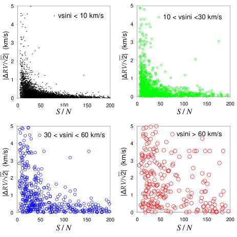
Figure 1: The empirical uncertainty in $RV$ precision ($E_{RV}=\Delta RV/\sqrt{2}$) estimated from the change in $RV$ between short-term repeat observations of cluster targets (see Tables 1 and 2) using order-sorting filter HR15N. The size of the symbol indicates the measured value of $v\sin i$.

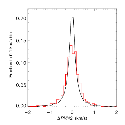
Figure 2: Comparison of the probability density of $E_{RV}$ for short- and long-term repeats (see Tables 1 and 2) using order-sorting filter HR15N. The black line shows results for short-term repeats (i.e. pairs of observations within the same OB). The red histogram shows results for long-term repeats (i.e. spectra of the same targets but taken from different OBs where individual targets are allocated to different fibres).

3.1 Normalising functions

$RV$ and $v\sin i$ are estimated by matching the wavelength offset and line width of a rotationally broadened template spectrum to the measured spectrum. To assess the dependency of uncertainty in $RV$ on $S/N$ and $v\sin i$ it can be shown (see Appendix A) that the distribution of $E_{RV}$ values measured from short term repeats scales approximately according to $W^{3/2}/(S/N)$ where $W$ is the FWHM of individual lines in a template spectrum, rotationally broadened to match the line width of the measured spectrum. In this case (also see Appendix A), the $RV$ precision for short term repeats should scale as

$$S_{RV,0}=B\frac{(1+([v\sin i]/C)^{2})^{3/4}}{S/N}\,,$$ (1)

where $C\approx 0.895c/R_{\lambda}$, $R_{\lambda}$ is the resolving power of the spectrograph, $c$ is the speed of light and $B$ is an empirically determined parameter that will depend on the type of star being observed. This is consistent with the variation of uncertainty in RV with S/N predicted by Butler et al. (1996) for photon limited errors.

In the case of long-term repeats there is an additional contribution to the measurement uncertainty due to variations in wavelength calibration. This is independent of $S/N$ and $v\sin i$ and therefore adds a fixed component $A$ in quadrature to the short term uncertainty such that the distribution of $E_{RV}$ for long-term repeats scales as;

$$S_{RV}=\sqrt{A^{2}+S_{RV,0}^{2}}\,,$$ (2)

where $A$ will be an empirically determined constant and $B$ and $C$ are as defined in Eq. 1.

The relative precision of $v\sin i$ used in this paper is defined as $E_{v\sin i}=\Delta v\sin i/\sqrt{2}\langle v\sin i\rangle$ (i.e. a fractional precision), where $\Delta v\sin i$ is the change between repeat observations and $\langle v\sin i\rangle$ is their mean value. To find the normalising function for the $E_{v\sin i}$ distribution we make the assumption that $W$ increases as a function of $v\sin i$ according to the rotational broadening function given by Gray (1984) and that the uncertainty in $W$ varies as $W^{3/2}/(S/N)$. In this case the uncertainty for short-term repeats (see Appendix A) scales as;

$$S_{v\sin i,0}=\beta\frac{(1+([v\sin i]/C)^{2})^{5/4}}{(S/N)\,([v\sin i]/C)^{2}}\,.$$ (3)

Again, a constant term is added in quadrature to account for additional sources of uncertainty present in the case of long-term repeats, such that the distribution of $E_{v\sin i}$ scales as;

$$S_{v\sin i}=\sqrt{\alpha^{2}+S_{v\sin i,0}^{2}}\,,$$ (4)

where $\alpha$ and $\beta$ will be empirically determined constants and $C$ is the same function of spectral resolution featured in Eq. 1.

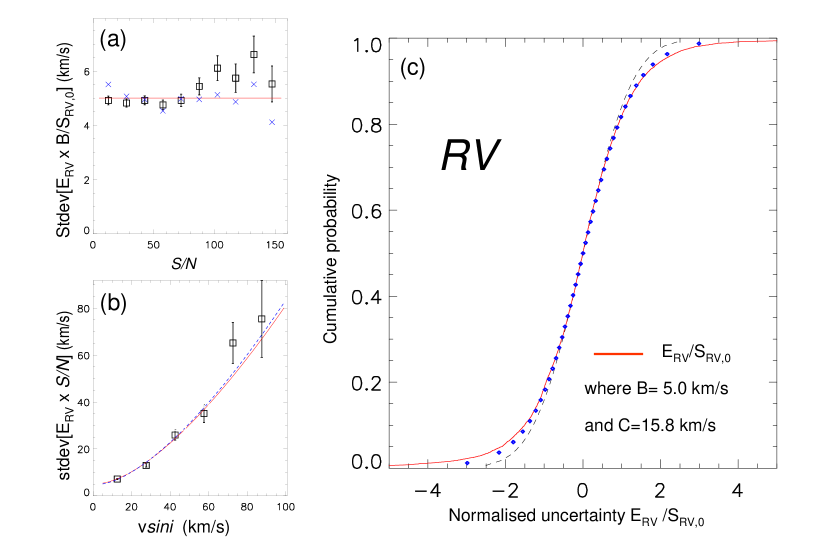
Figure 3: Analysis of the empirical uncertainty for short-term repeat observations of $RV$ using filter HR15N. The solid line in plot (a) shows the variation of $E_{RV}\times(S/N)/(1+([v\sin i]/C)^{2})^{3/4}$ with $S/N$. The horizontal line indicates the value of parameter $B$  in Eq. 1 fitted to the full dataset. Blue crosses show the estimated values $B$ as a function of $S/N$ corrected for the measured variation of $B$ with $T_{\rm eff}$ (see Sect. 4.1 and Table 3). Plot (b) shows the variation of $E_{RV}\times S/N$ with $v\sin i$. The solid line show the relationship predicted using the theoretical value of $C$ and the value of $B$ from plot (a). The dashed line shows a curve of similar functional form using parameters $B$ and $C$ fitted to the binned data. In plots (a) and (b) the y-axis shows an estimate of the standard deviation based on the MAD divided by 0.72 (see Sect. 3.2). Plot (c) shows the cumulative probability distribution (CDF) of the normalised uncertainty in $RV$ for short-term repeats. The red solid line shows results for measured data, the dashed line shows the cumulative distribution of a Gaussian with unit dispersion, and the diamond symbols show the cumulative distribution function for a Student’s t-distribution with $\nu$=6.

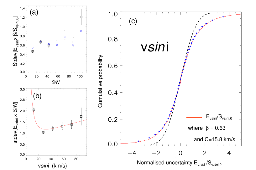
Figure 4: Analysis of the empirical uncertainty for short-term repeat observations of $v\sin i$ using order-sorting filter HR15N. Plot (a) shows the variation of $E_{v\sin i}\times(S/N)([v\sin i]/C)^{2}/(1+([v\sin i]/C)^{2})^{5/4}$ with $S/N$ . The horizontal line indicates the value of parameter $\beta$ in Eq. 3 fitted to the full dataset. Blue crosses show the estimated values $\beta$ as a function of $S/N$ corrected for the measured variation of $\beta$ with $T_{\rm eff}$ (see Sect. 4.4 and Table 3). Plot (b) shows the variation of $E_{v\sin i}\times S/N$ with $v\sin i$. The solid line show the relationship predicted using the theoretical value of $C$ and the value of $\beta$ from plot (a). In plots (a) and (b) the y-axis shows an estimate of the standard deviation based on the MAD divided by 0.82 (for $\nu$=2, see Sect. 3.3). Plot (c) shows the cumulative probability distribution (CDF) of the normalised uncertainty in $v\sin i$ for short-term repeats. The red solid line shows results for measured data, the dashed line shows the cumulative distribution of a Gaussian with unit dispersion, and the diamond symbols show the cumulative distribution function for a Student’s t-distribution with $\nu$=2.

3.2 Parameters for normalising the $RV$ measurement precision

Parameters $A$, $B$ and $C$ defining the normalising function $S_{RV}$ are fitted to match the measured distribution of $E_{RV}$ using a dataset of 8,429 repeat observations, with $S/N>$5, taken using filter HR15N. Since we expect (and it turns out) that the distributions of these quantities are not Gaussians and have significant non-Gaussian tails, we choose to use the median absolute deviation (MAD) to characterise the observed distribution, rather than the square root of the mean variance which could be heavily biased by outliers. An estimate for the standard deviation then follows by noting that the MAD of a Gaussian distribution is 0.674, such that MAD/0.674 gives an estimate of the standard deviation. As we shall see, the distributions more closely follow Student’s t-distributions with $\nu$ degrees of freedom, for which we determine (by Monte Carlo simulation) the corresponding corrections of 0.82 for $\nu=2$, 0.77 for $\nu=3$ and 0.72 for $\nu=6$. Uncertainties in the standard deviations (68 per cent confidence intervals) as a function of sample size are also estimated using the same Monte Carlo simulations.

Defining $A$, $B$ and $C$ is then done in three steps.

1. $B$ is found by finding the MAD of $(E_{RV}\times(S/N)/(1+([v\sin i]/C)^{2})^{3/4}$, using the theoretical value of $C$ determined in Appendix A ($C=15.8$ km s^-1 for filter HR15N, and see step (2) below). Figure 3a shows values of $B$ estimated from data in equal bins of $S/N$. For $S/N<100$ the average values per bin are close to $B=5.0$ km s^-1 for the full data set. There is more scatter for $S/N>100$ but the variation is not excessive considering the larger uncertainties due to the smaller numbers of data per bin. This indicates that the functional form of the normalising function derived in Appendix A is applicable to the GIRAFFE $RV$ data.

2. $C$ is then checked by comparing the curve of $S_{RV,0}\times(S/N)$, calculated using “empirical” values of $B$ and $C$ fitted to the measured values of $E_{RV}\times(S/N)$ as a function of $v\sin i$, with the curve predicted using $B$ and $C$ based on the theoretical value of $C$ determined in Appendix A. Figure 3b shows that these two curves are very similar for the two methods, indicating that the theoretical value of $C$ can be used to predict the scaling of measurement uncertainty in $RV$ with $v\sin i$ . In fact the uncertainty on the fitted slope is largely due to the relatively small proportion of fast rotating stars. For this reason, having confirmed that the data are consistent with the theory in Appendix A, we prefer to use the theoretical value of $C$ rather than an uncertain empirical value. The theoretical value for parameter $C$ is a minimum that assumes any broadening of the spectral lines beyond the spectral resolution is due to rotation. This is reasonable for most types of star in the GES, given the modest resolution of the GIRAFFE spectra, but if $C$ were underestimated then we would over-estimate the increase in measurement uncertainty with $v\sin i$ (see Eq. 1).

   Figure 3c shows the cumulative distribution function (CDF) of $E_{RV}$ for short-term repeats normalised with $S_{RV,0}$, together with the CDF of a unit Gaussian distribution. The distribution of measurement uncertainties follows the Gaussian distribution over the central region ($-1\leq E_{RV}/S_{RV,0}\leq 1$), but larger uncertainties are more frequent than predicted by the Gaussian. The measured distribution of $E_{RV}/S_{RV,0}$ is better represented by a Student’s t-distribution with $\nu=6$ degrees of freedom, $\nu$. This value of $\nu$ represents the integer value that provides the best fit to the normalised uncertainty of short-term repeats at the 5th and 95th percentiles (see Fig. 3). Having determined this, steps (1) and (2) are iterated, dividing the MADs by the appropriate factor of 0.72 (for a Student’s t-distribution with $\nu=6$) to estimate a true standard deviation and produce the final results.

3. The value of $A$ that is added in quadrature to $S_{RV,0}$ is set to $A=0.25\pm 0.02$ km s^-1. This value is chosen so that the normalised CDF of observed $E_{RV}$ found from long-term repeats, $E_{RV}/S_{RV}$, matches the normalised distribution of uncertainty from short-term repeats ($E_{RV}/S_{RV,0}$), but only between the upper and lower quartiles. We choose only to match this range because the tails of the distribution are expected to be different owing to the likely presence of binaries. We show in Sect. 4.3 that this assumption is justified because the distribution of $E_{RV}/S_{RV}$ for those “long-term” repeats where the repeat observations were taken on the same observing night is indistinguishable from that of $E_{RV}/S_{RV,0}$ for short-term repeats both in the core and the tails of the distribution.

   The value of $A$ defines the minimum level of uncertainty that can be achieved for GES spectra with high $S/N$.

Figure 3a shows an increase in the estimated value of $B$ for $S/N>100$. This does not significantly affect the estimate of parameters $A$, $B$ and $C$ described above but does reflect the variation of $B$ with stellar properties. Lower $S/N$ bins contain a mix of stars such that variations of $B$ with stellar properties average out. However the smaller samples in the high $S/N$ bins contain a higher fraction of stars with larger $T_{\rm eff}$ and, as we show in Sect. 4.1, $B$ increases with $T_{\rm eff}$. The blue crosses in Fig. 3a show $T_{\rm eff}$-corrected values $B$ as a function of $S/N$ , using the values discussed in Sect. 4.1 and reported in Table 3. These show a more uniform variation of $B$ with $S/N$.

3.3 Parameters for normalising the $v\sin i$ precision

Constants $\alpha$, $\beta$ and $C$ that define the normalising function $S_{v\sin i}$ are fitted to match the measured distribution of $E_{v\sin i}$ for a subset of the data comprising 2004 observations with $v\sin i>5$ km s^-1. Again, parameters are evaluated in three steps with the MAD being used to estimate the true standard deviations and the analysis being iterated once the true distribution of $E_{v\sin i}/S_{v\sin i}$ is known.

1. First $\beta$ is found by determining the MAD of $E_{v\sin i}(S/N)([v\sin i]/C)^{2}/(1+([v\sin i]/C)^{2})^{5/4}$, using the theoretical value of $C$ determined in Appendix A. The variation of the uncertainty with $S/N$ shows some scatter (see Fig.4a) and consequently there is an $\pm$8 per cent uncertainty in the estimated value of $\beta$.

2. $C$ is then checked by comparing the measured values of $E_{v\sin i}\times(S/N)$  as a function of $v\sin i$ with the curve predicted using $\beta$ and $C$ based on the theoretical value of $C$ determined in Appendix A. Figure 4b shows reasonable agreement between the semi-empirical curve and the measured data indicating that a scaling function of the form $S_{v\sin i}$ using the theoretical value of $C$ can be used to predict the variation of measurement uncertainty with $S/N$ and $v\sin i$.

   Figure 4c shows the CDF of $E_{v\sin i}/S_{v\sin i,0}$ for short-term repeats. This shows a more pronounced tail than the normalised distribution of $E_{RV}$ precision (Fig. 3c) such that a broader Student’s t-distribution with $\nu$=2 is a better fit to the CDF between the 5th and 95th percentiles.

3. Finally, the value of $\alpha$ that represents the effect of wavelength uncertainty for long term repeats is found by matching the normalised $E_{v\sin i}/S_{v\sin i}$ distribution from 463 long-term repeats with the equivalent distribution for the short-term repeats between the upper and lower quartiles, giving $\alpha=0.047\pm 0.003$. This corresponds to the minimum fractional uncertainty in $v\sin i$ that can be obtained from GES spectra with high $S/N$ and large $v\sin i$. This optimum result is most readily achieved in spectra with $v\sin i=2C$ (i.e. 31 km s^-1). Figure 4b shows that, for a given (S/N), fractional uncertainties rise at both higher and lower values of $v\sin i$, and rise drastically for $v\sin i<10$ km s^-1 due to the limited spectral resolution.

Figure 4a shows an increase in the estimated value of $\beta$ for $S/N>100$ due to the higher proportion of hotter stars in this bin. This variation is reduced when the estimated value of $\beta$ is corrected for the measured variation of $\beta$ with $T_{\rm eff}$ discussed in Sect. 4.4 and reported in Table 3.

4 The Effect of Stellar Properties

In Sect. 3 the constants defining the normalising functions $S_{RV}$ and $S_{v\sin i}$ were estimated by fitting data from an inhomogeneous set of stars. The values obtained represent average values. In this section we determine how these “constants” vary with stellar properties, in particular $T_{\rm eff}$, gravity, metallicity, and age. We make the simplifying assumption that uncertainties in $RV$ and $v\sin i$ scale with $S/N$ and $v\sin i$ as described in the last section and that only the parameters $B$ in Eq. 1 and $\beta$ in Eq. 3 depend on stellar properties. This follows because parameters $A$ and $\alpha$ represent uncertainties due to changes in wavelength calibration with time and fibre configuration, and parameter $C$ should depend only on the spectral resolution (Eq. A4).

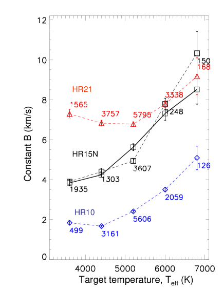
Figure 5: Variation of parameter $B$ of the scaling function for uncertainty in $RV$ ($S_{RV}$) with effective temperature. The solid line shows results for filter HR15N as a function of $T_{\rm eff}$ (see section 4.1). Dashed lines show results for filters HR10, HR15N and HR21 as a function of the temperature of the template spectrum fitted in the CASU pipeline (see Sect. 2.3). Numbers equal the sample size per bin.

4.1 Variation of $S_{RV}$ with effective temperature

Values of $T_{\rm eff}$ determined from an analysis of the iDR2 spectra are available in the GES archive for 75 per cent of HR15N targets considered in this paper. It is labelled Teff in the archive. The $E_{RV}$ values are divided between 5 evenly spaced bins of temperature between 3000 K and 7000 K and analysed as described in section 3.2. The results in Fig. 5 show a slow increase of $B$ with temperature for $T_{\rm eff}<5200$ K such that $B$ is within $\pm$10 per cent of the mean value in Fig. 3b. However, above 5200 K, $B$ increases rapidly with temperature to twice its mean value at $T_{\rm eff}\sim 7000$ K.

The dashed lines in Fig. 5 also show results plotted as a function of the ”template” temperature (known in the GES archive as logTeff). This is the logarithm of the temperature of the best-fit synthetic spectrum that was used to determine $RV$ and $v\sin i$ in the pipeline. This is likely to be less accurate than the $T_{\rm eff}$ derived from a full spectral analysis, but a key advantage is that it is available for all iDR2 targets with a $RV$ and $v\sin i$. In fact, the $B$ values estimated using the ”template” temperature have a very similar trend with $T_{\rm eff}$ and so may be used directly to estimate temperature-dependent values of $B$ and $S_{RV}$ where these are required.

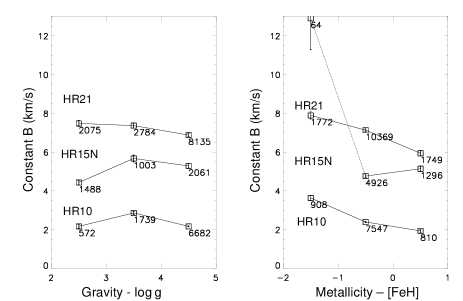
Figure 6: Variation of parameter $B$ of the scaling function for uncertainty in $RV$ ($S_{RV}$) with $\log g$ and metallicity for order sorting filters, HR10, HR15N and HR21. (a) shows the value of $B$ determined for data in three equal bins of $\log g$. Numbers indicate the sample size. (b) shows the value of $B$ determined for data in three equal bins of [Fe/H]. For filter HR15N only the values shown in the upper two bins are reliable due to the low number of targets with [Fe/H]$<$-1.

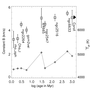
Figure 7: Variation of parameter $B$ of the scaling function for uncertainty in $RV$ ($S_{RV}$) with target age for observations with order sorting filter HR15N. Square symbols show the value of $B$ for targets identified as possible cluster members from their $RV$ versus the nominal age of the cluster (see Table 1). No selection by $RV$ is made for NGC6633 or COROT and we assume the stars have mean ages $>1$ Gyr. The dotted line indicates the median value of $T_{\rm eff}$ (right hand axis values) for members identified in each cluster.

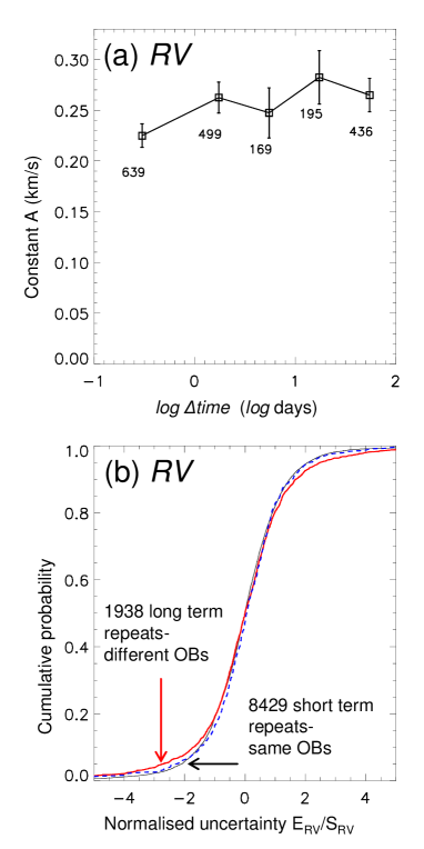
Figure 8: The dependence of the scaling function for uncertainty in $RV$ ($S_{RV}$) as a function of time between observations. Plot (a) shows how scaling parameter $A$ varies with time between repeat observations. Numbers indicate size of the sample used to determine A. Plot (b) shows the CDFs of the normalised distribution of $RV$ precision for short-term repeats (black line), long-term repeats (red line) and long term repeats where the observations were taken on the same observing night (blue dashed line). The CDFs for the short-term repeats and the long-term repeats within a night are indistinguishable using a two-tailed Kolmogorov-Smirnov test.

4.2 Variation of $S_{RV}$ with gravity, metallicity and age

Values of $\log g$ and [Fe/H] (labelled as logg and FeH in the GES archive) obtained from a detailed spectral analysis by the GES working groups are presently available for about 75 percent of the targets observed with order sorting filter HR15N. Analysing these data in bins of $\log g$ (see Fig. 6a) shows only a $\sim$25 percent change in the estimated value of parameter $B$ over a 2 dex range in $\log g$. Analysis in bins of [Fe/H] (see Fig. 6b) shows a similarly small change in $B$ with metallicity over the range of metallicities -1$<$[Fe/H]$<$1. Below this, the estimated value of parameter $B$ appears to increase sharply with decreasing [Fe/H] but in truth there are too few data points for filter HR15N with [Fe/H]$<$-1 to estimate parameter $B$ with any degree of accuracy. We confirmed that any variation seen in Fig. 6 is not due to differences in temperature – the median values of logTeff are very similar in all binned subsamples.

Although the fundamental cause of any variation of $RV$ precision with age would likely be due to the evolution of $\log g$ in pre-main sequence stars, it is nevertheless important to confirm that the prescription for calculating $RV$ precision is valid at all ages, since studying the dynamics of young clusters is a key GES objective. Figure 7 shows the variation of $B$ with stellar age. The adopted ages for cluster stars are those given in Table 1. For this plot, we attempted to separate genuine cluster members from field objects by selecting according to $RV$. For most cluster datasets there was a clear $RV$ peak corresponding to the cluster, so cluster members were selected from a range $\pm$5 km s^-1 either side of this peak with little contamination. However, no selection by $RV$ was made for the COROT sample or for the cluster NGC6633, since neither showed a clear peak in their $RV$ distributions. We assume these datasets contain mostly older ($>1$ Gyr) field stars. Figure 7 shows in any case that there is a weak dependence of $B$ on age. However, it can be seen that this small variation is directly linked to the decreasing median temperatures of the cluster samples at younger ages.

4.3 Variation of $S_{RV}$ with time between observations

In our model of $RV$ uncertainty we assume that $A$ represents some additional uncertainty arising from random changes in wavelength calibration with time and the effects of changes in fibre allocation. We fitted $A$, using the interquartile range of the uncertainty distribution in long-term repeats, in an effort to avoid modelling tails that might be due to binary motion. This simplifying assumption can be tested by plotting values of $A$ determined for samples with increasing time differences between observations. Figure 8a shows that the value of $A$ depends only weakly on the time between observations, increasing from $0.23\pm 0.02$ km s^-1 for measurements made in different configurations on the same night to $0.26\pm 0.02$ km s^-1 for intervals of up to 100 days between observations. This confirms that the $A$ value is not unduly influenced by any binaries in the sample.

The effect of binaries is far more apparent in the tails of the distributions. Figure 8b compares CDFs of the normalised distribution of measurement uncertainty derived from the change in $RV$ between short-term repeats, normalised with $S_{RV,0}$ (Eq. 1), with (i) all the long-term repeats, with uncertainties normalised to $S_{RV}$ (Eq. 2); (ii) a separate distribution of $E_{RV}/S_{RV}$ for just those long-term repeats where the repeat observations were on the same night (nullifying the effects of all but the rarest, short-period binaries). By design, the three CDFs are very close in the interquartile range; but while the CDF for long-term repeats has a more pronounced tail, better described by a Student’s t-distribution with $\nu$=3, the long-term repeats within a night are indistinguishable (with a Kolmogorov-Smirnov test) from the short-term repeats, following a Student’s t-distribution with $\nu=6$. This is consistent with a fraction of the sample being binary stars that show genuine $RV$ changes between observations on timescales longer than a day. It also justifies an assumption that the true uncertainties in a single RV measurent are best represented by the $\nu=6$ Student’s t-distribution multiplied by $S_{RV}$ as given by Eq. 2.

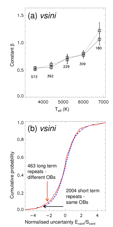
Figure 9: Variation of the scaling function for $v\sin i$ with temperature and time between observations. Plot (a) shows how the $\beta$ parameter in Eq. 3 varies with $T_{\rm eff}$. The solid line shows results using $T_{\rm eff}$ from a detailed spectral analysis; the dashed line shows the results using the ”template” temperature (see Sect. 4.4). Labels indicate the sample size per bin. Plot (b) shows the CDF of the normalised distributions of $v\sin i$ uncertainty for short and long term repeats. Also shown (as small diamonds) is a Student’s t-distribution with $\nu$=2.

4.4 Variation of $S_{v\sin i}$ with temperature and time between observations

In Fig. 9a we show how $\beta$, the parameter in the scaling function governing $v\sin i$ precision (see Eq.3), depends on stellar temperature and the time between observations . The data were divided into 5 equal bins of temperature. Results are shown using the temperature derived from detailed spectral analysis (Teff) and the best-fitting ”template” temperature (logTeff). There appears to be little variation with $T_{\rm eff}$ below 6000 K using either temperature estimate, but like the parameter $B$ governing $RV$ precision, there is a rapid growth in $\beta$ for hotter stars – by about a factor of 2 at $T_{\rm eff}\simeq 7000$ K.

Figure 9b compares the CDF of the normalised measurement precision in $v\sin i$ for short- and long-term repeats. There is much less difference between these CDFs than that found between the short- and long-term repeat estimates of $RV$ precision. This is not unexpected since measurements of $v\sin i$ should be much less effected by binarity. A Student’s t-distribution with $\nu=2$ fits either the short- or long-term repeat CDFs equally well.

There are too few stars in our sample with $v\sin i>5$ km s^-1 for a detailed investigation of how $\beta$ might vary with age, $\log g$ or metallicity subsets.

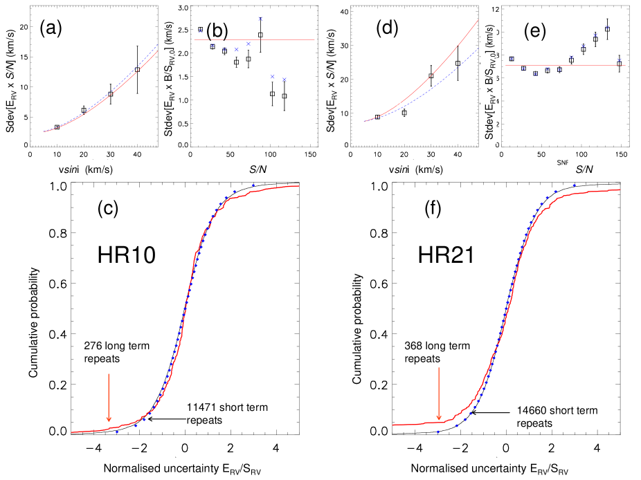
Figure 10: Analysis of the empirical uncertainty for short term repeat observations of $RV$ using filter HR10 and HR21. Plots a and d show the variation of $E_{RV}$ with $v\sin i$. Red lines show the curves predicted using the model value of $C$ (see Eq. A4). The dashed lines shows the curves predicted using values of $B$ and $C$ fitted to the binned data. Plots b and e show the variation in the estimated value of parameter $B$ in Eq. 1 with $S/N$. Red lines show values of $B$ fitted to the full data set for each filter. Blue crosses show the estimated values $B$ as a function of $S/N$ corrected for the measured variation of $B$ with $T_{\rm eff}$ (see Table 3). Plots c and f shows the normalised uncertainty for short term repeats and long term repeats. The black curve shows the CDF for short-term repeats. The red line shows the CDF for long-term repeats. Blue diamonds show a Student’s t-distribution with $\nu=6$, which matches the distribution for short-term repeats well.

Table 3: Constants describing the scaling function of measurement precision in $RV$ and $v\sin i$ as a function of $S/N$ and $v\sin i$ (see Eqns. 2 and 4).

Characteristics of order sorting filter
Filter	HR10	HR15N	HR21
Mean $\lambda$ (Å)	5470	6630	8728
Resolution	19800	17000	16200
Range $\lambda$ (Å)	270	370	504
Parameters defining the scaling function $S_{RV}$ (Eq. 3)
A (km s-1)	0.22$\pm$0.02	0.25$\pm$0.02	0.26$\pm$0.02
C (km s-1)	13.6	15.8	16.6
Average value of $B$ for the mix of stars analysed in this paper
B (km s-1)	2.3	5.0	7.1
Variation of $B$ with template temperature (section 4.1)
B (3200-4000 K)	1.8$\pm$0.2	3.9$\pm$0.1	7.3$\pm$0.2
B (4000-4800 K)	1.7$\pm$0.1	4.4$\pm$0.2	6.8$\pm$0.2
B (4800-5600 K)	2.4$\pm$0.1	4.9$\pm$0.1	6.8$\pm$0.1
B (5600-6400 K)	3.5$\pm$0.2	7.8$\pm$0.3	7.8$\pm$0.2
B (6400-7200 K)	5.1$\pm$0.6	10.3$\pm$1.1	9.2$\pm$1.0
Parameters defining the scaling function $S_{v\sin i}$ (Eq. 4)
$\alpha$	—-	0.047$\pm$0.005	—-
C (km s-1)	—-	15.8	—-
Average value of $\beta$ for the mix of stars analysed in this paper
$\beta$		0.63
Variation of $\beta$ with template temperature (section 4.4)
$\beta$ (3200-4000 K)	—-	0.51$\pm$0.02	—-
$\beta$ (4000-4800 K)	—-	0.60$\pm$0.04	—-
$\beta$ (4800-5600 K)	—-	0.69$\pm$0.08	—-
$\beta$ (5600-6400 K)	—-	0.80$\pm$0.06	—-
$\beta$ (6400-7200 K)	—-	1.22$\pm$0.15	—-
* Where C is calculated from Eq. 4 assuming a limb darkening
coefficient $u=0.6$  (Claret Diaz-Cordoves & Gimenez 1995).

5 Measurement uncertainties using different instrumental configurations

So far the analyses have been restricted to observations with the HR15N order-sorting filter. In this section we consider how these results can be extended to the other GES observational setups. We used all of the “GES_MW” (GES Milky Way Programme) fields, consisting of more than 20,000 $RV$ measurements from individual spectra taken with the HR10 and HR21 filters. Unfortunately there are too few measurements through these filters with $v\sin i>5$ km s^-1 to constrain the $v\sin i$ precision in the same way that was done for HR15n observations.

These precision of the HR10 and HR21 $RV$ measurements were compared with those predicted using the simple model described in Appendix A. For this comparison it is assumed that:

• The uncertainty in $RV$ precision scales as $S_{RV}$ (See Sect. 3.1)

• Parameter $C$ characterising the dependence of $RV$ uncertainty on $v\sin i$ depends on the spectral resolution as $0.895c/R_{\lambda}$ (see Eq. A4).

• Parameter $A$ that determines the difference in $RV$ precision for short- and long-term repeats corresponds to a displacement of the spectrum on the detector in the dispersion direction, measured in pixels, rather than a fixed velocity difference. The number of physical CCD pixels contributing each spectrum along the dispersion direction is 4096, so $\delta_{pix}=4096\overline{\lambda}A/c\Delta\lambda$ where $\Delta\lambda$ is the wavelength range of the filter (see Table 3). In the case of filter HR15, $A=0.25$ km s^-1 corresponds to $\delta_{pix}=0.061$ pixels, which we will assume is the same for the other filters.

Only constant $B$ has to be found, and this can be done using the distribution of $E_{RV}$ found from short-term repeats. This allows the measurement precision of $RV$ for a given filter to be estimated even when there are no long-term repeat measurements to make an independent empirical analysis. In the case of filters HR10 and HR21 it turns out that there are enough long-term repeat measurements, albeit over a restricted range of $v\sin i$ values, to test this hypothesis.

Figure 10 shows an analysis for all field stars that were observed in the GES_MW fields. Figures 10a and d show the variation of the standard deviation of $E_{RV}\times S/N$ with $v\sin i$. Data with large $v\sin i$ values are few; therefore the error bars become large with increasing $v\sin i$. Even so, the curve corresponding to the value of $B$ evaluated for the full data set using the value of $C$ predicted from Eq. A4 is consistent with the empirically measured uncertainties.

Figures 10b and e show how the standard deviation of $(E_{RV})(S/N)/(1+([v\sin i]/C)^{2})^{3/4}$ (estimated using the MAD) varies with $S/N$. For $S/N<100$ both plots show reasonable agreement (within 10 percent) between the measured data and the line showing a single value of $B$ evaluated for the full data set using theroretical $C$. Agreement is less good for data with $S/N>100$. However, any inaccuracy here will have little effect on the estimated uncertainty in $RV$ for the majority of stars which are slow rotators since, at high values of $S/N$, the uncertainty of these stars is dominated by the constant term, $A$ in the expresssion for $S_{RV}$ (see eqns. 1 and 2).

The mean values of $B$ are 2.3 km s^-1 for filter HR10 and 7.1 km s^-1 for filter HR21, compared with 5.0 km s^-1 for HR15N i.e for spectra with similar $v\sin i$ and $S/N$ $RV$s estimated from spectra taken with HR10 are more precise. The temperature dependence, illustrated in Fig. 5, is also different in detail. Figures 6a and b show the variation of $B$ with $\log g$ and [Fe/H]. The trends are similar to the variation found for order sorting filter HR15N i.e $B$ is almost independent of gravity and changes only slowly with metallicity.

Parameter $A$ was determined in two ways. First, it was determined using the measured data for the relatively small sample of long-term repeats as described in Sect. 3.1. This gave values of $A=0.18\pm 0.02$ km s^-1 for filter HR10 and $0.28\pm 0.02$ km s^-1 for filter HR21. These compare with the predicted values of 0.22 km s^-1 and 0.26 km s^-1 inferred by scaling the $\delta_{pix}$ value determined for filter HR15N by the ratio of their pixel sizes in km s^-1.

Figures 10c and 10f shows the CDFs of the normalised uncertainty for short- and long-term repeats using filters HR10 and HR21 respectively. In each case $S_{RV}$ is evaluated using the appropriate theoretical values of $A$ and $C$ and the mean empirical value of $B$ determined for each filter, and these are inserted into Eqns. 1 (for short-term repeats) or 2 (for long-term repeats). Also shown is the CDF of a Student’s t-distribution with $\nu=6$ which, as for the HR15N data, appears to be an excellent representation of the distribution due to short-term repeats. The data are sparse for long-term repeats, but the distributions appear to have more extended tails, consistent with the idea that they contain RV shifts due to binary systems. We do not have sufficient data to test whether the uncertainty CDFs for long-term repeats within a night are similar to those for short-term repeats, but we assume that, like the HR15N data, this will the case for data taken with HR10 and HR21.

6 Discussion and Summary

We have shown that the normalisation functions given in Eqs. (1) –(4) are reasonable descriptions of how uncertainties in $RV$ and $v\sin i$ scale with $S/N$ and $v\sin i$. The recommended average parameters of $A$, $B$, $C$ defining the scaling function for $RV$ are given in Table 3 for observations performed with the three main instrumental configurations used for GIRAFFE observations in the GES. Average values of $\alpha$, $\beta$, and $C$ that define the scaling function for $v\sin i$ are also given for filter HR15N. The uncertainties given by Eqns. 2 and 4 are not normally distributed; they have more extended tails. The uncertainty distribution for a given observation of $RV$ is better represented by the value of Eq. 2 multiplied by a normalised Student’s t-distribution with $\nu=6$, whilst for $v\sin i$ the uncertainty distribution can be approximated by Eq. 4 multiplied by a normalised Student’s t-distribution with $\nu=2$.

Equations 2 and 4 decouple the influences of spectral type and the spectrograph; $A$, $C$ and $\alpha$ are properties of the instrumental setup, whilst $B$ and $\beta$ depend on the type of star observed. The dependence on gravity, age and metallicity, over the range $-1<$[Fe/H]$<1$, is weak; but the temperature dependence becomes strong for $T_{\rm eff}>5200$ K, such that $B$ and $\beta$ increase with $T_{\rm eff}$ and the precision worsens. This is presumably the result of a decreasing number of strong, narrow lines in the spectra of hotter stars. The temperature dependent $B$ and $\beta$ values are listed in Table 3 and should be used in conjunction with the mean values of $A$, $C$ and $\alpha$. There are insufficient observations of stars with $v\sin i>5$ km s^-1 using order-sorting filters HR10 and HR21, so we cannot estimate $\beta$ for such observations. It should also be noted that for reasons of sample size, the calibration of $B$ and $\beta$ is limited to $3200\leq T_{\rm eff}\leq 7200$ K.

Parameter $A$ is between 0.22 and 0.26 km s^-1, dependent on instrumental setup, and represents the best precision with which $RV$ can be obtained from an individual GES spectrum with low rotational broadening and large $S/N$. The origin of this term is unclear; it partly arises from uncertainties in the wavelength calibration and the application of calibration offsets from the “simcal” fibres or sky emission lines. However, various tests have shown these cannot be entirely responsible and we suspect there are additional contributions that may be associated with movement of the fibres at the spectrograph slit assembly or target mis-centering in the fibres combined with imperfect signal scrambling.

The analyses we present were derived from results in the iDR2 GES data release and the coefficients in Table 3 are applicable to those data and also to the more recent iDR3 update that used the same pipeline analysis. The exact use of these results depends on the purpose of any particular investigation. To estimate what approximates to a particular confidence interval on a $RV$ ($v\sin i$) value, the following procedure is recommended:

1. Use the instrumental setup and an estimated stellar temperature (preferably from the GES analysis) to choose the appropriate values of $B$ ($\beta$) and $C$ from Table 3; calculate $S_{RV,0}$ ($S_{v\sin i,0}$) from Eq. 1 (Eq. 3) using the measured $v\sin i$ and $S/N$.

2. Choose the $A$ ($\alpha$) value appropriate for the instrumental setup from Table 3 and calculate $S_{RV}$ ($S_{v\sin i}$) from Eq. 2 (Eq. 4).

3. If combining results from repeated observations, these should be weighted using $S_{RV,0}^{-2}$ ($S_{v\sin i,0}^{-2})$ for short-term repeats (i.e. without the inclusion of the $A$ ($\alpha$) term), or $S_{RV}^{-2}$ ($S_{v\sin i}^{-2}$) for long-term repeats.

4. For accurate modelling of $RV$ data one should use $S_{RV}$ ($S_{v\sin i}$) multiplied by a Student’s t-distribution with $\nu=6$ ($\nu=2$) as a probability distribution for the uncertainty. More crudely, a confidence interval can be estimated by multiplying $S_{RV}$ ($S_{v\sin i}$) by the appropriate percentile point of a Student’s t-distribution with $\nu=6$ ($\nu=2$). For example, to estimate a 68.3 per cent error bar, multiply by 1.09 (1.32), or for a 95.4 per cent error bar multiply by 2.51 (4.50).

Note that whilst the 68.3 per cent confidence intervals are quite close to the value expected for a normal distribution with a standard deviation of $S_{RV}$ ($S_{V\sin i}$), the 95.4 per cent confidence intervals are significantly larger due to the broader tails of the Student’s t-distributions. We do not recommend extrapolating these estimates to even larger confidence intervals since we have few data with which to reliably constrain the distribution at these values. It seems likely that at the conclusion of GES there will be sufficient data (roughly 5 times as much) to significantly improve this situation. A larger dataset will also allow us to study how $v\sin i$ precision varies with $T_{\rm eff}$ and $\log g$ and between differing observational setups.

Appendix A Variation of measurement precision with radial and projected rotation velocities

We consider below how the measurement precision of $RV$ and $v\sin i$ scale with $S/N$ and $v\sin i$ for short-term repeats where there are no changes in setup or wavelength calibration between observations. We make the simplifying assumption that the precision in $RV$ scales as $E_{RV}\propto W^{3/2}/(S/N)$ where $W$, is the FWHM of a Gaussian profile representing the characteristic absorption line profile of the measured spectrum. This approximate relation can be deduced from the results of Landman, Roussel-Dupre and Tanigawa (1982). These authors showed that, for the ideal case of a Gaussian line profile of amplitude $a$, mean value $m$, and standard deviation $s$, sampled using binned data with a uniform Gaussian noise of rms amplitude $\epsilon$ per bin, the statistical uncertainties in the estimated values of $m$ and $s$ are given by;

$$\sigma_{m}=s\left(\frac{4}{\pi}\right)^{1/4}\left(\frac{\Delta x}{s}\right)^{1/2}\left(\frac{\epsilon}{a}\right)\,\,{\rm and}\,\,\sigma_{s}=\sigma_{m}$$ (5)

where $\Delta_{x}$ is the uniform bin width and $\Delta_{x}<<s$.

In the present case $a$ varies with equivalent width, $(EW)$, of the characteristic absorption line as $a=(EW)h/\sqrt{2\pi}\,s$, where $h$ is the amplitude of the contiuum. If the depth of the absortion line, $a$, is small compared to the continuum, $h$ then measurement uncertainty is $\epsilon\approx h/(S/N)$. Substituting these values in equation A1 using the relation $W=\sqrt{8\ln 2}\,s$ gives;

$$\sigma_{m}\propto\left(\frac{\Delta x^{1/2}}{EW}\right)\frac{W^{3/2}}{S/N}\,{\rm and}\,\sigma_{W}\propto\left(\frac{\Delta x^{1/2}}{EW}\right)\frac{W^{3/2}}{S/N}$$ (6)

A.1 Effect of $v\sin i$ on FWHM of the absorption line

For a slowly rotating star, assuming that any sources of broadening other than rotation are much smaller than the intrinsic spectrograph resolution, the FWHM of an individual absorption line is $W_{0}=\overline{\lambda}/R_{\lambda}$, where $\overline{\lambda}$ is the mean wavelength and $R_{\lambda}$ the resolving power of the spectrograph. For fast rotating stars the width of the spectral lines is increased by rotational broadening. Gray (1984) gives the rotational broadening kernel as

$$K(\lambda)=\frac{1}{\Lambda}\left(\frac{2(1-u)/\pi}{(1-u/3)}\sqrt{1-\left(\frac{\lambda}{\Lambda}\right)^{2}}+\frac{u/2}{(1-u/3)}\left(1-\left(\frac{\lambda}{\Lambda}\right)^{2}\right)\right),$$ (7)

where $\Lambda=\overline{\lambda}[v\sin i]/c$, $\lambda$ is wavelength (over the range $-\Lambda<\lambda<\Lambda$) and $u$ is the limb darkening coefficient.

Convolving a spectrum with this kernel increases the FWHM of individual lines approximately as $W\simeq\sqrt{W_{0}^{2}+(8\ln 2)\lambda_{rms}^{2}}$ where $\lambda_{rms}$ is the rms of the broadening kernel ($\lambda_{rms}^{2}=\int\lambda^{2}Kd\lambda$). Evaluating $\gamma_{rms}$ from Eq. A3 gives;

$$W=W_{0}\left(1+\left(\frac{v\sin i}{C}\right)^{2}\right)^{1/2}$$ (8)

where $C=\left(\frac{1-u/3}{1-7u/15}\right)^{1/2}\frac{c}{R_{\lambda}\sqrt{2\ln 2}}$

A.2 Scaling of uncertainty in $RV$ and $v\sin i$

To determine how the uncertainty in radial velocity, $E_{RV}$ scales with $S/N$ and $v\sin i$ we assume $E_{RV}\propto\sigma_{m}$. For a given spectra $\Delta x$ and $EW$ are independent of $W$ and $S/N$ so that (from eqns. A2 and A4) $E_{RV}$ scales with $v\sin i$ and $S/N$ as ,

$$S_{RV,0}=B\frac{\left(1+([v\sin i]/C)^{2}\right)^{3/4}}{S/N}$$ (9)

where $B$ is an empirically determined constant and $C$ depends on $R_{\lambda}$ and $u$. A value of $u=0.6$ is used in this paper (Claret Diaz-Cordoves & Gimenez 1995) giving $C=0.895c/R_{\lambda}$.

The uncertainty in the estimated value of $v\sin i$ is determined from the uncertainty in the estimated absorption line width, $\sigma_{W}$ (eqns. A2 and A4) as;

$$\sigma_{v\sin i}=\frac{C\,W\,\sigma_{W}}{W^{2}_{0}\sqrt{W^{2}/W^{2}_{0}-1}}$$ (10)

Using this expession the uncertainty in the normalised value of $v\sin i$, ( $\propto\sigma_{v\sin i}/[v\sin i]$) scales with $v\sin i$ and $S/N$ as;

$$S_{v\sin i,0}=\beta\frac{\left(1+([v\sin i]/C)^{2}\right)^{5/4}}{(S/N)([v\sin i]/C)^{2}}\,,$$ (11)

where $\beta$ is an empirically determined constant.