Constraining the Braking Indices of Magnetars

Abstract

Due to the lack of long term pulsed emission in quiescence and the strong timing noise, it is impossible to directly measure the braking index $n$ of a magnetar. Based on the estimated ages of their potentially associated supernova remnants (SNRs), we estimate the values of the mean braking indices of eight magnetars with SNRs, and find that they cluster in a range of $1\sim$42. Five magnetars have smaller mean braking indices of $1<n<3$, and we interpret them within a combination of magneto-dipole radiation and wind aided braking, while the larger mean braking indices of $n>3$ for other three magnetars are attributed to the decay of external braking torque, which might be caused by magnetic field decay. We estimate the possible wind luminosities for the magnetars with $1<n<3$, and the dipolar magnetic field decay rates for the magnetars with $n>3$ within the updated magneto-thermal evolution models. Although the constrained range of the magnetars’ braking indices is tentative, due to the uncertainties in the SNR ages, which come from distance uncertainties and the unknown conditions of the expanding shells, our method provides an effective way to constrain the magnetars’ braking indices if the measurements of the SNRs’ ages are reliable, which can be improved by future observations.

1 Introduction

Pulsars are commonly recognized as magnetized neutron stars (NSs), sometimes have been argued to be quark stars (Zheng et al., 2006; Xu, 2007; Lai et al., 2013). A pulsar’s secular spin-down is mainly caused by its rotational energy losses due to electromagnetic radiation, particle winds, star-disk interaction, intense neutrino emission or gravitational radiation (e.g., Peng et al. 1982; Harding et al. 1999; Alpar & Baykal 2006; Chen & Li 2006). An important and measurable quantity closely related to a pulsar’s rotational evolution is the braking index $n$, defined by assuming that the star spins down in the light of a power law

$$\dot{\Omega}=~{}-K\Omega^{n}~{},$$ (1)

where $\Omega$ is the angular velocity, $\dot{\Omega}$ is the derivative of $\Omega$, and $K$ is a proportionality constant. When the magneto-dipole radiation (MDR) solely causes the pulsar spin-down, the braking index is predicted to be $n=3$. Note that this constant value of $n=3$ holds only if the torque is proportional to $\Omega^{3}$, which is the case for the magnetic torque with $K$ keeping constant over time  (Blandford & Romani 1988). However, in general $n$ can vary over time because variations in any of these quantities may result in departures from this predicted value of 3.

The standard way to define the braking index is

$$n\equiv\frac{\Omega\ddot{\Omega}}{\dot{\Omega}^{2}}=~{}\frac{\nu\ddot{\nu}}{\dot{\nu}^{2}}=2-\frac{P\ddot{P}}{\dot{P}^{2}},$$ (2)

where $\ddot{\Omega}$ the second derivative of $\Omega$, $\nu=\Omega/2\pi$ is the spin frequency, and $P=1/\nu$ the spin period (see Manchester & Taylor 1977, and references therein). Be cautious that the measured value of $n$ strongly depends on a certain time-span, and any variation in the braking torque will give a time-varying $n(t)$. The braking index also reveals some simple physical expectation. For example, $n=5$ may point to gravitational-wave-emission as the dominant spin-down mechanism, while in the case of $n=1$, particle-wind radiation may be the cause of the pulsar spin down.

For the majority of pulsars, it is extraordinarily difficult to measure their stable and sensible braking indices $n$, from pulsar timing-fitting by using Eq.(2). The main reason is that the second derivative of $\nu$ is very small and its detection is affected by the rotational irregularities, such as glitches, an abrupt increases in $\nu$ and $|\dot{\nu}|$ followed by relaxations (Yuan et al. 2010), and timing noise (Zhang & Xie 2013; Kutukcu & Ankay 2014; Haskell & Melatos 2015).

By analyzing the timing residuals of 366 non-recycled pulsars over the past 36 yrs, Hobbs et al. (2010) measured their braking indices and showed that they rang from $-287986$ to $+3624$. Unfortunately, the observed $\ddot{\nu}$ for the majority of these pulsars with $t>10^{4}$  yrs are dominated by the amount of timing noise present in the residuals and the data span. As noted in Pons et al. (2012), any small relative variation of the torque will produce large variation in $n$ for old pulsars. In general, timing noise is ubiquitous among pulsars. Only for young radio pulsars, which spin down quickly and have stable first and second spin-period derivatives, their stable and reliable braking indices have been measured (shown as in Table 1), though these sources experience few small or large glitches, the post- glitch recoveries dominate their timing behavior (Hobbs et al. 2010). Ten sources have positive braking indices below the canonical value of 3.

Table 1: Braking indices of 11 young radio pulsars.

Source Name	n	Reference
B0531$+$21(Crab)	2.51(1)	Lyne et al. 1993
J0537$-$6910	$-$1.5(1)	Middleditch et al. 2006
B0540$-$69	2.140(9)	Ferdman et al. 2015
B0833$-$45(Vela)	1.4(2)	Lyne et al. 1996
J1119$-$6127	2.91(5)	Weltevrede et al. 2011
B1509$-$58	2.839(1)	Livingstone et al. 2007
J1734$-$3333	0.9(2)	Espinoza et al. 2011
B1800$-$21∗	2(1)	Espinoza 2013
B1823$-$13∗	2(1)	Espinoza 2013
J1833$-$1034	1.857(6)	Roy et al. 2012
J1846$-$0258	2.65(1)	Livingstone et al. 2007

$*$: For pulsars B1800$-$21 and B1823$-$13, the values of $n=2$ quoted in Espinoza (2013) are preliminary values of braking indices, with error bars of the order of 1 (Espinoza, private communication).

The very small braking index of $n=0.9\pm 0.2$ (for PSR J1734$-$3333) and $n=-1.5(1)$ (for PSR J0537$-$6910) could be consistent with the reemergence of magnetic fields after a deep submergence into the star’s crust (Muslimov & Page 1995; Ho 2011; Viganò & Pons 2012; Gourgouliatos & Cumming 2014). According to the magneto-thermal evolution model proposed by Pons et al. (2012), a reemergence or a temporal rise of the crustal field, due to Ohmic dissipation and Hall drift, could in principle provide any braking-index value smaller than 3. Braking indices reaching values of $\pm 10^{4\sim 5}$ were also reported (Manchester et al., 2005). These observations could be contaminated by unsettled glitches or timing noise (Alpar & Baykal, 2006). Other interpretations for such large $|n|$ have also been proposed (Barsukov & Tsygan, 2010; Biryukov et al., 2012; Pons et al., 2012; Zhang & Xie, 2012).

Anomalous X-ray pulsars (AXPs) and soft gamma repeaters (SGRs) are usually regarded as magnetars (Duncan & Thompson 1992; Thompson & Duncan 1996). They are young NSs endowed with large surface dipolar magnetic fields. The soft X-ray emission in quiescence, bursts and flares of magnetars is supposed to be fueled by the rearrangement and decay of the internal magnetic fields (e.g., Gao et al. 2011, 2012, 2013).

It is commonly believed that pulsars, including traditional radio pulsars and magnetars, are produced in core-collapse supernova explosions. Supernova remnants (SNRs) are the expanding diffuse gaseous nebulas resulting from the explosions of massive stars. SNRs can provide direct insights into the NS progenitor models and the explosion mechanisms, and thus have been studied by many groups (e.g., Vink & Kuiper 2006; Tian et al. 2007; Martin et al. 2014; Zhu et al. 2014).

To date, we have obtained available information of 28 known magnetars: 14 SGRs (11 confirmed), and 14 AXPs (12 confirmed). Among these sources, only 4 magnetars (1E 1547.0$-$5408, PSR J1622$-$4950, SGR J1745$-$2900 (Yan et al., 2015) and XTE 1810$-$197) were discovered to emit radio waves. With the exception of SGR 0418$+$5729, all known Galactic magnetars lie within 2$\degr$ of the Galactic Plane, consistent with a population of young objects, see “The McGill Magnetar Catalog” for relevant information. An online version of the catalog is located at the web site http://www.physics.mcgill.ca/ pulsar/magnetar/main.html, (Olausen & Kaspi, 2014).

The study of the braking indices of magnetars can provide a wealth of information about the magneto$-$thermal evolution and the spin-down evolution of these objects. However, due to the lack of long term pulsed emission in quiescence and the strong timing noise, we have not yet measured the values of $n$ for magnetars. Observations hint that some magnetars have associations with clusters of massive stars. Recently, Tendulkar et al. (2012) measured the linear transverse velocities, then estimated the kinetic ages of SGR 1806$-$20 and SGR 1900$+$14 assuming that the magnetars were born in star clusters. Using the following implicit equation

$$n=1+\frac{P}{T\dot{P}}\left[1-\left(\frac{P_{i}}{P}\right)^{n-1}\right],~{}$$ (3)

and assuming $P_{i}/P\ll 1$, the authors estimated $n$ to be 1.76${}^{+0.65}_{-0.24}$ for SGR 1806$-$20 and 1.16${}^{+0.04}_{-0.07}$ for SGR 1900$+$14. Here $T$ denotes the kinematic age of the magnetar (the time taken to move from the cluster to present position) and $P_{i}$ is the initial spin period at $t=0$ (Tendulkar et al. 2012). Although the braking indices of magnetars have been investigated by some authors (e.g., Magalhaes et al. 2012), the work of specifically constraining the braking indices of magnetars has not appeared so far. In this paper, we try to constrain the braking indices of magnetars from the ages of their SNRs. In Sec. 2, we describe the potential magnetar/SNR associations. In Sec. 3, we present constrained values of $n$ for eight magnetars with associated SNRs, and possible explanations. In Sec. 4, we give a summary and discussion.

2 Potential magnetar/SNR Associations

It was predicted that about $10\%$ of Galactic supernova explosions may lead to magnetars (Kouveliotou et al., 1994). Observations hint that about one third of the magnetars are likely to be associated with SNRs, suggestive of an origin of massive star explosions. Currently, the remnants ages are estimated based on the measurements of the shock velocities, and/or the X-ray temperatures and/or other quantities. The SNR evolution can be schematically divided into three successive phases:

(i) An ejecta-dominated phase. A shock wave created by the supernova explosion has a free expansion velocity of $5000-10000$ km s^-1(Woltjer 1972).

(ii) A Sedov-Taylor phase. The radiative losses from a SNR in this adiabatic expansion stage are dynamically insignificant and can be neglected.

(iii) A radiation-dominated snowplow phase. When the temperature drops below about $10^{6}$ K, radiation becomes important, and energy is lost mainly through radiation. This phase ends with the dispersion of the envelope as its velocity falls to about 9 km s^-1 (Bandiera 1984).

Sedov (1959) showed that there is a self-similar solution for the adiabatic expansion phase (i.e., the structure of a SNR keeps constant within this stage), and firstly applied this solution to estimate the age of SNRs in this phase, i.e., the Sedov age. The Sedov age estimates rely on many assumptions, but ultimately on the SNR size and the SNR temperature. If a SNR is too young (when the expansion is free), or too old (when radiation energy losses brake the expansion), the Sedov expansion is no longer applicable.

Many authors (e.g., Ostriker & McKee 1988; Truelove & McKee 1999; Gaensler & Slane 2006) subsequently investigated the Sedov ages of SNRs. Based on $XMM-Newton$ observations, Vink & Kuiper (2006) employed the Sedov evolution, and estimated the supernova explosion energies $E$, and the SNR ages $t_{\rm SNR}$ by

$$2.026Et_{\rm SNR}^{2}=R_{s}^{5}\rho_{0},$$ (4)

where $\rho_{0}$ is the density of the interstellar medium (ISM), and $R_{s}$ is the shock radius, which approximates to the SNR radius $R_{\rm SNR}$. The shock velocity $v_{s}$ can be obtained by

$$kT=\frac{3}{16}\times 0.63m_{p}v_{s}^{2},$$ (5)

where $T$ is the post-shock plasma temperature, $m_{p}$ is the proton mass, and the number 0.63 gives the mean particle mass in units of $m_{p}$ for a fully ionized plasma. From Eq.(5), we can obtain the value of $v_{s}$, given the measured temperature $T$. The age of the remnant can be estimated from the shock velocity similarity solution

$$v_{s}=\dot{R}_{\rm SNR}=\frac{2R_{\rm SNR}}{5t_{\rm SNR}}.$$ (6)

Inserting Eq.(5) into Eq.(6), we get a convenient expression

$$t_{SNR}\approx 435\times R_{\rm SNR}T^{-1/2}~{}~{}{\rm yrs}~{},$$ (7)

where $R_{\rm SNR}$ and $T$ are in units of pc and keV, respectively . With respect to the potential magnetar/SNR associations, Gaensler (2004) proposed important criteria, which include evidence for interaction, consistent distances/ages, inferred transverse velocity, proper motion and the probability of random alignment. However, due to the observational limit, these criteria cannot always be applicable. The judgement as to whether a potential magnetar/SNR association meets these requirements ultimately depends on observational evidences. As pointed out by Gaensler (2004), one basic indication of the likelihood of an association is the chance coincidence probability between a magnetar and its host SNR.

In the following, we briefly review the measured and derived parameters for the eleven magnetars and their associated SNRs. All these SNRs have kinetic distances derived from their associations with other objects (e.g., molecular clouds) having known distances.

1. 1E 1841$-$045 (hereafer 1E 1841)  The error box of this AXP lies within the SNR Kes 73 (G27.4$+$0.0), which is nearly circular in X-rays with an angular diameter of $\theta=4.5^{{}^{\prime}}$ (Helfand et al. 1994; Gotthelf & Vasisht 1997). The probability of chance alignment was estimated to be $1\times 10^{-4}$ for this association (Vasisht & Gotthelf 1997; Gaensler 2004). Using the galactic circular rotation model, Tian & Leahy (2008) gave a range of revised distance to Kes 73 about 7.5$-$ 9.8 kpc, which implies a shock radius $R_{\rm SNR}\approx 4.9-6.4$ pc. Then the Sedov age of Kes 73 was estimated to be $500-1000$ yrs for standard explosion energy ($E=10^{51}$ erg) and ISM $n$=1 cm^-3 (Tian & Leahy 2008).

2. SGR 0526$-$66 (hereafer SGR 0526)  This SGR could be physically associated with the remnant N49 (Evans et al. 1980) located in the Large Magellanic Cloud (LMC) at a distance of $50$ kpc and interacting with a molecular cloud. The deep Chandra observation indicated the gas temperature in the shell region to be $T$=0.57 keV for N49 (Park et al. 2012). Assume an angular distance of 35${}^{{}^{\prime\prime}}$ between the Shell region and the geometric center of N49, the SNR radius is estimated to be 8.5 pc, then the Sedov age of the SNR is 4800 yrs (Park et al. 2012). However, the association between this SGR and N49 is controversial (e.g., Gaensler et al. 2001; Klose et al. 2004; Badenes et al. 2009), and more evidence is needed to testify this potential association.

3. SGR 1627$-$41 (hereafer SGR 1627)  This SGR is associated with the G337.0$-$0.1 (Hurley et al. 1999), and is located on the edge of massive molecular clouds. The angular size (radius of $\sim 45^{{}^{\prime\prime}}$) of G337.0$-$0.1 implies a radius of 2.4 pc at a distance of 11.0 kpc (Sarma et al. 1997). The spurious probability of the SGR/SNR association was estimated to $\sim 5\%$ (Smith et al. 1999). The age of the SNR was estimated to be 5000 yrs based on the Swedish-ESO Submillimeter Telescope observations (Corbel et al. 1999).

4. SGR 0501$+$4516 (hereafer SGR 0501)  This SGR could be associated with SNR HB9 (also known as G160.9$+$2.6)(Gaensler & Chatterjee 2008) with an angular diameter of 128${}^{{}^{\prime}}$ (Leahy & Aschenbach 1995), but this association is not confirmed by observations (Barthelmy et al. 2008). The centrally brighten X-ray emission with $T\sim 0.82$ keV from HB9 can be explained by self-similar evolution in a cloudy interstellar medium proposed by White & Long (1991) (WL91). Applying the WL91 evaporative cloud model, Leahy & Aschenbach (1995) (LA95) gave a distance of $d=$1.5 kpc (corresponding to $R_{\rm SNR}\sim 28$ pc) and an age of 7700 yrs for the SNR. Based on the H I absorption measurement, Leahy & Tian (2007) (LA07) obtained a distance of $d=0.8\pm$0.4 kpc (the mean radius is 15 pc at $d=0.8$ kpc), and an age of 4000$-$7000 yrs for the SNR within WL91 evaporative cloud model. In the following, we simultaneously consider both the results of LA95 and LT07, i.e., the distance is assumed to be $0.4-1.5$ kpc, and the age for the SNR varies between 4000 and 7700 yrs.

5. PSR J1622$-$4950 (hereafer PSR J1622)  The positional coincidence of this AXP with the center of G333.9$+$0.1 with an angular diameter about 12${}^{{}^{\prime}}$ suggests a possible magnetar/SNR association (Anderson et al. 2012). G333.9$+$0.1 has a radius of 18 pc at the distance of 9 kpc, and is in a low density medium, suggesting the Sedov-Taylor expansion. (Anderson et al. 2012). Since no X-ray emission was detected from the SNR in the $XMM$-$Neuton$ observation (Anderson et al. 2012), the upper limit on the count-rate was estimated as 0.04 counts s^-1 utilizing standard errors and roughly accounting (Romer et al. 2001). Assuming a thin-shell morphology and the Sedov-Taylor solution (Sedov 1946, 1959; Taylor 1950), the upper limit on the count-rate implies an upper limit on the preshock ambient density to be $n_{0}$=0.05 cm^-3 for an explosion energy of $10^{51}$ erg. Then the upper-limit for the SNR age was estimated to be 6 kyrs (Anderson et al. 2012).

6. 1E 2259$+$586 (hereafer 1E 2259)  This AXP lies within 4${}^{{}^{\prime}}$ of the geometric center of CTB 109 (Fahlman & Gregory 1981) with an angular radius of $18.^{{}^{\prime}}5\pm 1.^{{}^{\prime}}0$ as estimated from the $XMM$-$Neuton$ EPIC images by Sasaki et al (2004). The probability of chance alignment is about $10^{-4}$ for this association (Gaensler 2004). There are some more recent estimates of the distance to CTB 109 and the AXP. Kothes & Foster (2012) collected all the observational limits of the distance (Kothes et al. 2002; Durant & van Kerkwijk 2006; Tian et al. 2010), and estimated a consensus distance of $3.2\pm 0.2$ kpc to CTB 109, which places the SNR inside the Perseus spiral arm of the Milky Way. Castro et al. (2012) reported the detection of a GeV source with $Fermi$ at the position of CTB 109. By simulating in the CR(cosmic rays)-Hydro-NEI (nonequilibrium ionization) model of Ellison et al.(2007), Castro et al. (2012) derived an age of the SNR to be $8.5-15$ kyrs, which is superior to the previous age estimates. Based on the $Chandra$ data and the Sedov-Taylor solution, Sasaki et al. (2013) estimated an age of $10-20$ kyr for the SNR from a two-component model for the X-ray spectrum. Sasaki et al. (2013) also concluded that their (new) $Chandra$ study is consistent with the $Fermi$ results by Castro et al. (2012).

7. CXOU J171405.07$-$381031 (hereafer CXOU J1714)  Halpern & Gotthelf (2010a) firstly suggested an association of this AXP with CTB 37B having a size of $17^{{}^{\prime}}$ (see the SNR Catalog), and a distance of $10.2\pm 3.5$ kpc, Caswell et al. 1975). This association is possible because the first TeV source HESS J1713$-$381 is hosted in CTB 37B, and is coincident with the AXP CXOU J1714 (e.g., Sato et al. 2010; Halpern & Gotthelf 2010b). Horvath & Allen (2011) gave an extensive review of this association and the SNR age. Clark & Stephenson (1975) obtained age estimates for both CTB 37A and CTB 37B of $\sim 1500$ yrs, and claimed that either source could be SN 393. Such an association is possible, but the SNRs may be considerably older (Downes 1984). Assuming an electron-ion equilibrium, Aharonian et al. (2008) gave a Sedov age of $\sim 4900$ yrs for CTB 37B. The inferred age for the SNR may be decreased to $\sim 2700$ yrs due to a higher ion temperature and efficient cosmic ray acceleration (Aharonian et al. 2008). Note that the electron-ion equilibrium is usually not achieved in young SNRs. By introducing “magnetar-driven” injected energy, Horvath & Allen 2011 obtained an age of $\sim 3200$ yrs (see Fig.1 in their work) for CTB 37B, but the explosion energy and the ISM density were always fixed to be $10^{51}$ erg and 1 cm^-3, respectively. Based on the $Suzaku$ observations, Nakamua et al. (2009) obtained an ionization age of the thermal plasma associated with CTB 37B as 650${}^{+2500}_{-300}$ yrs, which is consistent with the tentative identification of the SNR with SN 393.

8. Swift J1834.9$-$0846 (hereafer Swift J1834)  This transient magnetar is located at the center of the radio SNR W41 and the TeV source HSS J1844$-$087 (Kargaltsev et al. 2012). Such a cental location of Swift J1834.9$-$0846 certainly supports the association between this SGR with W41. H I observations from the VLA Galactic Plane Survey gave a close distance of $4\pm 0.2$ kpc, and an average radius $\sim 19\pm 1$ pc for W41 (Tian et al. 2007). The authors estimated an age of about $60$ kyr, using a Sedov model with $E\sim 0.75\times 10^{51}$ erg, and an age of about $200$ kyrs from complete cooling expansion (Cox 1972).

   Table 2: Persistent parameters for eight magnetars and their SNRs. Column one to ten are source name, spin period, spin-period derivative, surface dipole magnetic field, characteristic age, possibly associated SNR, SNR distance, SNR radius, SNR age and reference, respectively. Data in Columns one to six are cited from Table 1 of McGill SGR/AXP Online Catalogue, up to Feb. 6, 2015. Data in Columns seven to ten are mainly cited from the SNR Catalog at http://www.physics.umanitoba.ca/snr/SNRcat/ and from the Coolers Catalog at http://www.neutonstarcooling.info/references.html. In case where the timing properties vary with either phase or time, or there exists multiple recently measured values, the entries are marked with an asterisk ($*$) and compiled separately in Table 3.

   Name	$P$	$\dot{P}$	$B_{\rm d}$	${\tau}_{\rm c}$	SNR	$d_{\rm SNR}$	$R_{\rm SNR}$	$t_{\rm SNR}$	Ref.
   	(s)	$10^{-11}\,\rm s/s$	$10^{14}\,\rm Gauss$	kyrs		kpc	pc	kyrs
   1E 1841	11.788978(1)	4.092(15)	7.0	4.6	Kes73	7.5$-$9.8	4.9$-$6.4	0.75$\pm$0.25	[1-3]
   SGR 0526∗	8.0544(2)	3.8(1)	5.60(7)	3.36(9)	N49	50	8.5	4.8	[4-5]
   SGR 1627	2.594578(6)	1.9(4)	2.25(9)	2.2(5)	G337.0$-$0.1	11.0	2.4	5.0	[6-8]
   SGR 0501	5.76209695(1)	0.594(2)	1.9	15	HB9	0.4$-$1.5	7.5$-$28	5.85$-$1.85	[9-11]
   PSR J1622∗	4.3261(1)	1.7(1)	2.74(8)	4.0(2)	G333.9$+$0.0	9	18	$<6.0$	[12]
   1E 2259	6.9790427250(15)	0.048369(6)	0.59	230	CTB 109	3.0$-$3.4†	15$-$17†	15$\pm$5	[13-15]
   CXOU J1714∗	3.825352(4)	6.40(5)	5.0	0.95(1)	CTB 37B	10.2	25.2	1.75$\pm$1.4	[16-18]
   Swift J1834	2.4823018(1)	0.796(12)	1.42(1)	4.9	W41	3.8$-$4.2	18$-$20	130$\pm$70	[19-20]

   Footnotes:^† In Sasaki et al. 2013, a very close value of $d=2.9-3.5$ kpc was adopted, because the distance to the density peak of H I associated with arm was permitted to vary between 2.9 kpc and 3.6 kpc, although the distance to the SNR is mainly similar at 3.2 kpc, according to Kothes & Foster 2012.
   Refs: [1] Helfand et al. 1994 [2] Gotthelf & Vasisht 1997 [3] Tian & Leahy 2008 [4] Evans et al. 1980 [5] Park et al. 2012 [6] Sarma et al. 1997 [7] Hurley et al. 1999 [8] Corbel et al. 1999 [[9] Gaensler & Chatterjee 2008 [10] Leahy & Aschenbach 1995 [11] Leahy & Tian 2007 [12] Anderson et al. 2012 [13] Kothes et al. 2002 [14] Kothes & Foster 2012 [15] Sasaki et al. 2013 [16] Caswell et al. 1975 [17] Aharonian et al. 2008 [18] Nakamua et al. 2009 [19] Tian et al. 2007 [20] Kargaltsev et al. 2012

9. The AXP 1E 1547$-$5408 lies within $30^{{}^{\prime\prime}}$ of the center of G327.24$-$0.13 with a size of $5^{{}^{\prime}}$ in radio (see in the SNR Catalog). The physical association of theses two sources was firstly proposed by Gelfand & Gaensler (2007), and was established by other observations (e.g., Joseph et al. 2007; Vink & Bamba 2009), and the distance to the SNR is quite uncertain. Unfortunately, since there is no X-ray emission from G327.24$-$0.13, we cannot estimate the age of this SNR by its Sedov evolution, and the published age estimate for this SNR from other methods has not appeared so far. Thus, we cannot estimate the braking index of 1E 1547$-$5408 Another magnetar AX J1845.0$-$0258 lies with the 5${}^{{}^{\prime}}$ diameter SNR G29.6$+$0.1, and the probability of chance alignment between the source and the SNR is shown to be $1.6\times 10^{-3}$ (Gaensler et al. 1999). However, due to a long-term burst behaviors, there is a lack of detection of the period derivative or dipole magnetic field for AX J1845.0$-$0258, so the braking index of AX J1845.0$-$0258 also cannot be estimated. The newly identified magnetar SGR 1935$+$2154 was proposed to be coincident with the Galactic SNR G57.2$+$0.8 (Gaensler et al. 2014; Sun et al. 2011). To date, no reliable age or distance estimate is available for G57.2$+$0.8, and for the evaluation of the braking index of SGR 1935$+$2154. Thus, the three magnetars above will not be considered in the following.

Table 3: Variable or alternative values of persistent parameters for three magnetars with SNRs. All data are cited from Table 2 of McGill SGR/AXP Online Catalogue at http://www.physics.mcgill.ca/$\sim$pulsar/magnetar/table2.html, up to Jan 10, 2015.

Name	$P$	$\dot{P}$	$B_{\rm d}$	${\tau}_{\rm c}$
	(s)	$10^{-11}\,\rm s/s$	$10^{14}\,\rm Gauss$	kyrs
SGR 0526	8.0470(2)	6.5(5)	7.3(3)	2.0(1)
PSR J1622	4.3261(1)	0.94$-$1.94	2.5(4)	5(2).5
CXOU J1714	3.823056(18)	5.88(8)	4.80(4)	1.03(1)
$----$	3.824936(17)	10.5(5)	6.4(1)	0.58(3)

Now, we list the parameters for the eight magnetars and their SNRs. All the SNRs in Table 2 have published age estimates. Among these objects, a few SNRs have several possible values of $t_{\rm SNR}$, measured with different methods at different times, we select the age $t_{\rm SNR}$ that is the latest and most reliable (e.g., $t_{\rm SNR}\sim(15\pm 5)$ kyr for CTB 109, as shown in Table 2). For convenience, we denote each SNR age ($t_{\rm SNR}$) in the same form of “main value $+$ age error”. With the exception of SNR W41 ($t_{\rm SNR}\sim 130\pm 70$ kyrs), all the ages of the magnetar SNRs are mainly distributed within a rather narrow range of $1-20$ kyrs.

3 Constraining magnetar braking indices

3.1 Constrained values of $n$ for magnetars

Assuming a constat value of $n=3$, the characteristic age of a NS is defined as $\tau_{\rm c}=P/2\dot{P}$. As we know, $\tau_{\rm c}$ is usually to be used to as an approximation to its real age, with which it coincides only if the current spin period was much larger than the initial value, the magnetic-field strength $B$, the moment of inertia, and the angle between the magnetic and rotational axes have been constant during the entire NS life. By integrating Eq.(1), we get the inferred age as

$$t=\frac{P}{(n-1)\dot{P}}~{}\left[1-\left(\frac{P_{i}}{P}\right)^{n-1}\right]~{}~{}~{}~{}\left(n\neq 1\right),$$

$$t=2\tau_{\rm c}~{}\rm{\ln}\left(\frac{P}{P_{i}}\right)~{}~{}~{}~{}~{}~{}~{}~{}~{}~{}~{}~{}~{}~{}~{}~{}~{}\left(n=1\right),$$ (8)

given a constant braking index $n$, where $t$ is the inferred age (e.g., Manchester et al. 1985; Livingstone et al. 2011).

In order to constrain the values of $n$ for magnetars, we make the following three assumptions:

1. Firstly, we assume that a NS’s braking index keeps constant since its birth. This is a strong necessary assumption when estimating the age of a very young NS. In deed, one cannot derive an analytical expression, as Eq. (8), to estimate the age of a NS, if we consider either $K$ or $n$ in Eq. (1) is a time-dependent quantity. The measured braking index is obviously influenced by the variation in the braking torque during the observational intervals. Nevertheless, the derived braking index can provide useful constraints on the realistic one.

2. Secondly, we assume that the age of a SNR is the age of a NS. Zhang & Xie (2012) suggested that the physically meaningful criterion to estimate the true age of a NS is the NS/SNR association. This suggestion is surely in the same way applicable to magnetars with hosted SNRs.

3. Finally, we assume that the initial spin-period of a magnetar is far less than the current spin-period, i.e., $P_{i}\ll P$, because magnetars are supposed to be formed from rapidly rotating NSs (e.g. Duncan & Thompson 1992; Thompson & Duncan 1996).

Base on the above assumptions, the inferred age in Eq. (8) can be estimated as

$$t\approx~{}\frac{P}{(n-1)\dot{P}}=-\frac{\nu}{(n-1)\dot{\nu}}~{},$$ (9)

for $\nu_{i}\gg\nu$. Inserting the relation $t=t_{\rm SNR}$ into Eq. (9) gives

$$n\approx 1-\frac{\nu}{\dot{\nu}t_{\rm SNR}}=1+\frac{P}{\dot{P}t_{\rm SNR}}~{}.$$ (10)

It should be noted that $t$ in Eq.(9) is the upper limit of the inferred age due to an approximation in Eq.(8), and $n$ denotes the mean braking index of a magnetar since its formation due to the assumption of a constant braking index. In the following Sections, for the sake of convenience, the mean braking index will be called “the braking index” in short.

We can calculate the values of $n$ for eight magnetars with SNRs by combining the data in Tables 2 and 3 with Eq.(10), which are presented in Table 4.

Table 4: Constrained values of $n$ for the eight megnetars with SNRs. The alternative braking indices are marked with an asterisk($*$), and calculated from the data in Table 3.

Source	$n$	Timing Reference.
1E 1841	13$\pm$4	Dib & Kaspi 2014
SGR 0526	2.40$\pm$0.04	Tiengo et al. 2009
$----$	1.82$\pm$0.06∗	Kulkani et al. 2003
SGR 1627	1.87$\pm$0.18	Esposito et al. 2009a, b
SGR 0501	6.3$\pm$1.7	Göǧüş et al. 2010
PSR J1622	$>$2.35$\pm$0.08	Levin et al. 2010
$----$	$>$2.6$\pm$0.6∗	Levin et al. 2010
1E 2259	32$\pm$10	Dib & Kaspi 2014
CXOU J1714	2.1$\pm$0.9	Sato et al. 2010
$----$	2.2$\pm$0.9∗	Halpern & Gotthelf 2010b
$----$	1.7$\pm$0.5∗	Halpern & Gotthelf 2010b
Swift J1834	1.08$\pm$0.04	Kargaltsev et al. 2012

Since the first term in the right side of Eq.(10) is a constant, the error of $n$ is solely determined by the variations of $\frac{\nu}{\dot{\nu}t_{\rm SNR}}$ (or of $\frac{P}{\dot{P}t_{\rm SNR}}$), the second term in the right side of Eq. (10), and the standard error $\Delta n$ of $n$ can be expressed as the form of a standard propagated error. From Table 4, all the values of $n$ deviate from 1 and 3. Five magnetars have smaller braking indices, $1<n<3$, while the other three have larger braking indices $n>3$, which imply that neither pure PWR model nor pure MDR model can account for the actual braking of magnetars. In order to investigate the relation of $\tau_{\rm c}$ and $t_{\rm SNR}$, we plot Log${}_{10}(t_{\rm SNR}/\tau_{\rm c})$ versus Log${}_{10}B$ for nine magnetars in Fig. 1.

  

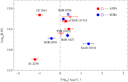
Figure 1: Log${}_{10}(t_{\rm SNR}/\tau_{\rm c})$ versus Log${}_{10}B$. The dot-dashed line corresponds to $t_{\rm SNR}=\tau_{\rm c}$. Blue circles and red squares represent SGRs and AXPs, respectively. Data for empty circles and squares are from Table 3. For some sources (e.g., SGR 1627), the errors in data-points are smaller than the size of the symbols.

In Fig. 1, magnetars with $n>3$ are on the left of the dashed line whereas those with $1<n<3$ are on the right. The large discrepancy between $t_{\rm SNR}$ and $\tau_{\rm c}$ of a magnetar can be naturally explained as follows: Inserting $P/\dot{P}=-\nu/\dot{\nu}=2\tau_{\rm c}$ into Eq. (10) gives $\tau_{\rm c}/t_{\rm SNR}=(n-1)/2$; if $n>3$, then $\tau_{\rm c}>t_{\rm SNR}$, and a magnetar looks “older” than its true age (e.g., 1E 1841). In this case, the larger the braking index is, the larger the disparity between $\tau_{\rm c}$ and $t_{\rm SNR}$, as illustrated by 1E 2259. If $1<n<3$, then $\tau_{\rm c}<t_{\rm SNR}$, and a magnetar appear “younger” than it is, the smaller the braking index is, the larger the age-disparity.

3.2 Case of $n>3$

The influence of the magnetic field evolution on the braking indices of radio-pulsars has been well investigated in previous studies (e.g., Geppert & Rheinhardt 2002; Aguilara et al. 2008; Pons & Geppert 2007; Pons et al. 2009; Viganò& Pons 2012; Viganò et al. 2012). In this subsection, we focus on three high braking indices ($n$=32$\pm$10, 13$\pm$4 and 6.3$\pm$1.7 for 1E 2259, 1E 1841 and SGR 0501, respectively). In order to explain why the three magnetars possess large braking indices, we consider the influences of crust magnetic field decay on a magnetar’s spin-down, and refer to the works of Pons et al (2009) and Viganò et al. (2013).

According to Pons et al.(2012), the spin evolution of an isolated NS is dominated by the magnetic field anchored to the star’s solid crust, and a varying crustal magnetic field yields the braking index

$$n=3-4\frac{\dot{B}_{\rm d}}{B_{\rm d}}\frac{\nu}{\dot{\nu}}=3-4\frac{\dot{B}_{\rm p}}{B_{\rm p}}\frac{\nu}{\dot{\nu}}=3-4\frac{\tau_{c}}{\tau_{B}},$$ (11)

where $B_{\rm d}$ is the surface dipole magnetic field, $B_{\rm p}=2B_{\rm d}$ is the surface magnetic field at the pole, and $\tau_{B}=B_{\rm p}/\dot{B_{\rm p}}=B_{\rm d}/\dot{B_{\rm d}}$ is the timescale on which the dipole component of the magnetic field evolves. From Eq.(11), a decreasing surface dipole magnetic field, $B_{\rm d}$, results in a decaying dipole braking torque, then the effective braking index increases to a high value of $n>3$.

In order to reconcile the measured high braking indices for three magnetars with their (estimated) surface field decaying-rates, it is necessary to introduce the Hall induction equation describing the evolution of crust magnetic field in the following form:

$$\frac{\partial\vec{B}}{\partial t}=-\nabla\times\left[\frac{c^{2}}{4\pi\sigma}\nabla\times(e^{\nu}\vec{B})+\frac{c}{4\pi en_{e}}[\nabla\times(e^{\nu}\vec{B})]\times\vec{B}\right],$$ (12)

where $\sigma$ is the electric conductivity parallel to the magnetic field, $e^{\nu}$ is the relativistic redshift correction, $n_{e}$ is the number of electrons per unit volume, and $e$ the electron charge. On the right-hand side, the first and second terms account for Ohmic dissipation and Hall effect (which redistributes the energy of the crustal magnetic field), respectively. As to the above differential equation, Aguilara et al. (2008) presented an analytic solution

$$\frac{dB_{\rm p}}{dt}=-\frac{B_{\rm p}}{\tau_{\rm Ohm}}-\frac{1}{B_{\rm p}^{i}}\frac{B_{\rm p}^{2}}{\tau_{\rm Hall}},$$ (13)

where $\tau_{\rm Ohm}$ is the Ohmic dissipation timescale, and $\tau_{\rm Hall}$ is the Hall timescale corresponding to an initial surface dipole magnetic field at the pole, $B_{\rm p}^{i}$. During a NS’s early magneto-thermal evolution stage, corresponding to the crust temperature $T\geq 10^{8}$ K, the average value of $\tau_{\rm Ohm}$ in the crust is about 1 Myrs (Pons & Gepport 2007). Since both the magnetic field strength and the density vary over many orders of magnitude in NSs’ crusts, the average Hall timescale is roughly restricted as $\tau_{\rm Hall}\sim\tau_{\rm Ohm}/(1-10)B_{13}$, where $B_{13}$ is the dipole magnetic field at the pole in units of $10^{13}$ Gauss (Pons & Gepport 2007). We choose $\tau_{\rm Hall}\sim 5\times 10^{2}-5\times 10^{5}$ yrs, similar as in Viganò et al. (2013), and $\tau_{\rm Ohm}\sim 10^{6}$ yrs for the three magnetars.

To estimate the values of $B_{\rm d}$ for the three magnetars, we refer to Viganò et al. (2013):

1. By introducing the state-of-the-art kinetic coefficients and considering the important effect of the Hall term, Viganò et al. (2013) presented the updated results of 2D simulations of the NS magneto-thermal evolution, and compared their results with a data sample of 40 sources including magnetars 1E 2259, 1E 1841 and SGR 0501. It was found that by only changing the initial magnetic fields, masses and envelope compositions of the NSs, the phenomenological diversity of magnetars, high-B radio-pulsars, and isolated nearby NSs can be well explained in their theoretical models.

2. These sources have best X-ray spectra by $Chandra$ or $XMM$-$Newton$, from which the luminosities and temperatures can be obtained, their well-established associations, and known timing properties with the characteristic age and the alternative estimate for the age. Similar as in this work, Viganò et al. (2013) selected their SNRs’ ages $\tau_{k}$ as the actual age estimates for the three magnetars (for 1E 2259, 1E 1841 and SGR 0501, $\log\tau_{k}$ (yr) $\simeq 4.0-4.3$, $2.7-3.0$, and 4, respectively, corresponding to $\tau_{k}$ are 10$-$20, 0.5 $-$1.0, and 10 kyrs, respectively). For generality, the Hall evolution timescales for the crustal fields have been arbitrarily selected as $10^{3}$, $10^{4}$, $10^{5}$, and $5.0\times 10^{5}$ yrs, respectively (Viganò et al. 2013).

3. Comparing the cooling curves with iron envelopes for $B_{\rm p}^{i}=10^{15}$ Gauss, 1E 1841 and SGR 0501 could be born with even higher magnetic field of a few $10^{15}$ Gauss, which can provide a strong hard X-ray (20$-$200 keV) emission with a total luminosity $\sim 10^{36}$ erg s^-1 (Viganò et al. 2013).

4. Comparing the cooling curves for the group of NSs with $B_{\rm d}^{i}\sim 1-5\times 10^{14}$ Gauss suggests that 1E 2259 may be born with $B_{\rm p}^{i}\sim 3\times 10^{14}$ Gauss, needed to reconcile the observed timing properties and the persistent soft X-ray luminosity.

According to the above arguments, we assume $B_{p}^{i}=3.0\times 10^{15}$ Gauss for 1E 1841 and SGR 0501, and $B_{p}^{i}\sim 3\times 10^{14}$ Gauss for 1E 2259. Inserting the values of $B_{\rm p}^{i}$, $B_{\rm p}$, $\tau_{\rm Ohm}$, and $\tau_{\rm Hall}$ into Eq.(13), we can obtain the estimated values of the surface magnetic field decay-rates $dB_{\rm p}/dt$. By solving Eq.(13), we obtain the relation of $dB_{\rm p}/dt$ and the field evolution timescale $t$ for the three magnetars, as shown in Fig. 2.

  

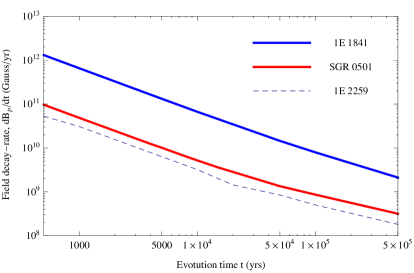
Figure 2: The relation of $dB_{\rm p}/dt$ and $t$ for three magnetars with $n>3$. The initial values of $B_{\rm p}$ are $1.4\times 10^{15}$, $3.8\times 10^{14}$, and $1.18\times 10^{14}$ Gauss for 1E 1841, SGR 0501, and 1E 2259, respectively.

From Fig.2, $dB_{\rm p}/dt$ decreases with increasing $t$. Due to the smallest value of $dB_{\rm p}^{i}$, the values of $B_{\rm p}/dt$ for 1E 2259 are lower than those of the other two magnetars. Assuming $t=\tau_{k}$ (Viganò et al. 2013), the current values of $dB_{\rm p}/dt$ of three magnetars are calculated as follows: $dB_{\rm p}/dt=-(1.32\times 10^{12}-6.55\times 10^{11}$ Gauss yr^-1 for 1E 1841, $dB_{\rm p}/dt=-(5.19\times 10^{9}$ Gauss yr^-1 for SGR 0501, and $dB_{\rm p}/dt=-(4.76\times 10^{9}-2.44\times 10^{9}$ Gauss yr^-1 for 1E 2259. SGR 0501 has the largest value of $dB_{\rm p}/dt$ because it has the smallest age $t=\tau_{k}=0.5-1.0$ kyrs. Thus, the values of timescale $\tau_{B}=B_{\rm p}/\dot{B_{\rm p}}$ can also be estimated as follows: for 1E 1841, $\tau_{B}=1.07-2.14$ kyrs, corresponding to $t=\tau_{k}=0.5-1.0$ kyrs, for SGR 0501, $\tau_{B}=73.2$ kyrs, corresponding to $t=\tau_{k}=10.0$ kyrs, and for 1E 2259, $\tau_{B}=24.8-48.4$ kyrs, corresponding to $t=\tau_{k}=10.0-20.0$ kyrs.

Assuming the surface dipolar field decay is the only factor influencing magnetar braking indices, by combining the values of $dB_{\rm p}/dt$ with Eq.(11), we plot the diagrams of $n$ versus $\log t$ for three magnetars, shown as in Fig.3.

  

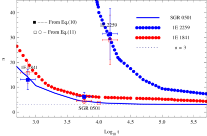
Figure 3: The relation of $n$ and $t$ for three magnetars with $n>3$.

In Fig.3, the solid-squares denote the values of $n$ obtained from Eq.(10) , and the empty-squares denote the values of $n$ obtained from Eq.(11) and the age-values presented in Viganò et al. (2013). The detailed calculations and comparisons are as follows:

1. For 1E 1841, when $t=\tau_{k}=0.5-1.0$ kyrs, which is consistent with the SNR age estimated by this work, its braking index $n=11.6-20.2$, which is comparable to the measured value of $n\sim$9$-$17 (see Table 4) in the magnitude.

2. For 1E 2259, when $t=\tau_{k}=10.0-20.0$ kyrs, which is also consistent with the SNR age estimated by this work, its braking index $n$=20$-$40, which approaches to the measured value of $n\sim$ 22$-$42 (see Table 4) in the magnitude.

3. For SGR 0501, when $t=\tau_{k}=10.0$ kyrs, its braking index $n=$3.8, which is apparently smaller than the measured value of $n\sim$ 4.6$-$8.0 (see Table 4). This discrepancy may be caused by: 1) the in1tial dipolar magnetic field estimated is too low; 2) the age estimate is too large (compared with $t=t_{SNR}=4.0-7.7$ kyrs in this work), and 3)the decay of the magnetospheric braking torque, e.g., the surface dipolar field decay cannot be the only factor influencing magnetar braking indices. Here, we insert $t=t_{SNR}=4.0-7.7$ kyrs into Eq.(11), then get $n\sim$4.1$-$5.0 (as denoted in the empty-circle in Fig.3), which is slightly larger than the value of $n=$3.8 by Viganò et al.(2013).

Although we have attributed the high-value braking indices of the three magnetars to the decay of the crustal surface magnetic field, there is the possibility of the decay of the magnetospheric braking torque, which can also result in the braking indices $n>3$. Below we will discuss the spin-down evolution for the three sources.

SGR 0501 was firstly discovered by the Swift $\gamma$-ray observatory (Barthelmy et al. 2008). From the RXTE/PCA, Swift/XRT, Chandra/ACIS-S, and XMM-Newton/PN observations spanning a short range of MJD 54700$-$54950, its magnitude of $\dot{\nu}$ decreased from $-2.03(8)\times 10^{-13}$ to $-1.75(6)\times 10^{-13}$ Hz s^-1 (Göǧüş et al., 2008, 2010). If this decrease in $\dot{\nu}$ is solely caused by the decay of $B_{\rm p}$, the mean surface dipolar field decaying-rate of $dB_{\rm p}/dt$ is $-(4.6\pm 0.8)\times 10^{13}$ Gauss yr^-1 (for a rotator in vacuum, $B_{\rm p}\simeq 6.4\times 10^{32}(-\dot{\nu}/\nu^{3})^{1/2}$ Gauss), corresponding to the braking index $n\sim 63.1-88.3$ obtained from Eq.(11).

Recently, Dib & Kaspi (2014) presented a summary of the long-term evolution of various properties of five AXPs including 1E 1841 and 1E 2259, regularly monitored with RXTE from 1996 to 2012. Influenced by frequent glitches and magnetar outbursts, 1E 1841 and 1E 2259 exhibited large fluctuations in their spin-down parameters $\nu$ and $\dot{\nu}$. However, both AXPs obviously exhibited net decrease in $\dot{\nu}$. For 1E 2259, its $\dot{\nu}$ decreased from $-1.020(17)\times 10^{-14}$ to $-0.96748\times 10^{-14}$ Hz s^-1 during an interval of MJD 50355$-$54852(Dib & Kaspi, 2014), which corresponds to $n\sim 1404.2-2653.8$ according to Eq.(11). For 1E 1841, its $\dot{\nu}$ decreased from $-2.9954(7)\times 10^{-14}$ to $-2.944(11)\times 10^{-13}$ Hz s^-1 during a interval of MJD 51225$-$55903(Dib & Kaspi, 2014), which corresponds to $n\sim 9.8-15.6$.

From the analysis above, apart from 1E 1841, the estimated values of $n$ from the surface dipolar magnetic field decay are far larger than the values of the measured mean braking indices for magnetars 1E 2259 and SGR 0501. We suppose that these large and rapid decreases in $\dot{\nu}$ were explained as the effects of timing-noise torque and outbursts (Göǧüş et al., 2010), instead of as a secular dipole magnetic field decay. An actual decay of magnetospheric torque may explain the high braking index for a magnetar, but could result in an over-estimate of the surface dipolar field decay rate.

Many authors (e.g., Harding et al 1999; Spitkovsky 2006; Beskin & Nokhrina 2007; Tasng & Gourgouliatos 2013; Antonopoulou et al. 2015) investigated the external magnetospheric mechanisms that can explain larger decrease in $|\dot{\nu}|$ during the pulsar spin-down. The rotation of a pulsar induces an electric field accelerating charges off the star’s surface. The magnetosphere is expected to be filled with cascade plasma, which will screen the electric field along the magnetic field lines (Goldreich & Julian 1969). The magnetospheric current, $\vec{J}$, flowing in the magnetosphere and closing under the polar-cap surface, provides an additional braking torque,

$$-\vec{T}_{\rm j}=\frac{1}{c}\int[\vec{r},[\vec{J}_{s},\vec{B}_{\rm p}]]dS~{}.$$ (14)

This braking torque on the star from the magnetospheric current is comparable to $-T_{\rm MDR}$, the braking torque on the star for MDR model From Eq. (14), a decreasing magnetospheric current $\vec{J}$ produces a decaying $-\vec{T}_{\rm j}$, which will cause a decrease in $\dot{\nu}$. For an net decay of toque due to the decrease in $\vec{J}$, the relative decrease in the spin-down rate is estimated as $\Delta T_{\rm j}/T_{\rm j}\simeq\Delta\dot{\Omega}/\dot{\Omega}=\Delta\dot{\nu}/\dot{\nu}$ assuming the momentum of inertial $I$, and the angle between rotational and magnetic axes, $\chi$ are constants. Note that, a precise calculation of $\dot{\Omega}$ (or $\dot{\nu}$) depends on solving the Euler dynamics equations that are very complicate and uncertain (Beskin & Nokhrina 2007).

It is also possible that a decrease in $\chi$ can cause a decrease in spin-down rate, as observed. During the long-term observations, these three magnetars with SNRs experienced frequent outbursts and glitches. (Göǧüş et al., 2008, 2010; Dib & Kaspi, 2014). During post-outburst or glitch recoveries, the stellar platelets move towards the rotational axes. The magnetic field lines anchored to the crusts follow the motion,and the inclination angle $\chi$ decreases (Antonopoulou et al. 2015). A decrease in $\chi$ will result in a net decay of the magnetospheric braking toque. Thus, the overall effect can be a decrease in $\dot{\nu}$. For a small decrease of $\chi$, the relative decrease in $\dot{\nu}$ is estimated as $\Delta T_{\rm dip}/T_{\rm MDR}\simeq\Delta\chi/{\rm tan}\chi\simeq\Delta\dot{\nu}/\dot{\nu}$ in MDR model, or as $\Delta T_{\rm ff}/T_{\rm ff}\simeq\Delta\chi{\rm\sin}2\chi/(1+{\rm\sin}^{2}\chi)\simeq\Delta\dot{\nu}/\dot{\nu}$, here $T_{\rm ff}$ is the braking torque for the force-free magnetosphere(Spitkovsky 2006; Antonopoulou et al. 2015). If the external magnetospheric mechanisms (whether due to the change in the current or due to the change in the inclination angle) dominate the spin-down evolutions for three magnetars, the order of magnitude of the relative decreases in the braking torque is about $|\Delta T/T|\approx|\Delta\dot{\nu}/\dot{\nu}|\sim 10^{-1}-10^{-2}$, as observed in 1E 2259, 1E 1841 and SGR 0501.

In summary, we have quantitatively analyzed several physical processes (the decay of surface dipolar field, the decline of the current, and the decrease in the inclination angle), possibly causing $n>3$ for magnetars. A common characteristic of these processes is that they can result in a decay of the braking torque on the star. Here we ignore the effects of the stellar multipole magnetic moments on the magnetar braking indices, because the higher-order magnetic moments decay rapidly with the distance to stellar center.

3.3 Case of $1<n<3$

In previous works, many authors proposed various models to explain why the observed braking indices of pulsars $1<n<3$, e.g., neutrino and photon radiation (Peng et al., 1982); the combination of dipole radiation and the propeller torque applied by debris-disk (Alpar & Baykal, 2006; Chen & Li, 2006); frequent glitches, as well as magnetosphere currents (Beskin & Nokhrina 2007). In this work, the lower braking indices of $1<n<3$ for five magnetars with SNRs are attributed to the combination of MDR and wind-aided braking. Recently, the extended emission observed from 1E 1547 and Swift J1834 are proposed to be magnetism-powered pulsar-wind-nebulas (PWNs), which may accelerate plasma to very high energy and radiate high-energy photons (see Kargaltsev et al. 2012, and references therein). The possible existence of magnetar PWNs lends a potential and direct support to our assumption of wind-aided braking.

With the aid of strong magnetar wind, the closed magnetic-field lines are combed out at the extended Alfvén radius $r_{\rm A}$, where the magnetic energy density equals the particle kinetic-energy density. The braking toque resulting from tangential acceleration of outflowing relativistic plasma is $-T_{\rm wind}\approx\dot{M}\Omega r^{2}_{\rm A}$, where $\dot{M}$ is the total mass-loss rate(Manchester et al., 1985). The accelerated outflowing plasma will carry away the star’s angular momentum, and thus the spin-down rate of the magnetar will increase. The added braking toque due to a magnetar wind extends the effective magnetic braking “lever arm ”, causing the magnetar braking index to decrease, i.e., $n<3$.

In the scenario of wind-aided braking, the value of the effective braking index $n$ of a magnetar depends on the competition of the magneto-dipole braking toque $-T_{\rm dip}$ and wind-braking toque $-T_{\rm wind}$. If $|T_{\rm wind}|\gg|T_{\rm dip}|$, the value of $n$ will be close to 1, and if $|T_{\rm dip}|\gg|T_{\rm wind}|$, the value of $n$ will be close to 3. Unlike the persistent soft X-ray luminosity of a magnetar $L_{\rm X}$, the persistent magnetar wind luminosity $L_{\rm W}$ cannot be obtained from observations. Moreover, it’s very difficult to determine $L_{\rm W}$ of a magnetar theoretically, due to the lack of a detailed magnetar-wind mechanism. The well-known magnetar wind-braking model proposed by Harding et al. (1999) implies a braking index of

$$n=~{}3-~{}\frac{2\nu}{\mid\dot{\nu}\mid}\frac{L_{\rm W}^{1/2}B_{\rm d}R^{3}}{2I\sqrt{6c^{3}}}~{},$$ (15)

where we employ standard values of $R=10\rm km$ and moment of inertia $I=10^{45}$ g cm². Note that, by definition, the inferred value of $n$ is always within the range of 1$-$3. In the above expression, $n$ is an effective braking index, thus $L_{\rm W}$ is the effective wind-luminosity, and $B_{\rm d}$ is the effective surface dipolar field. However, due to lack of the detailed information of the effective $n$, $B_{\rm d}$ and $L_{\rm W}$, the importance of Eq.(15) has not been recognized in previous works. From the above expression, the magnetar wind luminosity can be estimated as

$$L_{\rm W}=\frac{6(3-n)^{2}\dot{\nu}^{2}I^{2}c^{3}}{\nu^{2}B_{\rm d}^{2}R^{6}}.$$ (16)

By using Eq.(16), we estimated possible wind luminosity of magnetars, $L_{\rm W}$, as listed in Table 5. Here we assume that the effective value of surface dipolar field to be the observed value of $B_{\rm d}$ for convenience.

Table 5: The relations among $L_{\rm rot}$, $L_{\rm X}$ and $L_{\rm W}$ of magnetars with different braking indices. Five sources in the upper part of Table 5 have braking indices $1<n<3$, while three sources in the lower part have braking indices $n>3$. All the date $L_{\rm X}$(2-10 keV) in quiescence are cited from McGill SGR/AXP Online Catalogue.

Name	$L_{\rm rot}$	$L_{\rm X}$	$L_{\rm W}$	$L_{\rm W}/L_{\rm rot}$	$L_{\rm W}/L_{\rm X}$	$L_{\rm X}/L_{\rm rot}$
	($\rm erg~{}s^{-1}$)	($\rm erg~{}s^{-1}$)	($\rm erg~{}s^{-1}$)
SGR 1627∗	$4.3(9)\times 10^{34}$	$3.6\times 10^{33}$	(2.304$\pm$0.997)$\times 10^{35}$	5.36$\pm$2.58	64.0$\pm$27.7	0.08$\pm$0.02
Swift J1834∗	$2.1\times 10^{34}$	$<$ 0.84$\times 10^{31}$	(3.16$\pm$0.17)$\times 10^{35}$	15.03$\pm$0.78	37583.3$\pm$1964.3	$<$0.0004
CXOU J1714	$4.51\times 10^{34}$	$5.6\times 10^{34}$	(1.53$\pm$1.52)$\times 10^{35}$	3.39$\pm$3.37	2.73$\pm$2.71	1.242
$---^{{\dagger}}$	4.15$\times 10^{34}$	5.6$\times 10^{34}$	(1.15$\pm$1.57)$\times 10^{35}$	2.77$\pm$3.78	2.05$\pm$2.80	1.35
$---^{{\dagger}}$	7.41(35)$\times 10^{34}$	5.6$\times 10^{34}$	(5.36$\pm$4.26)$\times 10^{35}$	7.23$\pm$5.76	9.57$\pm$7.61	0.76$\pm$0.04
SGR 0526	2.87(7)$\times 10^{33}$	$1.89\times 10^{35}$	(4.13$\pm$0.55) $\times 10^{33}$	1.44$\pm$0.19	0.002$\pm$0.003	65.85$\pm$1.61
$---^{{\dagger}}$	4.9(4)$\times 10^{33}$	1.89$\times 10^{35}$	(2.75$\pm$0.53)$\times 10^{34}$	5.61$\pm$1.18	0.146$\pm$0.028	38.57$\pm$3.15
PSR J1622	8.3(5)$\times 10^{33}$	$4.4\times 10^{32}$	(1.47$\pm$0.40)$\times 10^{34}$	$1.77\pm$0.49	33.41$\pm$9.09	0.053$\pm$0.003
$---^{{\dagger}}$	(7.0$\pm$2.4)$\times 10^{33}$	4.4$\times 10^{32}$	(4.87$\pm$4.13)$\times 10^{33}$	0.69$\pm$0.58	11.1$\pm$9.4	0.063$\pm$0.022
1E 2259$+$586	$5.6\times 10^{31}$	$1.7\times 10^{34}$	…..	…..	…..	303.57
1E 1841$-$045	9.9$\times 10^{32}$	$1.84\times 10^{35}$	…..	…..	…..	185.85
SGR 0501$+$4516	$1.2\times 10^{33}$	$8.1\times 10^{32}$	…..	…..	…..	0.67

Footnote:^∗ According to the “fundamental plane”(Rea et al. 2012) for radio magnetars with $L_{\rm rot}>L_{\rm X}$, this source should have radio emission, however no radio emission was reported to date.

The rotation-energy loss rate is defined as $L_{\rm rot}=I\Omega\dot{\Omega}=4\pi^{2}I\nu\dot{\nu}=-4\pi^{2}I\dot{P}P^{-3}$, here $I=10^{45}$ g cm² for all sources. From Table 5, the value of $L_{\rm X}$ is obviously unrelated to that of $L_{\rm rot}$, this is because magnetar X-ray emission is powered by magnetic field free energy. With the exception of SGR 0526, magnetars’ wind luminosities are bigger than their soft X-ray luminosities. In addition, 1E 2259 possesses a relatively large ratio of $L_{\rm X}/L_{\rm rot}\sim 303.57$ (see in Table 5), which is higher than those of all magnetars. The large ratio of $L_{\rm X}/L_{\rm rot}$ could be served as a strong hint of surface dipolar field decay for this source, as discussed in Sec.3.2.

Recently, Tong et al. (2013) proposed a multipole field-powered wind model for magnetars. The authors assumed that all the high luminosity magnetars with $L_{\rm X}>L_{\rm rot}$ spin down via wind braking, and transient magnetars with $L_{\rm X}<L_{\rm rot}$ spin down via magnetic dipole braking. Based on a simple assumption of $L_{\rm W}=L_{\rm P}=10^{35}\,\rm erg\,s^{-1}$ ($L_{\rm P}$ is the escaping particle luminosity). They concluded that, for typical AXPs and SGRs, the dipole magnetic field in the case of wind braking is about ten-times lower than that of magnetic- dipole braking, and a strong dipole magnetic field may be no longer necessary for some sources and so on. However, when estimating $B_{\rm d}$, one should be cautious taking into account effective braking indices.

4 Summary and Discussion

Considering the possible SNR associations and their ages and assuming a constant braking index over the magnetar’s lives, we have estimated the average values of braking indices,for the eight magnetar, and discussed the possible origins of the braking indices. Our main conclusions are as follows.

1. Based on possible timing solutions of magnetars and updated measurements of their associated SNRs, we estimate the braking indices $n$ of eight magnetars, and find that they cluster in a range of $n\sim 1-42$.

2. We attribute the higher braking indices, $n>3$, of 1E 2259, 1E 1841 and SGR 0501 to the surface dipolar field decay, or to the decay of the external magnetospheric braking torque. In the former case, the estimated dipolar field decay rates, based on the updated magneto-thermal evolution models, are compatible with the measured values of $n$ for these three sources.

3. We attribute the lower mean braking indices, $1<n<3$, of other five magnetars (SGR 0526, SGR 1627, PSR J1622, CXOU J1714 and Swift J1734) to a combination of MDR and wind-aided braking, and estimate their possible wind luminosities $L_{\rm W}$.

At last, we remind that, in order to derive an analytical expression for estimating the magnetar’s true age, the braking index is assumed to be a constant. However, the inferred quantities (e.g., $B_{\rm d}$ and $\tau_{\rm c}$) of a magnetar strongly depend on the current values of $P$ and $\dot{P}$ (or of $\nu$ and $\dot{\nu}$) that can vary with time. There always exist observational errors when estimating $t_{\rm SNR}$ for magnetars. Thus, for some sources, their constrained values of $n$ are subject to substantial uncertainties, and will be modified with future observations. We expect that more observations of magnetars and their SNRs will help in further constraining the magnetar braking mechanisms.

References

- Aguilera et al. (2008) Aguilera D. N., et al., 2008, A& A, 486, 255
- Aharonian et al. (2008) Aharonian F., et al., 2008, A& A, 486, 829
- Alpar & Baykal (2006) Alpar M. A., Baykal A., 2006, MNRAS, 372, 489
- Anderson et al. (2012) Anderson G. E., et al., 2012, ApJ, 751, 53
- Antonopoulou et al. (2015) Antonopoulou D., et al., 2015, MNRAS, 447, 3924
- Archibald et al. (2014) Archibald R. F., et al., 2014, arXiv.1412.2789
- Badenes et al. (2009) Badenes C., et al., 2009, ApJ, 700, 727
- Bandiera (1984) Bandiera R., 1984, A& A, 139, 368
- Barsukov & Tsygan (2010) Barsukov D. P., Tsygan A. I., 2010, MNRAS, 409, 1077
- Barthelmy et al. (2008) Barthelmy S. D., et al., 2008, GCN Circ, 8113, 1
- Beskin & Nokhrina (2007) Beskin V. S., Nokhrina E. E., 2007, ApSS, 308, 569
- Biryukov et al. (2012) Biryukov A., et al., 2012, MNRAS, 420, 103
- Blandford & Romani (1988) Blandford R. D., Romani R. W., 1988, MNRAS, 234, 1988
- Camilo et al. (2008) Camilo F., et al., 2008, ApJ, 679, 681
- Castro et al. (2012) Castro D., et al. 2012, ApJ, 756, 88
- Caswell et al. (1975) Caswell J. L., et al. 1975, A&A, 45, 239
- Chen & Li (2006) Chen W. C., Li X. D., 2006, A&A, 450, L1
- Cioffi & et al. (1988) Cioffi D. F., et al., 1988, ApJ, 334, 252
- Clark & Stephenson (1975) Clark, D. H., Stephenson, F. R., 1975, The Observatory, 95, 190
- Corbel et al. (1999) Corbel S., et al., 1999, ApJ, 526, L29
- Cox (1972) Cox D., 1972, ApJ, 178, 159
- Downes et al. (1984) Downes A., et al., 1984, MNRAS, 210, 845
- Dib & Kaspi (2014) Dib R., Kaspi V. M., 2014, ApJ, 784, 37
- Duncan & Thompson (1992) Duncan R. C., Thompson C., 1992, ApJ, 392, L9
- Durant & van Kerkwijk (2006) Durant M., van Kerkwijk M H., 2006, ApJ, 650, 1070
- Ellison et al. (2007) Ellison D. C., et al., 2007, ApJ, 661, 879
- Esposito et al. (2009a) Esposito P., et al., 2009a, ApJ, 690, L105
- Espinoza et al. (2009b) Esposito P., et al., 2009b, MNRAS, 399, L44
- Espinoza et al. (2011) Espinoza C. M., et al., 2011, ApJ, 741, L13
- Espinoza (2013) Espinoza C. M., 2013, IAU Symposium, Vol.291, p.195, ed: J. van Leeuwen (Cambridge University Press)
- Evans et al. (1980) Evans W. D., et al., 1980, ApJ, 237, L7
- Fahlman & Gregory (1981) Fahlman G. G., Gregory P. C., 1981, Nature, 293, 202
- Ferdman et al. (2015) Ferdman R. D., et al., 2015, ApJ (submitted) arXiv:150600182
- Gaensler et al. (1999) Gaensler B. M., et al., 1999, ApJ, 526, L37
- Gaensler et al. (2001) Gaensler B. M., et al., 2001, ApJ, 559, 963
- Gaensler (2004) Gaensler B. M., 2004, Adv. Space. Res. 33, 645
- Gaensler & Slane (2006) Gaensler B. M., & Slane P. O., 2006, Annu. Rev. Astro. Astrophys. 44, 14
- Gaensler & Chatterjee (2008) Gaensler B. M., Chatterjee S., 2008, GCN Circ, 4189, 1
- Gaensler (2014) Gaensler B. M., 2014, GCN Circ, 16533, 1
- Geppert &Rheinhardt (2002) Geppert P., Rheinhardt M., 2002, A& A, 392, 1015
- Gao et al. (2011) Gao Z. F., et al. 2011, Ap&SS, 332, 129
- Gao et al. (2012) Gao Z. F., et al., 2012, Chin. Phy. B 21(5), 057109
- Gao et al. (2013) Gao Z. F., et al., 2013, Mod. Phys. Lett. A, 28(36), 1350138
- Gelfand & Gaensler (2007) Gelfand J. D., Gaensler B. M., 2007, ApJ, 667, 1111
- Gourgouliatos & Cumming (2015) Gourgouliatos K. N., Cumming A., 2015, MNRAS, 446, 1121
- Göǧüş et al. (2008) Göǧüş E., et al., 2008, ATel, 1677, 1
- Göǧüş et al. (2010) Göǧüş E., et al., 2010, ApJ, 722, 899, arXiv:1008.4089
- Goldreich&Julian (1969) Goldreich P., Julian W. H., 1969, ApJ, 157, 869
- Gotthelf&Vasisht (1997) Gotthelf E. V., Vasisht G., 1997, ApJ, 486, L133
- Halfand et al. (1994) Halfand D. J., et al., 1994, ApJ, 434, 627
- Halpern& Gotthelf (2010a) Halpern J. P., Gotthelf E. V., 2010a, ApJ, 710, 941
- Halpern& Gotthelf (2010) Halpern J. P.,Gotthelf E. V.,2010b,ApJ,725,1384
- Harding et al. (1999) Harding A. K., et al., 1999, ApJ, 525, L125
- Haskell & Melatos (2015) Haskell B., Melatos A., 2015, Int. J. Mod. Phys.D 24, 153008
- Ho (2011) Ho W. C. G., 2011, MNRAS. 414, 2567
- Hobbs et al. (2010) Hobbs G., et al., 2010, MNRAS, 402, 1027
- Horvath & Allen (2011) Horvath J. E., Allen M. D., 2011, RAA, 11, 625
- Hurley et al. (1999) Hurley K., et al., 1999, ApJ, 510, L107
- Kargaltsev et al. (2012) Kargaltsev O., et al., 2012, ApJ, 748, 26
- Klose et al. (2004) Klose S., et al., 2004, ApJ, 609, L13
- Kothes et al. (2002) Kothes R., et al., 2002, ApJ, 576, 169
- Kothes & Foster (2012) Kothes R., Foster T., 2012, ApJ, 746, L4
- Kou & Tong (2015) Kou F F., Tong H., 2015, MNRAS, 450, 1990
- Kouveliotou et al. (1994) Kouveliotou C., et al., 1994, Nature, 368, 125
- Kutukcu & Ankay (2014) Kutukcu P., Ankay A., 2014, Int. J.Phys.D. 23, 1450083
- Kulkarni et al. (2003) Kulkarni S. R., et al., 2003, ApJ, 585, 948
- Lai et al. (2013) Lai X. Y., Gao C. Y., Xu R. X., 2013, MNRAS, 431, 3282
- Leahy & Aschenbach (1995) Leahy D. A., Aschenbach B., 1995, A& A, 293, 853
- Leahy & Tian (2007) Leahy D. A., Tian W. W., 2007, A& A, 461, 1013
- Levin et al. (2010) Levin L., et al., 2010, ApJ, 721, L33
- Livingstone et al. (2007) Livingstone M. A., et al., 2007, ApSS, 308, 317
- Lyne et al. (1993) Lyne A. G., et al., 1993, MNRAS, 265, 1003
- Magalhaes et al. (2012) Magalhaes N. S., et al., 2012, ApJ, 755, 54
- Manchester & Taylor (1977) Manchester R. N., Taylor J. H., 1977, Pulsars (W. H. Freeman & Co Ltd)
- Manchester et al. (1985) Manchester R. N., et al., 1985, Nature, 313, 374
- Manchester et al. (2005) Manchester R. N., et al., 2005, AJ, 129, 1993
- Martin et al. (2014) Martin J., et al., 2014, MNRAS, 444, 2910
- Mereghetti (2008) Mereghetti S., 2008, Astron. Astrophys. Rev. 15, 225
- Middleditch et al. (2006) Middleditch J., et al., 2006, ApJ, 652, 1531
- Muslimov & Page (1995) Muslimov A., Page D., 1995, ApJ, 440, L77
- Nakamura et al. (2009) Nakamura R., et al., 2009, PASJ, 61, S197
- Olausen & Kaspi (2014) Olausen S. A., Kaspi V. M., 2014, ApJS, 212, 6
- Ostriker & McKee (1988) Ostriker J.P., McKee C.F., 1988, Rev. Mod. Phy. 60, 1
- Park et al. (2012) Park S., et al., 2012, ApJ, 748, 117
- Peng et al. (1982) Peng Q. H., et al., 1982, A&A, 107, 258
- Pons & Geppert (2007) Pons J. A., Geppert U., 2007, A& A, 470, 303
- Pons et al. (2009) Pons J. A., Miralles J. A., Geppert U., 2007, A&A, 496, 207
- Pons et al. (2012) Pons J. A., Viganò D., Geppert U., 2012, A&A, 547, A9
- Rea et al. (2012) Rea N., et al., 2012, ApJ, 748, L12
- Romer et al. (2001) Romer A. K., et al., 2001, ApJ, 547, 594
- Roy et al. (2012) Roy J., et al., 2012, MNRAS, 424, 2213
- Sarma et al. (1997) Sarma, A., et al., 1997, ApJ, 483, 335
- Sasaki et al. (2004) Sasaki M., et al., 2004, ApJ, 617, 322
- Sasaki et al. (2013) Sasaki M., et al., 2013, A& A, 552, 45
- Sato et al. (2010) Sato T., et al., 2010, PASJ, 62, L33
- Sedov (1946) Sedov L. I., 1946, Dokl. Akad. Nauk SSSR, 42, 17
- Sedov (1959) Sedov L. I., 1959, Similarity and Dimentional Methods in Mechanics, Academic Press, New York
- Smith et al. (1999) Smith D. A., et al., 1999, ApJ, 519, L147
- Spitkovsky (2006) Spitkovsky A., 2006, ApJ, 648, L51
- Taylor (1950) Taylor G., 1950, Proc.R.Soc. London. A, 201, 159
- Tendulkar et al. (2012) Tendulkar S. P., et al., 2012, ApJ,761, 76
- Thompson & Duncan (1996) Thompson C., Duncan R. C., 1996, ApJ, 473, 322
- Tian & Leahy (2008) Tian W. W., Leahy D. A., 2008, ApJ, 677, 292
- Tian & et al. (2007) Tian W. W., et al., 2007, ApJ, 657, L25
- Tian& et al. (2010) Tian W. W., et al., 2010, MNRAS, 404, L1
- Tian & Leahy (2012) Tian W. W., Leahy D. A., 2012, MNRAS, 421, 2593
- Tiengo et al. (2009) Tiengo A., et al., 2009, MNRAS, 399, L74
- Tong et al. (2013) Tong H., et al., 2013, ApJ, 768, 144
- Truelove & McKee (1999) Truelove J.K., McKee C.F., 1999, ApJS, 120, 299
- Vasisht & Gotthelf (1997) Vasisht G., Gotthelf E. V.,1997, ApJ, 486, L129
- Vink & Kuiper (2006) Vink J., Kuiper L., 2006, MNRAS, 370, L370
- Viganò& et al. (2012) Viganò D., Pons J. A., Miralles J. A., 2012, Computer Physics. Communications, 183, 2042
- Viganò& Pons (2012) Viganò D., Pons J. A., 2012, MNRAS, 425, 2487
- Viganò et al. (2013) Viganò D., Rea N., Pons J. A., et al., 2013, MNRAS, 434, 123
- Weltevrede et al. (2011) Weltevrede P., et al., 2011, MNRAS, 411, 1917
- White & Long (1991) White R., Long K., 1991, ApJ, 373, 543
- Woltjer (1972) Woltjer L., 1972, Anu. Rev. Astron. Astrophys. 10, 129
- Yan et al. (2015) Yan Z., Shen Z. Q., Wu X. J., et al. 2015. arxiv:1510.00183v1
- Yuan et al. (2010) Yuan J. P., et al., 2010, ApJ, 719, L111
- Xu (2007) Xu R. X., 2007, Advances in Space Research, 40, 1453
- Zhang & Xie (2012) Zhang S.-N., Xie Y., 2012, ApJ, 761, 102
- Zhang & Xie (2013) Zhang S.-N., Xie Y., 2013, Int. J. Mod. Phys.D., 22, 1360012
- Zheng et al. (2006) Zheng X. P., Yu Y. W., Li J. R., 2006, MNRAS, 369, 376
- Zhu et al. (2014) Zhu H., Tian,W. W., Zuo, P., 2014, ApJ, 793, 95