Gutzwiller Wave-Function Solution for Anderson Lattice Model:
Emerging Universal Regimes of Heavy Quasiparticle States

Abstract

The recently proposed diagrammatic expansion (DE) technique for the full Gutzwiller wave function (GWF) is applied to the Anderson lattice model. This approach allows for a systematic evaluation of the expectation values with full Gutzwiller wave function in the finite dimensional systems. It introduces results extending in an essential manner those obtained by means of standard Gutzwiller approximation (GA) scheme which is variationally exact only in infinite dimensions. Within the DE-GWF approach we discuss principal paramagnetic properties and their relevance to the heavy fermion systems. We demonstrate the formation of an effective, narrow $f$-band originating from atomic $f$-electron states and subsequently interpret this behavior as a direct itineracy of $f$-electrons; it represents a combined effect of both the hybridization and the correlations reduced by the Coulomb repulsive interaction. Such feature is absent on the level of GA which is equivalent to the zeroth order of our expansion. Formation of the hybridization- and electron-concentration-dependent narrow $f$-band rationalizes common assumption of such dispersion of $f$ levels in the phenomenological modeling of the band structure of CeCoIn₅. Moreover, it is shown that the emerging $f$-electron direct itineracy leads in a natural manner to three physically distinct regimes within a single model, that are frequently discussed for 4$f$- or 5$f$- electron compounds as separate model situations. We identify these regimes as: (i) mixed-valence regime, (ii) Kondo-insulator border regime, and (iii) Kondo-lattice limit when the $f$-electron occupancy is very close to the $f$-states half-filling, $\langle\hat{n}_{f}\rangle\rightarrow 1$. The nonstandard features of emerging correlated quantum liquid state are stressed.

I Introduction and Motivation

Heavy fermion systems (HFS) belong to the class of quantum materials with strongly correlated 4$f$ or 5$f$ electrons. They exhibit unique properties resulting from their universal electronic features (e.g. very high density of states at the Fermi level) almost independent of their crystal structure. Among those unique properties are: (i) enormous effective masses in the Fermi-liquid state, as demonstrated through the linear specific heat coefficient Andres et al. (1975); Stewart (1984); Grewe and Steglich (1991); Fulde et al. (1988); Ott (1987) and their direct spin-dependence in the de Haas-van Alphen measurements Citro et al. (1999); Sheikin et al. (2003); McCollam et al. (2005), (ii) Kondo-type screening of localized or almost localized $f$-electron magnetic moments by the conduction electrons Doradziński and Spałek (1997, 1998), (iii) unconventional superconductivity, appearing frequently at the border or coexisting with magnetism Pfleiderer (2009), and (iv) abundance of quantum critical points and associated with them non-Fermi (non-Landau) liquid behavior Stewart (2001); Löhneysen et al. (2007); Lonzarich (2005).

The Anderson lattice model (ALM), also frequently referred to as periodic Anderson model, and its derivatives: the KondoLacroix and Cyrot (1979); Hewson (1993); Auerbach and Levin (1987) and the Anderson-KondoHowczak and Spałek (2012); Howczak et al. (2013) lattice models, capture the essential physics of HFS. Although, the class of exact solutions is known for this modelGurin and Gulácsi (2001); Gulácsi (2002); Gulácsi and Vollhardt (2003, 2005), they are restricted in the parameter space. Thus, for thorough investigation of the model properties the approximate methods are needed. One of the earliest theoretical approaches for the models with a strong Coulomb repulsion was the variational Gutzwiller wave function (GWF) method Varma et al. (1986); Gulácsi et al. (1993a); Rice and Ueda (1985, 1986); Miyake et al. (1986); Fazekas (1999). However, despite its simple and physically transparent form, a direct analytic evaluation of the expectation values with full GWF cannot be carried out rigorously for arbitrary dimension and spatially unbound systems.

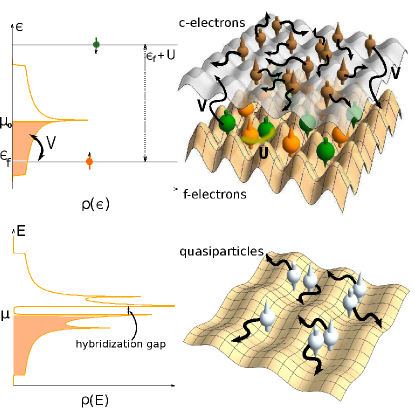
Figure 1: (Color online) Upper part: Schematic representation of the two-orbital Anderson lattice model with initially localized $f$- and delocalized $c$-electrons, and hybridization between them. Bottom part: Emerging quasiparticle states in the hybridized bands of correlated particles. On the left: the shapes of the density of states in the respective situations.

One of the ways of overcoming this difficulty is the so-called Gutzwiller Approximation (GA), in which only local two-particle correlations are taken into account when evaluating the expectation values. GA provides already a substantial insight into the overall properties of strongly correlated systems Rice and Ueda (1985); Kotliar and Ruckenstein (1986); Spałek et al. (1987); Gebhard (1991); Dorin and Schlottmann (1992, 1993); Doradziński and Spałek (1997, 1998); Bünemann et al. (1998). Moreover, this approach has been reformulated recently to the so-called statistically-consistent Gutzwiller approximation (SGA) scheme and successfully applied to a number of problems involving correlated electron systems Jȩdrak and Spałek (2011); Kaczmarczyk and Spałek (2011); Howczak et al. (2013); Abram et al. (2013); Ka̧dzielawa et al. (2013); Zegrodnik et al. (2014); Wysokiński and Spałek (2014); Wysokiński et al. (2014, 2015). Among those, a concrete application has been a microscopic description of the fairly complete magnetic phase diagram of UGe₂ Wysokiński et al. (2014, 2015) which provided quantitatively correct results, even without taking into account the 5$f$-orbital degeneracy due to uranium atoms.

An advanced method of evaluating the expectation values for GWF is the variational Monte Carlo technique (VMC) Edegger et al. (2006); Lugas et al. (2006); Raczkowski et al. (2007); Edegger et al. (2007); Chou et al. (2012); Liu et al. (2005); Watanabe et al. (2009); Asadzadeh et al. (2013); Watanabe et al. (2015). However, this method is computationally expensive and suffers from the system-size limitations. Though, one must note that the VMC method allows for extension of GWF by including e.g. Jastrow intersite factors Jastrow (1955).

Here we use an alternative method of evaluating the expectation values for GWF, namely a systematic diagrammatic expansion for the Gutzwiller wave function (DE-GWF) Bünemann et al. (2012); Kaczmarczyk et al. (2013, 2014); Kaczmarczyk (2015); Kaczmarczyk et al. (2015). This method was formulated initially for the Hubbard model in two dimensions in the context of Pomeranchuk instabilityBünemann et al. (2012), and applied subsequently to the description of high-temperature superconductivity for the HubbardKaczmarczyk et al. (2013, 2015) and the $t$-$J$Kaczmarczyk et al. (2014) models. In the zeroth order of the expansion this approach straightforwardly reduces to the GAKaczmarczyk et al. (2014). For the one-dimensional Hubbard model it converges Bünemann et al. (2012) to the exact GWF results. Within DE-GWF a larger variational space can be sampled than within the alternative VMC technique because the long-range components of the effective Hamiltonian are accounted for naturally. The DE-GWF method (truncated to match the variational spaces) reproduces the results of VMC with improved accuracy (as shown for the $t$-$J$ Kaczmarczyk et al. (2014) and the Hubbard models Kaczmarczyk et al. (2013)). Additionally, the method works also in the thermodynamic limit. In effect, the approach is well suited to capture subtle effects, e.g. those related to the topology of the Fermi surface in the correlated state Bünemann et al. (2012) or the investigated here formation of a narrow $f$-electron band.

In this study, we extend the DE-GWF approach to discuss principal paramagnetic properties within ALM. The emergence of the quasiparticle picture is schematically illustrated in Fig.1. Explicitly, we investigate the shape of the quasiparticle density of states (DOS, $\rho(E)$), evolving with the increasing order of the expansion, $k$. For $k>0$ the hybridization gap widens up with respect to that in GA ($k=0$ case) and DOS peaks are significantly pronounced. Moreover, we investigate the DOS at the Fermi level ($\rho(E_{F})$) evolution with the increasing the hybridization strength $|V|$ – total electron concentration $n$, plane, as it is a direct measure of the heavy-quasiparticle effective mass. We find that this parameter is significantly enhanced for $k>0$, mainly in the low hybridization limit and at the border of the Kondo-insulating state. Furthermore, we trace the contribution coming from the originally localized $f$-electrons (cf. Fig. 1 - upper part) to the quasiparticle spectrum with the increasing order of the expansion. For $k>0$, $f$-quasiparticles effectively acquire a nonzero bandwidth (up to 6% of the conduction bandwidth) as a combined effect of both interelectronic correlations and hybridization.

Assumption of a narrow $f$ band existence has recently been made in a phenomenological modeling of the heavy fermion compound CeCoIn₅ band structure Aynajian et al. (2012); Allan et al. (2013); Dyke et al. (2014). We show that the emergence of such a band, absent in GA ($k=0$), is an evidence of the $f$-electron direct itineracy explained later. To quantify this itineracy we introduce the parameter $w_{f}$ - the width of the effective, narrow $f$-band. On the hybridization strength – total electron concentration, $|V|$ – $n$ plane, $w_{f}$ is significantly enlarged in the three distinct regimes, which we identify respectively as the mixed-valence, Kondo/almost Kondo insulating, and the Kondo-lattice regimes (when $f$-electron concentration is close to the half-filling, i.e., when $\langle\hat{n}_{f}\rangle\rightarrow 1$). These physically distinct regimes are frequently discussed and identified in various experiments Holmes et al. (2004); Ślebarski and Spałek (2005); Pfleiderer (2009); Stewart (1984); Ślebarski et al. (2010); Szlawska et al. (2009); Kaczorowski and Ślebarski (2010) and in theory Watanabe and Miyake (2010); Howczak et al. (2013); Dorin and Schlottmann (1992); Tsunetsugu et al. (1997).

The structure of the paper is as follows. In Sec. II we describe the ALM Hamiltonian and define the Gutzwiller variational wave function in a nonstandard manner. In Sec. III we derive the DE-GWF method for ALM and determine the effective single-particle two-band Hamiltonian. In Sec. IV we present results concerning paramagnetic properties: the quasiparticle spectrum, the resultant density of states at the Fermi level, and formation of an effective narrow $f$-electron band out of initially localized states. In Appendix A we discuss the equivalence of the zeroth-order DE-GWF approach with GA. In Appendix B we present some technical details of DE-GWF technique.

II Model Hamiltonian and Gutzwiller wave function

Our starting point is the Anderson lattice model (ALM) with the chemical potential $\mu$ and expressed through Hamiltonian

$$\begin{gathered}\mathcal{\hat{H}}={\sum_{{\bf i},{\bf j},\sigma}}t_{{\bf i}{\bf j}}\hat{c}_{{\bf i}\sigma}^{\dagger}\hat{c}_{{\bf j}\sigma}-\sum_{{\bf i},\sigma}\mu\hat{n}^{c}_{{\bf i}\sigma}+\sum_{{\bf i},\sigma}(\epsilon_{f}-\mu)\hat{n}^{f}_{{\bf i}\sigma}\\ +U\sum_{\bf i}\hat{n}^{f}_{{\bf i}\uparrow}\hat{n}^{f}_{{\bf i}\downarrow}+\sum_{{\bf i},{\bf j},\sigma}(V_{{\bf i}{\bf j}}\hat{f}_{{\bf i}\sigma}^{\dagger}\hat{c}_{{\bf j}\sigma}+V^{*}_{{\bf i}{\bf j}}\hat{c}_{{\bf i}\sigma}^{\dagger}\hat{f}_{{\bf j}\sigma}),\end{gathered}$$ (1)

where ${\bf i}=(i_{x},i_{y})$ (and similarly ${\bf j}$) is the two-dimensional site index, $\hat{f}_{{\bf i}\sigma}$ ($\hat{f}^{\dagger}_{{\bf i}\sigma}$) and $\hat{c}_{{\bf i}\sigma}$ ($\hat{c}^{\dagger}_{{\bf i}\sigma}$) are the annihilation (creation) operators related to $f$- and $c$- orbitals respectively, and $\sigma=\uparrow,\downarrow$ is the $z$-component direction of the spin. We assume that the hopping in the conduction band takes place only between the nearest neighboring sites, $t_{{\bf i}{\bf j}}\equiv t\delta_{|{\bf i}-{\bf j}|,1}$, the hybridization has the simplest onsite character not , $V_{{\bf i}{\bf j}}=V\delta_{{\bf i},{\bf j}}$, the local Coulomb repulsion on the $f$ orbital has the amplitude $U$, and the initially atomic $f$ states are located at the energy $\epsilon_{f}$. In the following $|t|$ is used as the energy unit.

Gutzwiller wave function (GWF) is constructed from the uncorrelated Slater determinant $|\psi_{0}\rangle$ by projecting out fraction of the local double $f$-occupancies by means of the Gutzwiller projection operator $\hat{P}_{G}$,

$$|\psi_{G}\rangle\equiv\hat{P}_{G}|\psi_{0}\rangle\equiv\prod_{{\bf i}}\hat{P}_{G;{\bf i}}|\psi_{0}\rangle.$$ (2)

In the GA approach when only a single $f$ orbital (in the present case) is correlated the projection operator can be defined by

$$\hat{P}_{G;{\bf i}}\equiv 1-(1-g)\hat{n}_{{\bf i}\uparrow}^{f}\hat{n}_{{\bf i}\downarrow}^{f},$$ (3)

where $g$ is a variational parameter. Such form allows for interpolating between the fully correlated ($g=0$) and the uncorrelated ($g=1$) limits. Equivalently one can consider average number of doubly occupied states, $\langle\hat{n}_{{\bf i}\uparrow}^{f}\hat{n}_{{\bf i}\downarrow}^{f}\rangle\equiv d^{2}$ as a variational parameter.

The Gutzwiller projection operator can be selected differently as proposed in Ref. Gebhard, 1990, namely

$$\hat{P}_{G;{\bf i}}^{\dagger}\hat{P}_{G;{\bf i}}\equiv\hat{P}_{G;{\bf i}}^{2}={\bf 1}+x\hat{d}_{{\bf i}}^{HF}.$$ (4)

In the above relation $x$ is a variational parameter and for the paramagnetic and translationally invariant system we define Hartree-Fock (HF) operators of the form

$$\hat{d}_{{\bf i}}^{HF}\equiv\hat{n}^{HF}_{{\bf i}\uparrow}\hat{n}^{HF}_{{\bf i}\downarrow}=(\hat{n}_{{\bf i}\uparrow}^{f}-n_{0f})(\hat{n}_{{\bf i}\downarrow}^{f}-n_{0f}),$$ (5)

where $n_{0f}$ denotes average occupation of a single $f$ state and spin $\sigma$ in the uncorrelated state, $|\psi_{0}\rangle$, i.e., ${n_{0f}=\langle\hat{f}_{{\bf i}\sigma}^{\dagger}\hat{f}_{{\bf i}\sigma}\rangle_{0}}$. Hereafter the shortened notation for the expectation values is used, i.e., $\langle\psi_{0}|...|\psi_{0}\rangle\equiv\langle...\rangle_{0}$. Strictly speaking, although, $\hat{d}_{{\bf i}}^{HF}$ has not the Hartree-Fock form of the double occupancy operator, the HF superscript has its meaning as the property, $\langle\hat{d}_{{\bf i}}^{HF}\rangle_{0}\equiv 0$ is preserved.

On the other hand, the Gutzwiller projection operator can be defined in general form as

$$\hat{P}_{G;{\bf i}}=\sum_{\Gamma}\lambda_{\Gamma}\mid\Gamma\rangle_{{\bf i}}\langle\Gamma\mid_{{\bf i}},$$ (6)

with variational parameters $\lambda_{\Gamma}\in\{\lambda_{0},\lambda_{\uparrow},\lambda_{\downarrow},\lambda_{d}\}$ that characterize the possible occupation probabilities for the four possible atomic Fock $f$-states ${\mid\Gamma\rangle_{{\bf i}}\in\{\mid 0\rangle_{{\bf i}},\mid\uparrow\rangle_{{\bf i}},\mid\downarrow\rangle_{{\bf i}},\mid\uparrow\downarrow\rangle_{{\bf i}}\}}$.

Relation (4) couples $\lambda_{\Gamma}$ and $x$, reducing the number of independent variational parameters to one. Explicitly, we may express the parameters $\lambda_{\Gamma}$ by the coefficient $x$,

$$\begin{split}\lambda_{0}^{2}&=1+xn_{0f}^{2},\\ \lambda_{\sigma}^{2}=\lambda_{\bar{\sigma}}^{2}\equiv\lambda_{s}^{2}&=1-xn_{0f}(1-n_{0f}),\\ \lambda_{d}^{2}&=1+x(1-n_{0f})^{2}.\end{split}$$ (7)

As the parameters $\lambda_{\Gamma}$ and $x$ are coupled by the conditions (7), there is a freedom of choice of the variational parameter; in this work we have selected $x$. The parameter $x$ covers the same variational space as $g$ in GA. Additionally, the projector (4) leads to much faster convergence than (3) (cf. Ref. Bünemann et al., 2012). From (4) it is clear that $x=0$ corresponds to the uncorrelated limit. The other extremity, the fully correlated state is reached for $x=\max\{x(\lambda_{d}=0),x(\lambda_{0}=0)\}$. This leads to the bounds $\max\{\frac{-1}{(1-n_{0f})^{2}},\frac{-1}{(n_{0f})^{2}}\}\leq x\leq 0$. The minimal value is $x=-4$ for $n_{0f}=0.5$.

The method is suitable for an arbitrary filling of the $f$ orbital. However, due to the fact that present work is mainly addressed to the description of the Ce-based compounds, we study the regime in which the $f$-orbital filling either does not exceed unity or is only slightly larger. Precisely, in the all figures presented here the $f$-orbital filling is never larger than 1.05.

III DE-GWF Method

III.1 General scheme

In this section we present general implementation of the DE-GWF method. The procedure is composed of the following steps:

1. Choice of initial state $|\psi_{0}\rangle$.

2. Evaluation of $\langle\mathcal{\hat{H}}\rangle_{G}\equiv\frac{\langle\psi_{G}\mid\mathcal{\hat{H}}\mid\psi_{G}\rangle}{\langle\psi_{G}\mid\psi_{G}\rangle}$ for selected $|\psi_{0}\rangle$ - cf. Sec. III.2.

3. Minimization of $\langle\mathcal{\hat{H}}\rangle_{G}$ with respect to the variational parameter (here $x$).

4. Construction of the effective single particle Hamiltonian determined by $\delta\mathcal{\hat{H}}^{\rm eff}(|\psi_{0}\rangle)=\delta\mathcal{\hat{H}}(|\psi_{0}\rangle)$ - cf. Sec. III.3.

5. Determination of $|\psi^{\prime}_{0}\rangle$ as a ground state of the effective Hamiltonian - cf. Sec. III.4.

6. Execution of the self-consistent loop: starting again from the step 1 with $|\psi^{\prime}_{0}\rangle$ until a satisfactory convergence, i.e., $|\psi^{\prime}_{0}\rangle=|\psi_{0}\rangle$, is reached.

Steps 4 and 5 ensure that the final form of $|\psi_{0}\rangle$ represents the optimal choice which minimizes the ground state energy $\langle\mathcal{\hat{H}}\rangle_{G}$. The DE-GWF method with respect to other related methods, GA and VMC, introduces a new technique for evaluating the expectation value of the correlated Hamiltonian with GWF (step 2 of the above procedure). In particular, it provides an important improvement as, e.g., for GA only single sites in the lattice contain the projection whereas the remaining environment does not. GA leads e.g. to the inability of obtaining the superconducting phase in the Hubbard model Kaczmarczyk et al. (2013). On the other hand, the VMC method tackles that problem properly, but at the price of extremely large computing power needed. This leads to the lattice size limitations (typically up to 20x20 sites) and a limited distance of real space intersite correlations taken into account.

In this respect, DE-GWF introduces, in successive orders of the expansion, correlations to the environment of individual sites (beyond GA), as well as converges in a systematic manner to the full GWF solution. Also, DE-GWF was shown to provide results of better accuracy than VMC Kaczmarczyk et al. (2014), and additionally, is free from the finite-size limitations. It also demands definitely less computational power than VMC. Thus in general, this method is capable of treating more complex problems with GWF. On the other hand, DE-GWF is tailored specifically for GWF, while VMC allows for starting from different forms of variational wave function e.g., adding the Jastrow factorsJastrow (1955); Watanabe et al. (2015).

III.2 Diagrammatic expansion

The key point of the variational procedure is the calculation of the expectation value of Hamiltonian (1) with GWF $|\psi_{G}\rangle$ (point 1 from the scheme in Sec. III.1), by starting from the expression

$$\begin{gathered}\langle\mathcal{\hat{H}}\rangle_{G}\equiv\frac{\langle\psi_{G}\mid\mathcal{\hat{H}}\mid\psi_{G}\rangle}{\langle\psi_{G}\mid\psi_{G}\rangle}=\frac{\langle\psi_{0}\mid\hat{P}_{G}\mathcal{\hat{H}}\hat{P}_{G}\mid\psi_{0}\rangle}{\langle\psi_{0}\mid\hat{P}_{G}^{2}\mid\psi_{0}\rangle}.\end{gathered}$$ (8)

We use the DE-GWF technique Bünemann et al. (2012); Kaczmarczyk et al. (2013, 2014); Kaczmarczyk (2015), based on the expansion of the expectation values appearing in Eq. (8) in the power series in variational parameter $x$, with the highest power representing number of correlated vertices assumed to be correlated in the environment - besides local ones. This method is systematic in the sense that the zeroth order corresponds to GA Edegger et al. (2007), whereas with the increasing order the full GWF solution is approached. Explicitly, we determine expectation values with respect to GWF of any product operator originating from the starting Hamiltonian (1) ${{\mathcal{\hat{O}}_{{\bf i}({\bf j})}}=\{\hat{c}_{{\bf i}\sigma}^{\dagger}\hat{c}_{{\bf j}\sigma},\hat{n}^{c}_{{\bf i}\sigma},\hat{n}^{f}_{{\bf i}\sigma},\hat{n}^{f}_{{\bf i}\uparrow}\hat{n}^{f}_{{\bf i}\downarrow},\hat{f}_{{\bf i}\sigma}^{\dagger}\hat{c}_{{\bf j}\sigma},\hat{c}_{{\bf i}\sigma}^{\dagger}\hat{f}_{{\bf j}\sigma}\}}$. This is executed by first accounting for the projection part on the site ${\bf i}({\bf j})$ - external vertices (e.g., computing ${{\hat{\mathcal{O}}^{G}_{{\bf i}({\bf j})}}\equiv\hat{P}_{G;{\bf i}}(\hat{P}_{G;{\bf j}})\hat{\mathcal{O}}_{{\bf i}({\bf j})}(\hat{P}_{G;{\bf j}})\hat{P}_{G;{\bf i}}}$, see below) and then, including one-by-one correlations (terms) to the other sites ${\bf l}\neq{\bf i},{\bf j}$ - internal vertices.

Formally, the procedure starts in effective power expansion in $x$ of all relevant expectation values

$$\begin{gathered}\langle\psi_{G}\mid\hat{\mathcal{O}}_{{\bf i}({\bf j})}\mid\psi_{G}\rangle=\Big{\langle}\hat{{\mathcal{O}}}^{G}_{{\bf i}({\bf j})}\prod_{{\bf l}\neq{\bf i},{\bf j}}\hat{P}_{G;l}^{2}\Big{\rangle}_{0}\\ =\sum_{k=0}^{\infty}\frac{x^{k}}{k!}{\sum_{{\bf l}_{1},...,{\bf l}_{k}}}^{\prime}\langle\hat{{\mathcal{O}}}^{G}_{{\bf i}({\bf j})}\hat{d}^{HF}_{{\bf l}_{1},...,{\bf l}_{k}}\rangle_{0},\end{gathered}$$ (9)

where $\hat{d}^{HF}_{{\bf l}_{1},...,{\bf l}_{k}}\equiv\hat{d}^{HF}_{{\bf l}_{1}}\cdots\hat{d}^{HF}_{{\bf l}_{k}}$. The prime in the multiple summation denotes restrictions: ${\bf l}_{p}\neq{\bf l}_{p^{\prime}}$, and ${\bf l}_{p}\neq{\bf i},{\bf j}$ for all $p,p^{\prime}$. $k$ is the order of the expansion. Note that for $k=0$ we obtain $\langle\psi_{G}|\hat{\mathcal{O}}_{{\bf i}({\bf j})}|\psi_{G}\rangle=\langle\hat{{\mathcal{O}}}^{G}_{{\bf i}({\bf j})}\rangle_{0}$. This means that the projection operators act only locally (i.e., only the sites ${\bf i}$ and ${\bf j}$ are affected) and in this case we recover the GA results (for a details discussion of the equivalence see Appendix A). Expectation values in (9) can now be calculated by means of the Wick’s theorem in its real-space version, as they involve only products averaged with $|\psi_{0}\rangle$. Such power expansion in $x$ allows for taking into account long-range correlations between $k$ internal sites (${\bf l}_{1},...,{\bf l}_{k}$) and the external ones (${\bf i},{\bf j}$). It must be noted that it is not a perturbative expansion with respect to the small parameter $x$. Instead, the expansion should be understood as an analytic series with the order determined by the number of correlated internal vertices taken in the nonlocal environment. For $k=\infty$, the full GWF solution would be obtained. However, on the basis of our results, a satisfactory results for the expansion in ALM case are reached already starting from $k=3$.

As said above, the expectation values $\langle...\rangle_{0}$ in Eq. (9) can be evaluated by means of the Wick’s theorem. Then, the terms with $k$ internal sites can be visualized as diagrams with $k$ internal and $1$ (or $2$) external vertices. The lines connecting those vertices are defined as,

$$\begin{split}C_{{\bf i}{\bf j}}&\equiv\langle\hat{c}_{{\bf i}\sigma}^{\dagger}\hat{c}_{{\bf j}\sigma}\rangle_{0},\\ W_{{\bf i}{\bf j}}&\equiv\langle\hat{f}_{{\bf i}\sigma}^{\dagger}\hat{c}_{{\bf j}\sigma}\rangle_{0},\\ F_{{\bf i}{\bf j}}&\equiv\langle\hat{f}_{{\bf i}\sigma}^{\dagger}\hat{f}_{{\bf j}\sigma}\rangle_{0}-\delta_{{\bf i}{\bf j}}n_{0f}.\end{split}$$ (10)

By constructing the projector operator (4), we have eliminated all the diagrams with the local $f$-orbital contractions ($\langle\hat{f}_{{\bf i}\sigma}^{\dagger}\hat{f}_{{\bf i}\sigma}\rangle_{0}$), the so-called Hartree bubbles. This procedure, as discussed explicitly in Ref. Bünemann et al., 2012, leads to significantly faster convergence than that with the usual Gutzwiller projector, with the variational parameter $g$ Gulácsi et al. (1993b). It constitutes the main reason for the efficiency of the DE-GWF method. Finally, all the expectation values with respect to GWF are normalized by $\langle\psi_{G}|\psi_{G}\rangle$ (cf. Eq. (8)). However, through the linked-cluster theorem Fetter and Walecka (2003), the terms coming from expansion of $\langle\psi_{G}|\psi_{G}\rangle\equiv\langle\psi_{0}|\hat{P}_{G}^{2}|\psi_{0}\rangle$ cancel out with all disconnected diagrams appearing in the numerator of Eq. (8). In effect, the expectation values can be expressed in the closed form by the diagrammatic sums ${S\in\{T^{cc(1,1)}_{{\bf ij}},T^{fc(1,1)},T^{fc(3,1)},I^{c(2)},I^{f(2)},I^{f(4)}\}}$, defined in Appendix B, what leads to the following resultant expression for the ground state energy:

$$\begin{gathered}\frac{\langle\mathcal{\hat{H}}\rangle_{G}}{L}=\frac{2}{L}{\sum_{{\bf i},{\bf j}}}t_{{\bf i}{\bf j}}{T}^{cc(1,1)}_{{\bf i}{\bf j}}-2\mu I^{c(2)}\\ +2(\epsilon_{f}-\mu)\left(n_{0f}+(1+xm)I^{f(2)}+\gamma I^{f(4)}\right)\\ +U\lambda_{d}^{2}\left(d_{0}+2n_{0f}I^{f(2)}+(1-xd_{0})I^{f(4)}\right)\\ +4V\left(\alpha T^{fc(1,1)}+\beta T^{fc(3,1)}\right),\end{gathered}$$ (11)

where the trivial sums $\sum_{\sigma}=2$ and $\sum_{{\bf i}}=L$ have already been included. Parameters $\{\alpha,\beta,\gamma,m,d_{0}\}$ are all functions of $n_{0f}$ and $x$ (cf. Appendix B, Eq. (30)). For $k=0$, only the diagrammatic sums ${T}^{cc(1,1)}_{{\bf i}{\bf j}},I^{c(2)}$ and $T^{fc(1,1)}$ do not vanish and we reproduce the standard GA result; the Coulomb energy reduces to $U\lambda_{d}^{2}d_{0}$ and hybridization to $4V\alpha\langle\hat{f}_{{\bf i}}^{\dagger}\hat{c}_{{\bf i}}\rangle_{0}$, whereas the diagrammatic sums for $c$-band only are trivial (cf. the discussion in Appendix A).

The expectation value $\langle\mathcal{\hat{H}}\rangle_{G}$ calculated diagrammatically is minimized next with respct to the variational parameter $x$ (step 3 in the scheme in Sec. III.1).

III.3 Effective quasiparticle Hamiltonian

The next step in our procedure (step 4 in the scheme in Sec. III.1) is the mapping of the correlations contained in $\langle\psi_{G}|\mathcal{\hat{H}}|\psi_{G}\rangle/\langle\psi_{G}|\psi_{G}\rangle$ onto the corresponding uncorrelated expectation value $\langle\psi_{0}|\mathcal{\hat{H}}^{\rm eff}|\psi_{0}\rangle$. It is realized via the condition that the minima of the expectation values of both Hamiltonians coincide for the same equilibrium values of lines (10) and $n_{0f}$, which define $|\psi_{0}\rangle$. Note that the present formulation of this step of our minimization procedure is equivalent to those previously used Bünemann et al. (2012); Kaczmarczyk et al. (2013, 2014); Kaczmarczyk (2015); Kaczmarczyk et al. (2015). Explicitly,

$$\begin{gathered}\delta\langle\mathcal{\hat{H}}^{\rm eff}\rangle_{0}(C,F,W,n_{0f})=\delta\langle\mathcal{\hat{H}}\rangle_{G}(C,F,W,n_{0f})\\ =\frac{\partial\langle\mathcal{\hat{H}}\rangle_{G}}{\partial C}\delta C+\frac{\partial\langle\mathcal{\hat{H}}\rangle_{G}}{\partial W}\delta W+\frac{\partial\langle\mathcal{\hat{H}}\rangle_{G}}{\partial F}\delta F+\frac{\partial\langle\mathcal{\hat{H}}\rangle_{G}}{\partial n_{0f}}\delta n_{0f},\end{gathered}$$ (12)

where skipping lattice indices for lines means that we consider each of them separately. It leads directly to the following form of the effective single-particle two-band Hamiltonian with non-local interband hybridization, i.e,

$$\begin{gathered}\mathcal{\hat{H}}^{\rm eff}=\sum_{{\bf i},{\bf j},\sigma}t_{{\bf i}{\bf j}}^{c}\hat{c}_{{\bf i}\sigma}^{\dagger}\hat{c}_{{\bf j}\sigma}+\sum_{{\bf i},{\bf j},\sigma}t_{{\bf i}{\bf j}}^{f}\hat{f}_{{\bf i}\sigma}^{\dagger}\hat{f}_{{\bf j}\sigma}\\ +\sum_{{\bf i},{\bf j},\sigma}(V_{{\bf i}{\bf j}}^{fc}\hat{c}_{{\bf i}\sigma}^{\dagger}\hat{f}_{{\bf j}\sigma}+{\rm H.c.}),\end{gathered}$$ (13)

where the effective hopping and hybridization parameters are derivatives with respect to lines,

$$\begin{split}t_{{\bf i}{\bf j}}^{c}&=\frac{\partial\langle\mathcal{\hat{H}}\rangle_{G}}{\partial C_{{\bf i}{\bf j}}},\ \ \ \ V_{{\bf i}{\bf j}}^{fc}=\frac{\partial\langle\mathcal{\hat{H}}\rangle_{G}}{\partial W_{{\bf i}{\bf j}}},\\ t_{{\bf i}{\bf j}}^{f}&=\frac{\partial\langle\mathcal{\hat{H}}\rangle_{G}}{\partial F_{{\bf i}{\bf j}}},\ \ \ \ \ \ t_{{\bf i}{\bf i}}^{f}=\frac{\partial\langle\mathcal{\hat{H}}\rangle_{G}}{\partial n_{0f}}.\end{split}$$ (14)

III.4 Determination of $|\psi^{\prime}_{0}\rangle$

In this section we determine $|\psi^{\prime}_{0}\rangle$ as a ground state of $\mathcal{\hat{H}}^{\rm eff}$ (point 5 from the scheme in Sec. III.1).

In order to obtain the effective dispersion relations for $c$- and $f$-electrons and the ${\bf k}$-dependent hybridization we use the lattice Fourier transform

$$\begin{gathered}\epsilon_{{\bf k}}^{c(f)}=\frac{1}{L}\sum_{{\bf i,j}}e^{i({\bf i}-{\bf j}){\bf k}}t_{{\bf i}{\bf j}}^{c(f)},\\ V_{{\bf k}}^{cf}=\frac{1}{L}\sum_{{\bf i,j}}e^{i({\bf i}-{\bf j}){\bf k}}V_{{\bf i}{\bf j}}^{fc}.\end{gathered}$$ (15)

In this manner, we reduce the many-body problem to the effective single-quasiparticle picture (cf. Fig. 1) described by the effective two-band Hamiltonian. The 2x2 -matrix representation of Eq. (13) resulting from such a transform, has the following form

$$\begin{split}\mathcal{\hat{H}}^{\rm eff}&=\sum_{{\bf k},\sigma}(\hat{c}_{{\bf k}\sigma}^{\dagger}\ \hat{f}_{{\bf k}\sigma}^{\dagger})\begin{pmatrix}\epsilon_{{\bf k}}^{c}&V^{cf}_{{\bf k}}\\ V^{cf}_{{\bf k}}&\epsilon_{{\bf k}}^{f}\\ \end{pmatrix}\begin{pmatrix}\hat{c}_{{\bf k}\sigma}\\ \hat{f}_{{\bf k}\sigma}\end{pmatrix}\\ &=\sum_{{\bf k},\sigma}(\hat{c}_{{\bf k}\sigma}^{\dagger}\ \hat{f}_{{\bf k}\sigma}^{\dagger})\mathcal{T}^{\dagger}\begin{pmatrix}E_{{\bf k}+}&0\\ 0&E_{{\bf k}-}\\ \end{pmatrix}\mathcal{T}\begin{pmatrix}\hat{c}_{{\bf k}\sigma}\\ \hat{f}_{{\bf k}\sigma}\end{pmatrix},\end{split}$$ (16)

where the eigenvalues, $E_{{\bf k}\pm}$ of the above Hamiltonian are

$$E_{{\bf k}a}=\xi_{{\bf k}}^{+}+a\sqrt{(\xi_{{\bf k}}^{-})^{2}+(V_{{\bf k}}^{cf})^{2}},$$ (17)

where $a\equiv\pm 1$ differentiates between the two hybridized bands. For convenience, we have defined

$$\xi_{{\bf k}}^{+}\equiv\frac{\epsilon_{{\bf k}}^{c}+\epsilon_{{\bf k}}^{f}}{2}\ \ \ {\rm and}\ \ \xi_{{\bf k}}^{-}\equiv\frac{\epsilon_{{\bf k}}^{c}-\epsilon_{{\bf k}}^{f}}{2}.$$ (18)

$\mathcal{T}$ in Eq. (16) is the unitary transformation matrix to the basis in which $\mathcal{\hat{H}}^{\rm eff}$ is diagonal, defined as

$$\mathcal{T}=\begin{pmatrix}u_{+}&u_{-}\\ u_{-}&-u_{+}\\ \end{pmatrix},$$ (19)

where

$$\begin{gathered}u_{\pm}=\sqrt{\frac{1}{2}\left(1\pm\frac{\xi_{{\bf k}}^{-}}{\sqrt{(\xi_{{\bf k}}^{-})^{2}+(V_{{\bf k}}^{cf})^{2}}}\right)}.\end{gathered}$$ (20)

It is now straightforward to obtain the principal correlation functions (lines), i.e.

$$\begin{split}\langle\hat{c}_{{\bf k}\sigma}^{\dagger}\hat{c}_{{\bf k}\sigma}\rangle_{0}&=u_{+}^{2}\Theta(E_{{{\bf k}}+})+u_{-}^{2}\Theta(E_{{{\bf k}}-}),\\ \langle\hat{f}_{{\bf k}\sigma}^{\dagger}\hat{c}_{{\bf k}\sigma}\rangle_{0}&=u_{+}u_{-}\big{(}\Theta(E_{{{\bf k}}+})-\Theta(E_{{{\bf k}}-})\big{)},\\ \langle\hat{f}_{{\bf k}\sigma}^{\dagger}\hat{f}_{{\bf k}\sigma}\rangle_{0}&=u_{-}^{2}\Theta(E_{{{\bf k}}+})+u_{+}^{2}\Theta(E_{{{\bf k}}-}),\end{split}$$ (21)

where $\Theta(E)$ denotes the Heaviside step function and plays the role of an energy cutoff for respective quasiparticle bands energies (17). Using the reverse Fourier transformation we obtain self-consistent equations for lines and $n_{0f}$,

$$\begin{split}C_{{\bf i}{\bf j}}&=\frac{1}{L}\sum_{{\bf k}a}\langle\hat{c}_{{\bf k}\sigma}^{\dagger}\hat{c}_{{\bf k}\sigma}\rangle_{0}\ e^{i({\bf i}-{\bf j}){\bf k}},\\ W_{{\bf i}{\bf j}}&=\frac{1}{L}\sum_{{\bf k}a}\langle\hat{f}_{{\bf k}\sigma}^{\dagger}\hat{c}_{{\bf k}\sigma}\rangle_{0}\ e^{i({\bf i}-{\bf j}){\bf k}},\\ F_{{\bf i}{\bf j}}&=\frac{1}{L}\sum_{{\bf k}a}\langle\hat{f}_{{\bf k}\sigma}^{\dagger}\hat{f}_{{\bf k}\sigma}\rangle_{0}\ e^{i({\bf i}-{\bf j}){\bf k}},\\ n_{0f}&=\frac{1}{L}\sum_{{\bf k}a}\langle\hat{f}_{{\bf k}\sigma}^{\dagger}\hat{f}_{{\bf k}\sigma}\rangle_{0}.\end{split}$$ (22)

To determine the properties of the model, we solve in the self-consistent loop the system of Eqs. (14) and (22) Bünemann et al. (2012); Kaczmarczyk et al. (2013, 2014); Kaczmarczyk (2015); Kaczmarczyk et al. (2015) (point 6 from the scheme in Sec. III.1)

Finally, the ground state energy $E_{G}$ is defined by

$$E_{G}=\langle\mathcal{\hat{H}}\rangle_{G}|_{0}+n\mu,$$ (23)

where $\langle\mathcal{\hat{H}}\rangle_{G}|_{0}$ denotes the expectation value (11) of the starting Hamiltonian for the equilibrium values of the lines and the total number of particles is defined by ${n\equiv 2\langle\hat{n}_{{\bf i}\sigma}^{f}+\hat{n}_{{\bf i}\sigma}^{c}\rangle_{G}}$. The $f$-orbital filling separately is defined by ${n_{f}\equiv 2\langle\hat{n}_{{\bf i}\sigma}^{f}\rangle_{G}}$.

IV Results and Discussion

IV.1 System description and technical remarks

Figure 2: Schematic illustration of the real-space cutoff on the lattice. The solid lines denote exemplary, in terms of distance, correlation functions (referred to as lines) taken into account between ${\bf i}$-site (in the center) and the ${\bf j}$-sites (on the periphery). Farther connections are not considered.

In our analysis we consider a square, translationally invariant, and infinite ($L\rightarrow\infty$) lattice, with two orbitals ($f$ and $c$) per site. The square lattice consideration is justified by the common quasi-two-dimensional layered structure of $f$ atoms in the elementary cell of many Ce-based heavy fermion systems Stewart (1984); Pfleiderer (2009) that our studies are relevant to.

While proceeding with the diagrammatic expansion (DE), in principle two approximations need to be made. First, only the lines (10) satisfying the relation $|{\bf i}-{\bf j}|^{2}=(i_{x}-j_{x})^{2}+(i_{y}-j_{y})^{2}\leq 10$ are taken into account (i.e., we make a real-space cutoff - cf. Fig. 2). For comparison, in VMC only rarely lines farther than these connecting nearest neighboring sites (more precisely, only the lines corresponding to the hopping term range of the starting Hamiltonian) are taken into account Liu et al. (2005); Watanabe et al. (2009). From our numerical calculations it follows that the nearest- and the second-nearest neighbor contractions compose the dominant contributions (cf. Fig. 7b).

The second limitation in DE is the highest order of the expansion, $k$, taken into account. Asymptotic behavior starting from $k=3$, of some properties such as the density of states (DOS) at the Fermi level (FL), $\rho(E_{f})$, and the width of the effective $f$ band, $w_{f}$ (cf. Figs.4, 5c and 6), speak in favor of the calculation reliability, achieved already in that order. Therefore, if not specified otherwise, the expansion is carried out up to the third order ($k=3$), i.e., with the three internal vertices taken into account. We stress again that the zeroth-order approximation ($k=0$) is equivalent to the GA approach (cf. Appendix A for details). The results of GA are regarded here as a reference point for determining a systematic evolution, including both qualitative and quantitative changes, when the higher-order contributions are implemented.

The parameters of the ALM Hamiltonian (1) are taken in units of $|t|$: a strong Coulomb repulsion is taken as $U=10$, the reference energy for $f$-electrons, $\epsilon_{f}=-3$, the onsite hybridization is assumed negative and varies in the range $|V|\in(0.8,2.5)$, and the total band filling (${n\equiv 2\langle\hat{n}_{{\bf i}\sigma}^{f}+\hat{n}_{{\bf i}\sigma}^{c}\rangle_{G}}$) is in the range allowed by the condition that the $f$ level occupancy per site ($n_{f}\equiv 2\langle\hat{n}_{{\bf i}\sigma}^{f}\rangle_{G}$) roughly does not exceed unity. The reason for consideration of this regime is the circumstance that for interesting us Ce-based compounds the concentration of $f$ electrons per cerium should not exceed 1 (i.e., with the Ce³⁺ and Ce⁴⁺ configurations only). However, from the construction of the method the regime for $n_{f}>1$ is fully accessible and physically correct. In carrying out the DE-GWF procedure we adjust the chemical potential $\mu\equiv E_{F}$ for the fixed total filling $n$. Numerical integration of Eq. (22) and the self-consistent loop were both performed with precision of the order of $10^{-6}$ or better with the help of Gnu Scientific Library (GSL) procedures Galassi et al. .

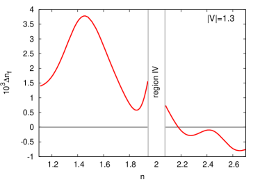
Figure 3: Difference between uncorrelated and correlated $f$-electron number, $\Delta n_{f}\equiv\sum_{\sigma}\langle\hat{n}_{{\bf i}\sigma}^{f}\rangle_{G}-\sum_{\sigma}\langle\hat{n}_{{\bf i}\sigma}^{f}\rangle_{0}$ along the line of constant hybridization, $|V|=1.3$, with respect to changing total filling. The specific character of the region IV is explained in Sec. IV.

IV.2 Correlated Fermi liquid

Before the detailed analysis is carried out, a methodological remark is in place. The effective Hamiltonian (13) is of single-particle form, but coupled to the self-consistent procedure of evaluating the relevant averages (22). However, this does not compose the full picture. The physical quantities are those obtained with a projected wave function. For example, $n_{f}\equiv\sum_{\sigma}\langle\psi_{G}|\hat{f}_{{\bf i}\sigma}^{\dagger}\hat{f}_{{\bf i}\sigma}|\psi_{G}\rangle=\sum_{\sigma}\langle\mathcal{P}_{G}\hat{n}_{{\bf i}\sigma}^{f}\mathcal{P}_{G}\rangle_{0}$, which in general is slightly different from $\sum_{\sigma}\langle\hat{n}_{{\bf i}\sigma}^{f}\rangle_{0}$. The situation is illustrated explicitly in Fig. 3. In effect, the quasiparticle picture is amended with the nonstandard features of this correlated (quantum) liquid (CL). Parenthetically, the same difference will appear when considering magnetic and superconducting states, where the magnetic moments, $\langle\hat{S}_{{\bf i}}^{z}\rangle_{G}$ vs. $\langle\hat{S}_{{\bf i}}^{z}\rangle_{0}$, and the superconducting gaps, $\langle\hat{\Delta}_{{\bf i}{\bf j}}\rangle_{G}$ and $\langle\hat{\Delta}_{{\bf i}{\bf j}}\rangle_{0}$ will be different. So, we have a mapping of the correlated onto quasiparticle states, but not of the physical properties. In brief, we have to distinguish between the correlated and the uncorrelated $f$-electron occupancy or other property even though, from the way of constructing (13), the density of quasiparticle states (coming from (13)), represents that in the correlated state.

IV.3 Quasiparticle Density of States

We start with analysis of the quasiparticle DOS emerging from the DE-GWF method in successive orders of the expansion (cf. Fig. 4). For $k>0$ and the total filling $n=1.97$ (i.e., near the half filling), the hybridization peaks become more pronounced (cf. Fig.4-the inset Table) and the hybridization gap increases.

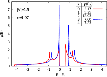
Figure 4: (Color online) Density of states (DOS) near the half-filling ($n=1.97$) at $|V|=1.5$ for selected orders of the diagrammatic expansion ($k=0,3$). Explicit values of $\rho(E_{F})$ are also listed in the inset Table (for $0\leq k\leq 4$). For $k=3$ a satisfactory convergence of the expansion is reached. The $k=1,2,4$ plots are not included for clarity as, apart from peak heights, they are practically the same as the plot for $k=3$. For $k>0$ (beyond GA) the hybridization peaks are more pronounced (large DOS at the Fermi level $\rho(E_{F})$), which is related directly to the increased by correlation effective-mass enhancement for quasiparticles.

For $k>0$ the overall shape of DOS changes only quantitatively (cf. Fig. 4). However, the value of the DOS at the Fermi level, $\rho(E_{F})$, changes remarkably (cf. the inset to Fig. 4). Although for $k=1$ it is underestimated and for $k=2$ overestimated, for $k=4$ we see no significant difference with respect to the $k=3$ case. For this reason, if not specified explicitly, the subsequent analysis is proceeded in the third order, $k=3$.

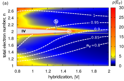
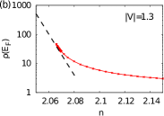
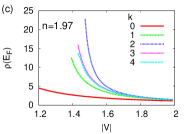
Figure 5: (Color online) (a) Density of states at the Fermi level $\rho(E_{F})$ on the hybridization strength – total electron concentration plane, $|V|$ – $n$. Additionally (not marked), for $n=2$ we obtain always the Kondo insulating state. By IV (for consistency with Fig.7) we have marked a V-shaped region where we have no numerical convergence due to the presence of singular hybridization peaks for low $|V|$ and with $n$ near the half filling (see main text). (b) Evolution of $\rho(E_{F})$ in the half-logarithmic scale near the region IV (along the vertical arrow with the letter b). By extrapolation (dashed line in (b)), for the almost half-filled situation, $\rho(E_{F})$ can be enhanced even by factor of 1000 relative to its lowest values on the $|V|$ – $n$ plane. (c) Evolution of $\rho(E_{F})$ with the decreasing $|V|$ (along the horizontal arrow with letter c), within successive orders of the expansion ($k\leq 4$). For large $|V|\gtrsim 1.8$, GA ($k=0$ order) provides already realistic values of $\rho(E_{F})$.

The value of $\rho(E_{F})$ is of crucial importance. This parameter is a measure of the quasiparticle effective mass, as the latter is inversely proportional to the second derivative of the energy, $\nabla^{2}_{{\bf k}}E_{{\bf k}}$, at the Fermi surface, and thus is determined by $\rho(E_{F})$.

In Fig. 5a we draw the value of $\rho(E_{F})$ on the plane hybridization – total electron number (per site), $V$ – $n$. This quantity is particularly strongly enhanced near the half filling ($n\simeq 2$). In comparison to the lowest value $\rho(E_{F})\approx 0.75$, the maximal enhancement is of the order of 40. In Fig. 5b we present evolution of $\rho(E_{F})$ on the logarithmic scale with the decreasing total filling and approaching $n=2$ (vertical arrow in Fig. 5a marked by the encircled letter b ). The extrapolated value of $\rho(E_{F})$ may reach extremely high values of 1000 and even more (dashed line in Fig. 5b) in the region IV. Such feature could explain extremely high mass renormalization in some of HFS for large but finite value of the Coulomb interaction $U$.

The region where $\rho(E_{F})$ is enhanced strongly, is that with low hybridization $|V|$ values and for the total filling $n\simeq 1$. This region is strictly correlated with the position of the second pronounced peak in DOS (cf. Fig. 4) which therefore has its meaning as the Van Hove singularity. Additionally, for $n_{f}\simeq 1$, where the effects of correlations are the strongest, we observe also a large value of $\rho(E_{F})$. In that limit the stability of magnetic phases should be studied separately Howczak and Spałek (2012); Howczak et al. (2013).

As marked in Fig. 5a, near the total half-filling, $n\simeq 2$, we could not obtain a satisfactory convergence of our self-consistent procedure. This is attributed to the position of the chemical potential extremely close to the hybridization-induced peaks (significant when $n_{f}\gtrsim 0.9$). Technically, this leads to extreme fluctuations (out of our numerical precision) of the filling, effective hopping parameters, and the lines coming from the effective Hamiltonian (13), as they are sensitive to a slight change of the chemical potential position. For $n=2$ and nonzero hybridization, we obtain always the Kondo insulating state. However, strictly speaking, the true Kondo-type compensated state is demonstrated explicitly only if magnetic structure is taken into account explicitly Doradziński and Spałek (1997, 1998); Howczak and Spałek (2012).

In Fig. 5c we depict the $\rho(E_{F})$ evolution with the decreasing hybridization amplitude $|V|$ for $k\leq 4$. Our results show that for large $|V|$, GA ($k=0$) already is reasonable approximation. The situation changes as we approach the low-$|V|$ regime near the half-filling, where inclusion of higher-order contributions leads to a strong enhancement of $\rho(E_{F})$, as discussed above.

In summary, the quasiparticle mass is enhanced spectacularly near $n=2$ and in the regime of small hybridization $|V|$. The $f$-state occupancy is then $n_{f}\gtrsim 0.9$. This is the regime associated with the heavy-fermion and the Kondo-insulating states. We discuss those states in detail in what follows.

IV.4 $f$-electron direct itineracy

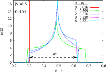
Figure 6: (Color online) $f$-electron density of states $\rho_{f}(E)$ within successive orders of expansion ($k\leq 4$). For $k=1$ and higher, formation of the effective $f$-band can be clearly observed. For $k=3$ the final shape of $\rho_{f}(E)$ and the value of $f$-band width $w_{f}$ stabilize.

As stated already, the DE-GWF method is used here to map the correlated (many-body) system, described by the original Hamiltonian (1) with the help of the Gutzwiller wave function $|\psi_{G}\rangle$, onto that described by the effective quasiparticle Hamiltonian (13) with an uncorrelated wave function $|\psi_{0}\rangle$. By constructing the effective Hamiltonian it is possible to extract the explicit contribution to the quasiparticle picture as coming from a direct hopping between the neighboring $f$ sites. By contrast, in GA ($k=0$) case, the $f$ electrons itineracy is only due to the admixture of $c$-states when the quasiparticle states are formed. Once we proceed with the diagrammatic expansion to higher order ($k>0$), they start contributing to the quasiparticle spectrum in the form of a dispersive $f$-band (cf. Fig. 6). The resulting band is narrow, $w_{f}\leq 0.5$, whereas the starting conduction ($c$) band has the width of $w_{c}=8$. As was mentioned in the Sec. I, we interpret the parameter $w_{f}$ as a measure of emerging degree of direct itineracy, i.e., presence of a direct hoppings between the neighboring $f$ states in the effective Hamiltonian.

Again, a methodological remark is in place here on the numerical convergence of the results with respect to $k$. Namely, the $f$-bandwidth appears already for $k=1$, but both its width and the curvature stabilizes only starting from $k=3$.

In the recent phenomenological modeling of CeCoIn₅ Aynajian et al. (2012); Allan et al. (2013); Dyke et al. (2014) the band structure used is the hybridized-two-band independent-particle model with dispersive $f$-band, even though the Ce 4$f$ states can be placed well above the so-called Hill limit, where there should not be any direct hopping between the original neighboring $f$ states. The fit presented there provides $w_{f}$ of the same order of magnitude as that obtained here. As those phenomenological models do not include the Coloumb interaction, the ground state is determined by the uncorrelated wave function. Hence, our analysis of the effective Hamiltonian resulting from ALM provides a direct microscopic rationalization of the narrow dispersive $f$-band presence assumed ad-hoc in the fitting procedure in Ref. Aynajian et al., 2012; Allan et al., 2013; Dyke et al., 2014.

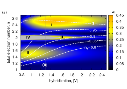
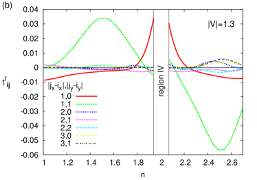
Figure 7: (Color online) (a) Effective bandwidth of $f$-states, $w_{f}$, on the hybridization strength $|V|$ – electron concentration $n$ plane. $w_{f}$ is regarded as a measure of direct itineracy of $f$-electron states. Three separate disjoint regions (light color) are regarded as universal and frequently discussed as separate limits, both in theory and experiment. Namely, the mixed valence regime (III), the Kondo/almost Kondo-insulating regime (II), and the Kondo-lattice regime (I) with $n_{f}\rightarrow 1-\delta$, $\delta\ll 1$. (b) Effective $f$-electron intersite hoppings $t^{f}_{{\bf i}{\bf j}}$ along the marked vertical line of the diagram for $|V|=1.3$. The energy dispersion for $f$ quasiparticles is determined mainly by the nearest and the second nearest hoppings $t^{f}_{{\bf i}{\bf j}}$. Region IV, near $n=2$ is marked separately due to the lack of convergence of the numerical results (see main text).

In Fig. 7a we display diagram comprising the width of $f$-band $w_{f}$ on $|V|$ – $n$ plane, with contours of constant values of $n_{f}$. We observe the appearance of regions, where the $f$ quasiparticles have a sizable bandwidth (bright color) and other, where they remain localized (dark regimes). We expect that in the regions, where $f$ electrons are forming a band, a nontrivial unconventional superconductivity and/or magnetism may appear. These topics should be treated separately as they require a substantial extension of the present approach (incorporating new type of lines) Kaczmarczyk et al. (2013, 2014); Kaczmarczyk (2015); Kaczmarczyk et al. (2015).

With the help of the width $w_{f}$ we may single out three physically distinct regimes (cf. Fig. 7a). We identify those regions as the mixed-valence regime (III), the Kondo/almost Kondo insulating regime (II), and the Kondo-lattice regime (I) with $n_{f}\rightarrow 1-\delta$, with $\delta\ll 1$ (cf. Fig. 7a). These universal regions are usually discussed independently within different specific models and methods. In regime I the role of $f$-$c$ Coulomb interactions (the Falicov-Kimball term) may be needed for completeness (cf. Ref. Miyake and Onishi, 2000), whereas in the Kondo-lattice regime the transformation to the Anderson-Kondo model is appropriate (cf. Refs. Howczak and Spałek, 2012; Howczak et al., 2013). In the extreme situation, the heavy-fermion states are modeled by pure Kondo-lattice modelSpałek (2015); Doniach (1987); Coqblin et al. (2003). However, strictly speaking, the last model applies only in the limit of localized $f$ electrons ($n_{f}=1$), since then the total numbers of $f$ and $c$ electrons are conserved separately.

In Fig. 7b we present the effective hopping parameters for $f$ states for $|V|=1.3$, i.e., along the marked vertical line in Fig. 7a. This line crosses three singled out regions of the itineracy. The leading contribution to the $f$-electron band energy arises from the nearest- and the second nearest-neighbor hoppings. Such circumstance confirms that our earlier assumption about the real-space cutoff shown in Fig. 2 has been selected properly. Moreover, it points to the importance of including also the components beyond those of the starting Hamiltonian, only rarely taken into account within the VMC method Watanabe et al. (2009); Liu et al. (2005).

In Fig. 8 we show the contributions to the effective hybridization. The initial (bare) local hybridization acquires momentum dependence. Nevertheless, the local part is still dominant since the nonlocal terms are at least two orders of magnitude smaller.

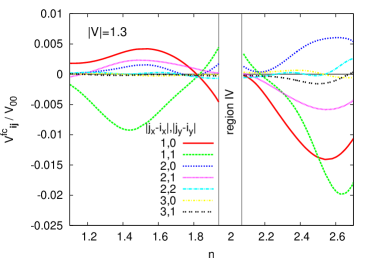
Figure 8: (Color online) Spatial contributions $V^{cf}_{{\bf i}{\bf j}}$ to the effective hybridization normalized by the first onsite (${\bf i}={\bf j}$) $V_{00}$ term along the marked vertical line of the diagram in Fig.7a for $|V|=1.3$. Note that due to correlation initially local, onsite hybridization acquires effectively momentum dependence. However, the nonlocal contributions constitute only up to 2% of the local one.

The emerging in our model $f$-band introduces a new definition of the $f$-electron itineracy as it is not so much connected to the Fermi-surface size Hoshino and Kuramoto (2013), but with the appearance of a direct hoppings between $f$ sites. This difference is highly nontrivial, especially in the limit $n_{f}=1$, where we obtain the largest bandwidth $w_{f}$. Such behavior is attributed to the specific character of our approach. Namely, we consider here the processes within our initial Hamiltonian (1), but under the assumption that the neighboring sites are also correlated. This, as we have shown directly, leads also to the finite $f$-band in the effective single particle Hamiltonian (13). The results thus throw a new light on the longstanding issue of the dual localized-itinerant nature of $f$ electrons in HFS Park et al. (2008); Troć et al. (2012). While the magnetism can be attributed to the almost localized nature of $f$ electrons, an unconventional superconductivity requires their itineracy in an explicit manner, as will be discussed elsewhere Wysokiński et al.

V Summary

We have applied a recently developed diagrammatic technique (DE-GWF) of evaluating the expectation values with the full Gutzwiller wave function for the case of two-dimensional Anderson lattice. We have analyzed properties of the model by discussing the most important features of the heavy fermion systems in the paramagnetic state. We have also shown that by approaching in successive orders of the expansion the full Gutzwiller-wave-function solution, we obtain a systematic convergence. In the zeroth order of expansion our method reduces to the standard Gutzwiller Approximation (GA).

In difference with GA, DE-GWF does not overestimate the hybridization narrowing factor. Furthermore, our method produces unusually enhanced peaks at the Fermi level in the density of states, particularly near the half-filling, $n\rightarrow 2$. This in turn, is connected to the value of effective mass and by analyzing in detail this region we can explain a very large mass enhancement observed in heavy fermion systems as described by ALM with large, but finite Coulomb-interaction value, here $U=10|t|$. The regions of sizable $\rho(E_{F})$ enhancement are also found in the small-hybridization limit and are connected to the presence of both the Van Hove singularity and the strong correlations in the limit of $n_{f}\rightarrow 1$.

The $f$-electron contribution to the full quasiparticle spectrum is analyzed in detail. For nonzero order of the expansion ($k>0$) we observe a systematic formation of the effective $f$-band with the increasing $k$. In spite of the fact that the bare electrons are initially localized, $f$ quasiparticles contribute to the total density of states as they become itinerant. We interpret this property as the emerging direct $f$-electron itineracy. As a measure of this behavior, we introduce the the width $w_{f}$ of effective $f$-band. Formation of such narrow $f$-band rationalizes e.g. the recent phenomenological modeling of the CeCoIn₅ band structure Aynajian et al. (2012); Allan et al. (2013); Dyke et al. (2014).

The nonstandard character of the resultant correlated Fermi liquid (CL) which differs from either the Landau Fermi liquid (FL) and the spin liquid (SL), should be stressed. FL represents a weakly correlated state (no localization) and SL represents a fully correlated state. Our CL state in this respect has an intermediate character. Namely, the quasiparticle states are formed (as exemplified by e.g. density of states), but the physical properties such as the occupancy $n_{f}$, the magnetic moment $\langle\hat{S}^{z}_{{\bf i}}\rangle$ or the pairing gap in real space $\langle\hat{\Delta}_{{\bf i}{\bf j}}\rangle$ are strongly renormalized by the correlations. Such situation is often termed as that of an almost localized Fermi-liquid state Fulde et al. (1988); Doradziński and Spałek (1997, 1998); Hewson (1993); Auerbach and Levin (1987).

By analyzing the results on the hybridization strength $|V|$ – total band filling $n$ plane, we single out explicitly three physically distinct regions, which we regard as three separate universality limits. Namely, we have linked those disjoint regions with the regimes frequently discussed as separate classes in the heavy fermion systems: the mixed-valence regime, the Kondo/almost Kondo insulating regime, and the Kondo-lattice regime for $n_{f}\rightarrow 1$. We suggest, that the regions of significant $f$-electron itineracy can be connected to the unconventional heavy fermion superconductivity which would require separate studies.

We have also commented on the longstanding issue of a dual localized-itinerant nature of $f$ electrons in the heavy fermion systems. The new definition of itineracy is in accord with their (almost) localized nature.

Appendix A Equivalence of the k=0 order DE-GWF expansion and the Gutzwiller approximation (GA)

Here we show the equivalence of the zeroth order DE-GWF and the standard Gutzwiller approximation (GA). In both methods (DE-GWF in the zeroth order of expansion $k=0$) the effect of the projection can be summarized by the expressions for evaluating following expectation values: $\langle\hat{n}_{{\bf i}\uparrow}\hat{n}_{{\bf i}\downarrow}\rangle_{G}$ and $\langle\hat{f}^{\dagger}_{{\bf i}\sigma}\hat{c}_{{\bf i}\sigma}+\text{H.c.}\rangle_{G}$. The remaining averages in ALM are unchanged under the projection.

Explicitly, in the DE-GWF for $k=0$ the resulting averages are expressed as follows

$$\langle\hat{n}_{{\bf i}\uparrow}\hat{n}_{{\bf i}\downarrow}\rangle_{G}^{(k=0)} =\lambda_{d}^{2}n_{0f}^{2}$$ (24a)

$$\langle\hat{f}^{\dagger}_{{\bf i}\sigma}\hat{c}_{{\bf i}\sigma}+\text{H.c.}\rangle_{G}^{(k=0)} =\alpha\langle\hat{f}^{\dagger}_{{\bf i}\sigma}\hat{c}_{{\bf i}\sigma}+\text{H.c.}\rangle_{0},$$ (24b)

where parameter $\alpha$ (see also Appendix B: Eqs. (29) and (30)) is defined as

$$\alpha\equiv(1-n_{0f})\lambda_{0}\lambda_{s}+n_{0f}\lambda_{d}\lambda_{s}.$$ (25)

On the other hand, in GA the resulting averages are expressed asRice and Ueda (1985)

$$\langle\hat{n}_{{\bf i}\uparrow}\hat{n}_{{\bf i}\downarrow}\rangle_{G}^{(GA)} =\langle n^{f}_{{\bf i}\uparrow}\hat{n}^{f}_{{\bf i}\downarrow}\rangle_{0}\equiv d^{2},$$ (26a)

$$\langle\hat{f}^{\dagger}_{{\bf i}\sigma}\hat{c}_{{\bf i}\sigma}+\text{H.c.}\rangle_{G}^{(GA)} =\sqrt{q}\langle\hat{f}^{\dagger}_{{\bf i}\sigma}\hat{c}_{{\bf i}\sigma}+\text{H.c.}\rangle_{0},$$ (26b)

where the parameter $d^{2}$ is the double occupancy probability, and $q$ is the so-called Gutzwiller factor reducing the hybridization amplitude, which for the equal number of particles for each spin is defined as

$$\sqrt{q}=\frac{\sqrt{(n_{0f}-d^{2})(1-2n_{0f}+d^{2})}+\sqrt{(n_{0f}-d^{2})d^{2}}}{\sqrt{n_{0f}(1-n_{0f})}}.$$ (27)

If we identify double occupancy probabilities expressed by both methods in (26a) and (24a) to be equal, yielding $d^{2}=\lambda_{d}^{2}n_{0f}^{2}$, then the parameter $\alpha$ (25) exactly reduces to the parameter $\sqrt{q}$ (27).

GA procedure results in the effective single-particle Hamiltonian of the form

$$\begin{gathered}\mathcal{\hat{H}}_{GA}\equiv\sum_{{\bf k},\sigma}\hat{\Psi}^{\dagger}_{{\bf k}\sigma}\begin{pmatrix}\epsilon_{{\bf k}}^{c}-\mu&\sqrt{q_{\sigma}}V\vspace{3pt}\\ \sqrt{q_{\sigma}}V&\epsilon_{f}-\mu\\ \end{pmatrix}\hat{\Psi}_{{\bf k}\sigma}+LUd^{2}\\ -\lambda^{f}_{n}\Big{(}\sum_{{\bf k},\sigma}\hat{n}^{f}_{{\bf k},\sigma}-Ln_{0f}\Big{)}-\lambda^{f}_{m}\Big{(}\sum_{{\bf k},\sigma}\sigma\hat{n}^{f}_{{\bf k},\sigma}-Lm_{f}\Big{)}.\end{gathered}$$ (28)

In the above Hamiltonian it is necessary to add constraints for $f$-electron concentration and their magnetization in order to satisfy consistency of the procedure Jȩdrak et al. ; Rice and Ueda (1986). In effect, the whole variational problem is reduced to minimization of the ground state energy with respect to $d^{2}$, $n_{0f}$, $m_{f}$, and respective Lagrange multipliers $\lambda_{n}^{f}$ and $\lambda_{m}^{f}$, playing the role of the effective molecular fields Jȩdrak et al. . However, the effect of constraint for $f$-electron magnetization is relevant only in the case of magnetism consideration either as intrinsicWysokiński et al. (2014, 2015) or induced by applied magnetic field Wysokiński and Spałek (2014). Here, as we discuss paramagnetic state $m^{f}=\lambda_{m}^{f}=\lambda_{n}^{f}=0$.

The DE-GWF method by construction guarantees that the variationally obtained $f$-electron occupancy number $n_{f}$ coincides with that obtained self-consistentlyKaczmarczyk (2015). We have thus provided analytical argument for the equivalence of the DE-GWF method for $k=0$ and the standard GA procedure. Also, by an independent numerical crosscheck we have verified that all the observables calculated within both methods indeed coincide.

Appendix B Diagrammatic sums

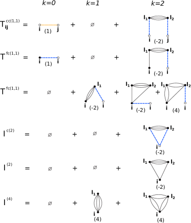
Figure 9: (Color online) Diagrammatic sums to the second order, $k=2$. $c$- and $f$- orbital sites are denoted with empty and filled circles respectively. Solid, dashed (blue) and dotted (orange) connections represent $F$, $W$, and $C$ lines respectively (cf. Eq. (10)). The numbers in brackets under diagrams stand for their multiplicity resulting from the Wick’s theorem. Note that by construction of our sums we have no diagrams with so-called “Hartree bubbles”, namely loop-lines within the same site and orbital.

We start with expressions for the following projected operators originating from ALM Hamiltonian (1), namely

$$\begin{split}\hat{P}_{G;{\bf i}}\hat{d}_{{\bf i}}\hat{P}_{G;{\bf i}}&=\lambda_{d}^{2}[2n_{0f}\hat{n}^{HF}_{{\bf i}}+(1-xd_{0})\hat{d}_{{\bf i}}^{HF}+d_{0}\hat{P}_{G;{\bf i}}^{2}],\vspace{2pt}\\ \hat{P}_{G;{\bf i}}\hat{n}_{{\bf i}\sigma}\hat{P}_{G;{\bf i}}&=(1+xm)\hat{n}^{HF}_{{\bf i}}+\gamma\hat{d}_{{\bf i}}^{HF}+n_{0f}\hat{P}_{G;{\bf i}}^{2},\vspace{2pt}\\ \hat{P}_{G;{\bf i}}\hat{f}_{{\bf i}\sigma}^{(\dagger)}\hat{P}_{G;{\bf i}}&=\alpha\hat{f}_{{\bf i}\sigma}^{(\dagger)}+\beta\hat{f}_{{\bf i}\sigma}^{(\dagger)}\hat{n}^{HF}_{{\bf i}},\end{split}$$ (29)

where additionally we have defined

$$\begin{split}\hat{n}^{HF}_{{\bf i}}&\equiv\hat{n}^{HF}_{{\bf i}\sigma}=\hat{n}^{HF}_{{\bf i}\bar{\sigma}},\\ \beta&\equiv\lambda_{s}(\lambda_{d}-\lambda_{0}),\\ \alpha&\equiv\lambda_{s}\lambda_{0}+\beta n_{0f},\\ \gamma&\equiv x(1-2n_{0f}),\\ d_{0}&\equiv n_{0f}^{2},\\ m&\equiv n_{0f}(1-n_{0f}).\end{split}$$ (30)

As mentioned in the main text, such form of the projected operators significantly speeds up the convergence of the numerical results Bünemann et al. (2012), since by construction all two-operator averages for a single site and $f$-orbital, the so-called Hartree bubbles, vanish. The above operator algebra leads to the compact definition of the diagrammatic sums: ${S\in\{T^{cc(1,1)}_{{\bf ij}},T^{fc(1,1)}_{{\bf ij}},T^{fc(3,1)}_{{\bf ij}},I^{c(2)},I^{(2)},I^{(4)}\}}$ in Eq. (11),

$$S=\sum_{k=0}^{\infty}\frac{x^{k}}{k!}S(k).$$ (31)

with the $k$-th order contributions

$$\begin{split}T^{cc(1,1)}_{{\bf ij}}(k)&\equiv\sum_{{\bf l}_{1},...,{\bf l}_{k}}\langle\hat{c}^{\dagger}_{{\bf i}\sigma}\hat{c}_{{\bf j}\sigma}\hat{d}^{HF}_{{\bf l}_{1},...,{\bf l}_{k}}\rangle_{0}^{c},\\ T^{fc(1[3],1)}(k)&\equiv\sum_{{\bf l}_{1},...,{\bf l}_{k}}\langle[\hat{n}^{HF}_{{\bf i}}]\hat{f}^{\dagger}_{{\bf i}\sigma}\hat{c}_{{\bf i}\sigma}\hat{d}^{HF}_{{\bf l}_{1},...,{\bf l}_{k}}\rangle_{0}^{c},\\ I^{c(2)}(k)&\equiv\sum_{{\bf l}_{1},...,{\bf l}_{k}}\langle\hat{n}^{c}_{{\bf i}\sigma}\hat{d}^{HF}_{{\bf l}_{1},...,{\bf l}_{k}}\rangle_{0}^{c},\\ I^{(2)}(k)&\equiv\sum_{{\bf l}_{1},...,{\bf l}_{k}}\langle\hat{n}^{HF}_{{\bf i}}\hat{d}^{HF}_{{\bf l}_{1},...,{\bf l}_{k}}\rangle_{0}^{c},\\ I^{(4)}(k)&\equiv\sum_{{\bf l}_{1},...,{\bf l}_{k}}\langle\hat{d}^{HF}_{{\bf i}}\hat{d}^{HF}_{{\bf l}_{1},...,{\bf l}_{k}}\rangle_{0}^{c}.\end{split}$$ (32)

Superscript $c$ in the expectation values means that only the connected diagrams are to be included. Note that in (32) there are no summation restrictions, due to the linked cluster theorem Fetter and Walecka (2003). The resulting diagrammatic sums for $S$ up to second order ($k=2$) are depicted in Fig. 9.

References

- Andres et al. (1975) K. Andres, J. E. Graebner, and H. R. Ott, Phys. Rev. Lett. 35, 1779 (1975).
- Stewart (1984) G. R. Stewart, Rev. Mod. Phys. 56, 755 (1984).
- Grewe and Steglich (1991) N. Grewe and F. Steglich, in Handbook on the Physics and Chemistry of Rare Earths, vol. 14 (Northe-Holland, Amsterdam, 1991).
- Fulde et al. (1988) P. Fulde, J. Keller, and G. Zwicknagl, in Solid State Physics, vol. 41 (Academic Press, New York, 1988).
- Ott (1987) H. R. Ott, in Progress in Low Temperature Physics, vol. XI (North-Holland, Amsterdam, 1987).
- Citro et al. (1999) R. Citro, A. Romano, and J. Spałek, Physica B 259-261, 213 (1999).
- Sheikin et al. (2003) I. Sheikin, A. Gröger, S. Raymond, D. Jaccard, D. Aoki, H. Harima, and J. Flouquet, Phys. Rev. B 67, 094420 (2003).
- McCollam et al. (2005) A. McCollam, S. R. Julian, P. M. C. Rourke, D. Aoki, and J. Flouquet, Phys. Rev. Lett. 94, 186401 (2005).
- Doradziński and Spałek (1997) R. Doradziński and J. Spałek, Phys. Rev. B 56, R14239 (1997).
- Doradziński and Spałek (1998) R. Doradziński and J. Spałek, Phys. Rev. B 58, 3293 (1998).
- Pfleiderer (2009) C. Pfleiderer, Rev. Mod. Phys. 81, 1551 (2009).
- Stewart (2001) G. R. Stewart, Rev. Mod. Phys. 73, 797 (2001).
- Löhneysen et al. (2007) H. v. Löhneysen, A. Rosch, M. Vojta, and P. Wölfle, Rev. Mod. Phys. 79, 1015 (2007).
- Lonzarich (2005) G. Lonzarich, Nature Physics 1, 5 (2005).
- Lacroix and Cyrot (1979) C. Lacroix and M. Cyrot, Phys. Rev. B 20, 1969 (1979).
- Hewson (1993) A. C. Hewson, The Kondo Problem to Heavy Fermions (Cambridge University Press, 1993).
- Auerbach and Levin (1987) A. Auerbach and K. Levin, J. Appl. Phys. 61, 3162 (1987).
- Howczak and Spałek (2012) O. Howczak and J. Spałek, J. Phys.: Condens. Matter 24, 205602 (2012).
- Howczak et al. (2013) O. Howczak, J. Kaczmarczyk, and J. Spałek, Phys. Status Solidi (b) 250, 609 (2013), ISSN 1521-3951.
- Gurin and Gulácsi (2001) P. Gurin and Z. Gulácsi, Phys. Rev. B 64, 045118 (2001).
- Gulácsi (2002) Z. Gulácsi, Phys. Rev. B 66, 165109 (2002).
- Gulácsi and Vollhardt (2003) Z. Gulácsi and D. Vollhardt, Phys. Rev. Lett. 91, 186401 (2003).
- Gulácsi and Vollhardt (2005) Z. Gulácsi and D. Vollhardt, Phys. Rev. B 72, 075130 (2005).
- Varma et al. (1986) C. M. Varma, W. Weber, and L. J. Randall, Phys. Rev. B 33, 1015 (1986).
- Gulácsi et al. (1993a) Z. Gulácsi, R. Strack, and D. Vollhardt, Phys. Rev. B 47, 8594 (1993a).
- Rice and Ueda (1985) T. M. Rice and K. Ueda, Phys. Rev. Lett. 55, 995 (1985).
- Rice and Ueda (1986) T. M. Rice and K. Ueda, Phys. Rev. B 34, 6420 (1986).
- Miyake et al. (1986) K. Miyake, S. Schmitt-Rink, and C. M. Varma, Phys. Rev. B 34, 6554 (1986).
- Fazekas (1999) P. Fazekas, Electron Correlation and Magnetism (World Scientific, Singapore, 1999).
- Kotliar and Ruckenstein (1986) G. Kotliar and A. E. Ruckenstein, Phys. Rev. Lett. 57, 1362 (1986).
- Spałek et al. (1987) J. Spałek, A. Datta, and J. M. Honig, Phys. Rev. Lett. 59, 728 (1987).
- Gebhard (1991) F. Gebhard, Phys. Rev. B 44, 992 (1991).
- Dorin and Schlottmann (1992) V. Dorin and P. Schlottmann, Phys. Rev. B 46, 10800 (1992).
- Dorin and Schlottmann (1993) V. Dorin and P. Schlottmann, Phys. Rev. B 47, 5095 (1993).
- Bünemann et al. (1998) J. Bünemann, W. Weber, and F. Gebhard, Phys. Rev. B 57, 6896 (1998).
- Jȩdrak and Spałek (2011) J. Jȩdrak and J. Spałek, Phys. Rev. B 83, 104512 (2011).
- Kaczmarczyk and Spałek (2011) J. Kaczmarczyk and J. Spałek, Phys. Rev. B 84, 125140 (2011).
- Abram et al. (2013) M. Abram, J. Kaczmarczyk, J. Jȩdrak, and J. Spałek, Phys. Rev. B 88, 094502 (2013).
- Ka̧dzielawa et al. (2013) A. P. Ka̧dzielawa, J. Spałek, J. Kurzyk, and W. Wójcik, Eur. Phys. J. B 86, 252 (2013).
- Zegrodnik et al. (2014) M. Zegrodnik, J. Bünemann, and J. Spałek, New J. Phys. 16, 033001 (2014).
- Wysokiński and Spałek (2014) M. M. Wysokiński and J. Spałek, J. Phys.: Condens. Matter 26, 055601 (2014).
- Wysokiński et al. (2014) M. M. Wysokiński, M. Abram, and J. Spałek, Phys. Rev. B 90, 081114(R) (2014).
- Wysokiński et al. (2015) M. M. Wysokiński, M. Abram, and J. Spałek, Phys. Rev. B 91, 081108(R) (2015).
- Edegger et al. (2006) B. Edegger, V. N. Muthukumar, and C. Gros, Phys. Rev. B 74, 165109 (2006).
- Lugas et al. (2006) M. Lugas, L. Spanu, F. Becca, and S. Sorella, Phys. Rev. B 74, 165122 (2006).
- Raczkowski et al. (2007) M. Raczkowski, M. Capello, D. Poilblanc, R. Frésard, and A. M. Oleś, Phys. Rev. B 76, 140505 (2007).
- Edegger et al. (2007) B. Edegger, V. N. Muthukumar, and C. Gros, Advances in Physics 56, 927 (2007).
- Chou et al. (2012) C.-P. Chou, F. Yang, and T.-K. Lee, Phys. Rev. B 85, 054510 (2012).
- Liu et al. (2005) J. Liu, J. Schmalian, and N. Trivedi, Phys. Rev. Lett. 94, 127003 (2005).
- Watanabe et al. (2009) T. Watanabe, H. Yokoyama, K. Shigeta, and M. Ogata, New J. Phys. 11, 075011 (2009).
- Asadzadeh et al. (2013) M. Z. Asadzadeh, F. Becca, and M. Fabrizio, Phys. Rev. B 87, 205144 (2013).
- Watanabe et al. (2015) H. Watanabe, K. Seki, and S. Yunoki, Phys. Rev. B 91, 205135 (2015).
- Jastrow (1955) R. Jastrow, Phys. Rev. 98, 1479 (1955).
- Bünemann et al. (2012) J. Bünemann, T. Schickling, and F. Gebhard, Eur. Phys. Lett. 98, 27006 (2012).
- Kaczmarczyk et al. (2013) J. Kaczmarczyk, J. Spałek, T. Schickling, and J. Bünemann, Phys. Rev. B 88, 115127 (2013).
- Kaczmarczyk et al. (2014) J. Kaczmarczyk, J. Bünemann, and J. Spałek, New J. Phys. 16, 073018 (2014).
- Kaczmarczyk (2015) J. Kaczmarczyk, Phil. Mag. 95, 563 (2015).
- Kaczmarczyk et al. (2015) J. Kaczmarczyk, T. Schickling, and J. Bünemann, Phys. Status Solidi B. (2015).
- Aynajian et al. (2012) P. Aynajian, E. H. da Silva Neto, A. Gyenis, R. E. Baumbach, J. D. Thompson, Z. Fisk, E. D. Bauer, and A. Yazdani, Nature 486, 201 (2012).
- Allan et al. (2013) M. P. Allan, F. Massee, D. K. Morr, J. S. Dyke, A. W. Rost, A. P. Mackenzie, C. Petrovic, and J. C. S. Davis, Nature Physics 9, 468 (2013).
- Dyke et al. (2014) J. S. Dyke, F. Massee, M. P. Allan, J. C. S. Davis, C. Petrovic, and D. K. Morr, Proc. Natl. Acad. Sci. 111, 11663 (2014).
- Holmes et al. (2004) A. T. Holmes, D. Jaccard, and K. Miyake, Phys. Rev. B 69, 024508 (2004).
- Ślebarski and Spałek (2005) A. Ślebarski and J. Spałek, Phys. Rev. Lett. 95, 046402 (2005).
- Ślebarski et al. (2010) A. Ślebarski, J. Spałek, M. Fijałkowski, J. Goraus, T. Cichorek, and L. Bochenek, Phys. Rev. B 82, 235106 (2010).
- Szlawska et al. (2009) M. Szlawska, D. Kaczorowski, A. Ślebarski, L. Gulay, and J. Stȩpień-Damm, Phys. Rev. B 79, 134435 (2009).
- Kaczorowski and Ślebarski (2010) D. Kaczorowski and A. Ślebarski, Phys. Rev. B 81, 214411 (2010).
- Watanabe and Miyake (2010) S. Watanabe and K. Miyake, Phys. Rev. Lett. 105, 186403 (2010).
- Tsunetsugu et al. (1997) H. Tsunetsugu, M. Sigrist, and K. Ueda, Rev. Mod. Phys. 69, 809 (1997).
- (69) In principle, the hybridization can have an intersite character Ghaemi et al. (2008).
- Gebhard (1990) F. Gebhard, Phys. Rev. B 41, 9452 (1990).
- Gulácsi et al. (1993b) Z. Gulácsi, M. Gulácsi, and B. Jankó, Phys. Rev. B 47, 4168 (1993b).
- Fetter and Walecka (2003) A. L. Fetter and J. D. Walecka, Quantum Theory of Many-Particle Systems (Dover Publications, New York, 2003).
- (73) M. Galassi, J. Davies, J. Theiler, B. Gough, G. Jungman, P. Alken, M. Booth, and F. Rossi, GNU Scientific Library Reference Manual (3rd Ed.), ISBN 0954612078.
- Miyake and Onishi (2000) K. Miyake and Y. Onishi, J. Phys. Soc. Jpn. 69, 355 (2000).
- Spałek (2015) J. Spałek, Phil. Mag. 95, 661 (2015).
- Doniach (1987) S. Doniach, Phys. Rev. B 35, 1814 (1987).
- Coqblin et al. (2003) B. Coqblin, C. Lacroix, M. A. Gusmão, and J. R. Iglesias, Phys. Rev. B 67, 064417 (2003).
- Hoshino and Kuramoto (2013) S. Hoshino and Y. Kuramoto, Phys. Rev. Lett. 111, 026401 (2013).
- Park et al. (2008) T. Park, M. J. Graf, L. Boulaevskii, J. L. Sarrao, and J. D. Thompson, Proc. Natl. Acad. Sci. 105, 6825 (2008).
- Troć et al. (2012) R. Troć, Z. Gajek, and A. Pikul, Phys. Rev. B 86, 224403 (2012).
- (81) M. M. Wysokiński, J. Kaczmarczyk, and J. Spałek, unpublished.
- (82) J. Jȩdrak, J. Kaczmarczyk, and J. Spałek, arXiv:1008.0021.
- Ghaemi et al. (2008) P. Ghaemi, T. Senthil, and P. Coleman, Phys. Rev. B 77, 245108 (2008).