Vector magnetometry based on $\mathrm{S=3/2}$ electronic spins

Abstract

Electronic spin systems with $\mathrm{S>1/2}$ provide an efficient method for DC vector magnetometry, since the conventional electron spin resonance spectra at a given magnetic field reflect not only the field strength but also orientation in the presence of strong spin-spin interactions. S=1 spins, e.g. the nitrogen-vacancy centers in diamond, have been intensively investigated for such a purpose. In this report, we compare S=1 and S=3/2 spins, and discuss how one can apply general principles for the use of high spin systems as a vector magnetometer to the S=3/2 spin systems. We find analytical solutions which allow a reconstruction of the magnetic field strength and polar angle using the observed resonance transitions if an uniaxial symmetry exists for the spin-spin interaction as in S=1 systems. We also find that an ambiguity of determining the field parameters may arise due to the unique properties of S=3/2 systems, and present solutions for it utilizing additional transitions in the low-field region. The electronic spins of the silicon vacancy in silicon carbide will be introduced as a model for the S=3/2 DC vector magnetometer and the practical usage of it, including the magic-angle spinning type method, will be presented too.

I Introduction

Electronic spins in highly localized defects, such as the nitrogen-vacancy (NV) centers in diamond Doherty et al. (2013); Schirhagl et al. (2014) and vacancy related defects in silicon carbide (SiC) Sörman et al. (2000); Janzén et al. (2009); Widmann et al. (2015); Christle et al. (2015); Weber et al. (2010); Koehl et al. (2011); Baranov et al. (2011); Mizuochi et al. (2002); Kraus et al. (2014a); Szász et al. (2015); Gali et al. (2010); Son et al. (2006), may experience a strong spin-spin interaction, e.g., a dipole-dipole interaction, which results in the so-called zero-field splitting (ZFS), partially (or completely) lifting degeneracy of energy eigenstates at zero magnetic field Stevenson (1984); Atherton (1993). If this interaction is strong enough, the eigenvalues of the spin Hamiltonian show a strong dependence on the orientation of the applied magnetic field. Such dependence causes a non linear shift of resonance transitions in electron spin resonance (ESR) spectra. Thus, the information about the applied external magnetic field can be extracted from ESR spectra provided the ZFS is known.

One well-known example is the NV center in diamond. Its application to DC field vector magnetometry has been reported and well understood in the field strength from sub-$\mathrm{\mu T}$ to a few tenth T Balasubramanian et al. (2008); Steinert (2010); Clevenson et al. (2015); Taylor et al. (2008). The NV center has a triplet ground state of $\mathrm{S=1}$ and when shifts of the ESR transition at a given DC magnetic field are directly monitored in the frequency domain, typically a $\mathrm{\sim 0.1~{}mT}$ minimum detectable magnetic field is achieved Degen (2008). This resolution is limited by the ESR linewidth which can be broadened by strong RF fields thus lowering the resolution. Lower RF power can be used to avoid power broadening, but the decreased signal strength requires a very long accumulation time. If time-domain experiments, e.g. a Ramsey fringe experiment, in which the magnetic field strength is imprinted in the phase of the superpositioned state, is conducted, a large signal strength can be maintained without power broadening, thus a sensitivity up to $\sim\mathrm{0.4~{}\mu T/\sqrt{Hz}}$, limited by the $\mathrm{T_{2}^{*}}$ of $\mathrm{\sim 1~{}\mu s}$, can be realized using a single NV center Taylor et al. (2008); Schirhagl et al. (2014). Further enhancement (below $\mathrm{1~{}nT/\sqrt{Hz}}$) is possible by using the NV center ensemble combined with the lock-in detection Clevenson et al. (2015). When the NV center is used for AC magnetic field sensing, spin echo type measurements can be used in which the long coherence time allows high sensitivity up to $\mathrm{\sim 1~{}nT/\sqrt{Hz}}$ using a single NV Balasubramanian et al. (2009) and $\mathrm{\sim 0.9~{}pT/\sqrt{Hz}}$ using an NV ensemble Wolf et al. (2014).

Higher spin systems ($\mathrm{S>1}$) can also be used as a vector magnetometer in a similar way. For example, the silicon vacancy ($\mathrm{V_{Si}}$) in silicon carbide (SiC) is known to possess a quartet manifold of $\mathrm{S=3/2}$ in its electronic ground state Mizuochi et al. (2003); Isoya et al. (2008); Mizuochi et al. (2005). Because its ESR signal can be detected at ambient condition Janzén et al. (2009); Soltamov et al. (2012); Simin et al. (2015); Kraus et al. (2014b); Janzén et al. (2009); Kraus et al. (2014a) even from a single defect Widmann et al. (2015) and the ZFS is in a range around a few mT depending on the polytype of SiC Janzén et al. (2009); Sörman et al. (2000), its application as a DC magnetometer has been suggested Kraus et al. (2014b); Simin et al. (2015). Note that Simin et al., have recently shown an experimental application of $\mathrm{V_{Si}}$ in SiC as a sub-mT DC magnetometer based on approximated solutions for the spin Hamiltonian at weak magnetic fields Simin et al. (2015).

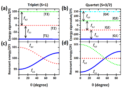
Figure 1: (Color online) Energy eigenvalues and ESR transition energies of high spin systems as a function of orientation at a high magnetic field $g\mu_{B}$$\mathrm{B_{0}}=100\times\mathrm{ZFS}$. (a) and (b) are the eigenvalues of the spin triplet (S=1) and quartet (S=3/2) state calculated numerically from Eq.(1), respectively. For numerical calculation, $D,E>0$, and an uniaxial symmetry $E\ll D$ are assumed thus only the polar angle, $\theta$ dependence is shown. Eigenstates are labeled in ascending order of corresponding energy eigenvalues. The most dominant transitions are indicated by the solid arrows with labels $f_{i,j}$ indicating a transition between $\mathrm{|i\rangle}$ and $\mathrm{|j\rangle}$. They are shown in (c) and (d) for the spin triplet and quartet states, respectively. All the energy values are normalized by ZFS.

In a spin system with a spin quantum number $\mathrm{S}$, the strength and orientation of the applied magnetic field vector $\mathbf{B_{0}}$ determines the Zeeman splitting, thus one should experimentally obtain the Zeeman splitting to get information about $\mathbf{B_{0}}$. For $\mathrm{S=1/2}$, the Zeeman splitting is calculated from an observed single resonant transition energy $h\nu=g\mu_{B}B_{0}$ where g is the Landé g-factor, $\mu_{B}$ is the Bohr magneton, and $h$ is Planck’s constant. The information for the orientation can be extracted only if $g$ is anisotropic. In high spin systems, the orientation related terms remain in the eigenvalue equation which result in the orientation dependent shift of ESR spectra, which cannot be explained by $g\mu_{B}B_{0}$. It is, therefore, mandatory to reconstruct the energy eigenstates using the observed resonant energies. Because there exist 2S+1 eigenstates, 2S resonant transition energies should be experimentally determined. For example, when the applied magnetic field strength is much larger than the ZFS, i.e., $g\mu_{B}$$|\mathbf{B_{0}}|\gg\mathrm{ZFS}$, at least two transition energies should be known for $\mathrm{S=1}$ while three values are necessary for $\mathrm{S=3/2}$ as explained in Fig.1. In this high field range, the two transitions for $\mathrm{S=1}$ and two out of the three transitions for $\mathrm{S=3/2}$ cross each other as shown in Figs.1(c) and 1(d). This leads to ambiguity in determining which observed ESR peak corresponds to which transition energy experimentally. In this report, we discuss how this ambiguity can be removed and thus show how to use the $\mathrm{S=3/2}$ system for vector magnetometry. For this, we will provide analytical solutions for the given $\mathrm{\mathbf{B_{0}}}$ vector as a function of the resonant transition energies. We will present $\mathrm{V_{Si}}$ spins in SiC as a model system and also a novel magnetometry scheme using the magic angle. The discussion in this report is also applicable to other $\mathrm{S=3/2}$ systems which have been found in fullerene Morton et al. (2005); Knapp et al. (1998); Harneit (2002); Benjamin et al. (2006); Mizuochi et al. (1999), organic molecules Teki et al. (2001); Kothe et al. (1980); Teki et al. (2008), Ni impurities in diamond Isoya et al. (1990), and calcium oxide crystals van Leeuwen et al. (1986).

II Vector magnetometry based on S=3/2 spins

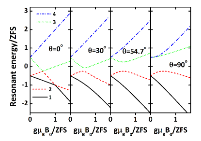
Figure 2: (Color online) $B_{0}$ dependence of the energy eigenvalues of a spin quartet state at various magnetic field orientations. Eigenstates are labeled in ascending order of the corresponding energy eigenvalues. As $B_{0}\rightarrow\infty$ at $\theta=0\,\degree$, $\mathrm{|4\rangle\rightarrow|m_{S}=+3/2\rangle}$, $\mathrm{|3\rangle\rightarrow|m_{S}=+1/2\rangle}$, $|\mathrm{2\rangle\rightarrow|m_{S}=-1/2\rangle}$, and $|\mathrm{1\rangle\rightarrow|m_{S}=-3/2\rangle}$.

In order to derive formulas for $B_{0}\equiv|\mathrm{\mathbf{B_{0}}}|$ and its orientation expressed by only three transition energies for $\mathrm{S=3/2}$, we will first construct the electronic spin Hamiltonian consisting of the ZFS and Zeeman term. The ZFS in high spin systems can be described by the dipole-dipole interaction term in the spin Hamiltonian, $\mathrm{\mathbf{S\cdot D\cdot S}}$ where $\mathrm{\mathbf{D}}$ is the dipole-dipole coupling tensor. For simplicity, we assume an isotropic Landé $g$-factor. Therefore in the principal axis system of $\mathrm{\mathbf{D}}$, in which the z-axis is set to the symmetry axis, the electronic spin Hamiltonian at $\mathrm{\mathbf{B_{0}}}$, is

$$H=g\mu_{B}\mathbf{B_{0}}\cdot\mathbf{S}+D\{S_{z}^{2}-S(S+1)/3\}+E(S_{+}^{2}+S_{-}^{2})/2,$$ (1)

where $E$ and $D$ are the ZFS parameters, assumed to be positive, and $E\ll D$ if an uniaxial symmetry exists. For S=3/2, the eigenvalue equation from Eq.(1) is, in the polar coordinate system,

$$\lambda^{4}-(2D^{2}+6E^{2}+\frac{5}{2}\beta_{0}^{2})\lambda^{2}-2\beta_{0}^{2}\{D(3\cos^{2}\theta-1)+3E\sin^{2}\theta\cos 2\phi\}\lambda$$

$$+\frac{9}{16}\beta_{0}^{4}+D^{4}-\frac{1}{2}D^{2}\beta_{0}^{2}-D^{2}\beta_{0}^{2}(3\cos^{2}\theta-1)+3E^{2}(3E^{2}+2D^{2})$$

$$+E\beta_{0}^{2}(6D\sin^{2}\theta\cos 2\phi+\frac{9}{2}E\cos 2\theta)=0,$$ (2)

where $\beta_{0}\equiv g\mu_{B}B_{0}$. The numerically calculated eigenvalues at various orientations are shown in Fig.2. When $\mathbf{B_{0}}$ is either parallel or perpendicular to the symmetry axis, the closed form solutions for each eigenvalue can be found as Atherton (1993)

$$\lambda = \frac{1}{2}\beta_{0}\pm\sqrt{(D+\beta_{0})^{2}+3E^{2}}\,\,\,\mathrm{or}\,\,\,-\frac{1}{2}\beta_{0}\pm\sqrt{(D-\beta_{0})^{2}+3E^{2}}\,\,\,\mathrm{for}\,\,\,\mathbf{B_{0}}\|\mathrm{z-axis},$$

$$\lambda = \frac{1}{2}\beta_{0}\pm\sqrt{\beta_{0}^{2}+D^{2}+3E^{2}-(D-3E)\beta_{0}}\,\,\,\mathrm{or}$$ (3)

$$-\frac{1}{2}\beta_{0}\pm\sqrt{\beta_{0}^{2}+D^{2}+3E^{2}+(D-3E)\beta_{0}}\,\,\,\mathrm{for}\,\,\,\mathbf{B_{0}}\parallel\mathrm{x-axis},$$

which gives the eigenvalues at zero magnetic field, $\lambda_{B_{0}=0}=\pm\mathrm{ZFS}/2$ where $\mathrm{ZFS}\equiv 2\sqrt{D^{2}+3E^{2}}$. The eigenvalue equation for the general case can be expressed as,

$$\sum_{n=0}^{2S+1}C_{n}\lambda^{n}=0.$$ (4)

By plugging each eigenvalue $\lambda_{i}$ into Eq.(4), one can obtain 2S+1 equations. The basic idea in order to find formulas for the $\mathrm{\mathbf{B_{0}}}$ vector expressed by the observed resonant energies, is to remove all $\lambda_{i}$ terms using the transition energy $f_{i,i-1}\equiv\lambda_{i}-\lambda_{i-1}$. Note that the energy eigenstates are not necessarily sorted with respect to the corresponding energy values. In other word, the indices can be randomly assigned to the states. Here, however, we keep the relation, $\lambda_{i}>\lambda_{i-1}$, for convenience. We follow this approach which has been frequently used for S=1 systems Balasubramanian et al. (2008); de Groot and van der Waals (1960). First, (2S-1) sets of three simultaneous equations are obtained by plugging $\lambda_{i}+f_{i+1,i}$, $\lambda_{i}$, and $\lambda_{i}-f_{i,i-1}$ (i=2,3,..2S) into Eq.(4). In each set, calculating

$$\sum_{n=0}^{2S+1}\frac{C_{n}\{(\lambda_{i}+f_{i+1,i})^{n}-\lambda_{i}^{n}\}}{C_{2S+1}}=0\,\,\mathrm{and}$$

$$\sum_{n=0}^{2S+1}\frac{C_{n}\{(\lambda_{i}-f_{i,i-1})^{n}-\lambda_{i}^{n}\}}{C_{2S+1}}=0,$$ (5)

results in two new simultaneous equations

$$\sum_{n=0}^{2S}C_{i,n}^{\prime}\lambda_{i}^{n}=0\,\,\mathrm{and}\,\,\sum_{n=0}^{2S}C_{i,n}^{\prime\prime}\lambda_{i}^{n}=0.$$ (6)

Again, by subtracting one from each other divided by the coefficient of the highest order term of each equation, respectively, as below

$$\sum_{n=0}^{2S}\frac{C_{i,n}^{\prime}\lambda_{i}^{n}}{C_{i,2S}^{\prime}}-\frac{C_{i,n}^{\prime\prime}\lambda_{i}^{n}}{C_{i,2S}^{\prime\prime}}=0,$$ (7)

we obtain a new equation for the eigenvalue of the energy eigenstate $|i\rangle$ in which the highest power is (2S-1),

$$\sum_{n=0}^{2S-1}C_{i,n}^{(2S-1)}\lambda_{i}^{n}=0,$$ (8)

where i=2,3,..2S. By repeating this procedure until only one linear equation for a single eigenvalue remains, one can find a formula for an eigenvalue expressed in terms of resonant energies, which allows us to find expressions for all other eigenvalues again using $f_{i,i-1}$. We use this procedure to find solutions for S=3/2.

Following the procedure explained above, we obtain two equations for two energy eigenvalues, $\lambda_{2}$ and $\lambda_{3}$, expressed by only $f_{2,1}$ and $f_{3,2}$, and $f_{3,2}$ and $f_{4,3}$, respectively, and $\mathrm{B_{0}}$, $\theta$, and $\phi$ which are present in both equations. Then using $f_{3,2}\equiv\lambda_{3}-\lambda_{2}$ once again, we obtain formulas for each eigenvalue expressed by only the resonant energies as below,

$$\lambda_{1} = -\frac{3}{4}f_{2,1}-\frac{1}{2}f_{3,2}-\frac{1}{4}f_{4,3},$$

$$\lambda_{2} = \frac{1}{4}f_{2,1}-\frac{1}{2}f_{3,2}-\frac{1}{4}f_{4,3},$$

$$\lambda_{3} = \frac{1}{4}f_{2,1}+\frac{1}{2}f_{3,2}-\frac{1}{4}f_{4,3},$$

$$\lambda_{4} = \frac{1}{4}f_{2,1}+\frac{1}{2}f_{3,2}+\frac{3}{4}f_{4,3}.$$ (9)

And by plugging one of these, e.g. $\lambda_{2}$, back into one of the equations found in the preceding steps, we finally obtain formulas for $\beta_{0}^{2}$, and a new quantity related to $\theta$ and $\phi$, $\eta\equiv E\mathrm{(2cos^{2}{\phi}\,sin^{2}{\theta}+cos^{2}{\theta})}+D\mathrm{\cos^{2}{\theta}}$,

$$\beta_{0}^{2} = \frac{(\frac{\sqrt{3}}{2}f_{4,3}+f_{3,2}+\frac{\sqrt{3}}{2}f_{2,1})^{2}+(1-\sqrt{3})(f_{4,3}+f_{2,1})f_{3,2}-f_{4,3}f_{2,1}-\mathrm{ZFS}^{2}}{5},$$ (10)

$$\eta = \frac{4[8(D+3E)+5(f_{4,3}-f_{2,1})]\beta_{0}^{2}+(f_{4,3}-f_{2,1})[4\mathrm{ZFS}^{2}-(f_{4,3}-f_{2,1})^{2}-4f_{3,2}^{2}]}{96\beta_{0}^{2}}.$$ (11)

Thus, in general, if $D$ and $E$ values are known and three resonant energies are observable, the applied magnetic field strength can be extracted from Eq.(10). In addition, if an uniaxial symmetry exists ($E\ll D$), because of $\eta\simeq D\cos^{2}{\theta}$, the polar angle can also be extracted from Eq.(11).

However, when one wants to use these formulas to find the external magnetic field vector, one may face a problem: how can one determine which observed resonant energy is from which transition? This is explained in Fig.1 and Fig.3. At a given magnetic field vector (e.g., $g\mu$$B_{0}\gg\mathrm{ZFS}$), there will appear three strong transitions for $\mathrm{S=3/2}$ as in Fig.3(a). The resonant energies are varying depending on the orientation for fixed $B_{0}$ and some of them even cross each other, thus it is hard to determine $f_{i,j}$ explicitly only taking into account these three transitions. However, in certain spin systems bound to certain localized defects in solids and at a certain magnetic field range, this ambiguity can be relaxed as will be shown in the following sections. We will focus on two distinguishable cases for $g\mu_{B}$$B_{0}\ll\mathrm{ZFS}$ and $g\mu_{B}$$B_{0}\gg\mathrm{ZFS}$. The case for $g\mu_{B}$$B_{0}\sim\mathrm{ZFS}$, however, will not be discussed because complex spectra appear due to a strong interaction among each eigenstate Degen (2008) via e.g. the level anti-crossing as in the NV centers He et al. (1993), thus, high spin systems are not an appropriate sensor for this field range. In the following sections, we will consider the uniaxial symmetry for all the numerical simulations unless noticed. This will allow us to utilize Eq.(11) to extract at least one orientation component, $\theta$.

II.1 High field, $g\mu_{B}$$B_{0}\gg\mathrm{ZFS}$

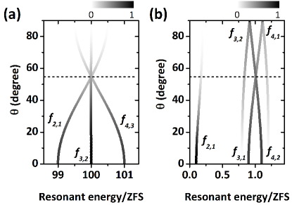
Figure 3: Orientation dependence of ESR transitions at (a) high ($g\mu_{B}B_{0}=100\times\mathrm{ZFS}$) and (b) low ($g\mu_{B}B_{0}=\mathrm{ZFS}/10$) magnetic field strength. The dashed lines indicate the magic angle $\theta_{m}$. The gray color scale depicts the normalized ESR transition probabilities for $\mathbf{B_{1}}\mathrm{\parallel x-axis}$

.

Figure 3(a) depicts how each transition evolves at varying orientation $\theta$ at high static magnetic fields ($g\mu_{B}$$B_{0}=100\times\mathrm{ZFS}$) together with ESR transition probabilities. $\mathbf{B_{1}}$ is assumed to have only an x-axis component. At high fields, three transitions are visible. Without knowing the information about $B_{0}$, it is not possible to assign them correctly because as will be seen later, there appears also three or even more than three resonances that originate from different transitions at low magnetic fields. However, one can guess $B_{0}$ roughly from the observed resonant energies because they are approximately proportional to $B_{0}$ at high field. For example, $f_{3,2}$ shows very weak orientation dependence thus can be used to estimate $B_{0}$. Once the $B_{0}$ scale is roughly guessed, one can try to assign the observed resonant energies. Because $f_{3,2}$ always stays in the middle of all resonance transitions, this can be explicitly determined. And because Eq.(10) is invariant under switching of $f_{4,3}$ and $f_{2,1}$, $B_{0}$ can be unambiguously extracted. In contrast, Eq.(11) will result in a systematic error if $f_{4,3}$ and $f_{2,1}$ are not correctly assigned. Thus, a magnetometer based on a $S=3/2$ system can be used only to extract $B_{0}$ at a high magnetic field. This is a disadvantage compared to $S=1$ because a similar equation to Eq.(11) is also invariant under switching of two observed resonant energies Balasubramanian et al. (2008). This problem, however, may be overcome by manipulating the ZFS Dolde et al. (2011). If the electric dipole moment is large enough and their contribution to the ZFS Hamiltonian, the Stark-effect, is well-known, manipulation of the ZFS by either applying an electric field Dolde et al. (2011) or pressure Falk et al. (2014) along a favored direction can result in the shifts of each ESR transitions in different manners. Thus monitoring the additional shift upon the change in ZFS, may allow to determine all the necessary transitions and subsequently Eq.(11) can be used without systematic errors.

II.2 Low field, $g\mu_{B}$$B_{0}\ll\mathrm{ZFS}$

Figure 3(b) shows that one can see up to five transitions at low field. At a small angle, there are three dominant transitions, $f_{2,1}$, $f_{3,1}$, and $f_{4,2}$, and two additional transitions, $f_{3,2}$, and $f_{4,1}$, which arise at large angle. Alternate forms of Eq.(10) and (11) using only the most dominant transitions can be found for small angles (not shown). These forms, however, are not useful because $f_{4,2}$ and $f_{3,1}$ are changing their relative positions at a larger angle. Instead, $f_{4,1}$ and $f_{3,2}$ can be used since their relative positions are not changing and in certain $S=3/2$ systems, e.g. $\mathrm{V_{Si}}$ in SiC (see section III), these transitions show good intensities at every orientation Simin et al. (2015). The other useful formulas can be found by plugging $f_{4,3}=f_{4,1}-f_{3,2}-f_{2,1}$ into Eqs.(10) and (11) as

$$\beta_{0}^{2} =\frac{(\sqrt{3}f_{avg}+f_{2,1})^{2}-2f_{4,1}f_{3,2}+(1-\sqrt{3})f_{3,2}f_{2,1}-(1+\sqrt{3})f_{41}f_{21}-\mathrm{ZFS}^{2}}{5},$$ (13)

$$\eta =\frac{1}{96\beta_{0}^{2}}\{4[8(D+3E)+5\Delta f_{out}-10f_{2,1}]\beta_{0}^{2}-8f_{2,1}(\mathrm{ZFS}^{2}-f_{2,1}^{2}-f_{3,2}^{2})$$

$$+\Delta f_{out}[4({\mathrm{ZFS}}^{2}-3f_{2,1}^{2}-f_{3,2}^{2})+\Delta f_{out}(6f_{2,1}-\Delta f_{out})]\},$$

where $\Delta f_{out}\equiv f_{4,1}-f_{3,2}$ and $f_{avg}\equiv(f_{3,1}+f_{4,2})/2=(f_{3,2}+f_{4,1})/2$. These are useful, because if $f_{4,1}$ and $f_{3,2}$ are observable together with $f_{4,2}$ and $f_{3,1}$, one always can unambiguously determine the two outermost transitions, and $f_{4,2}$ and $f_{3,1}$ are not in use or necessary only for calculating $f_{avg}$.

So far, the strategies to use $S=3/2$ systems as a DC vector magnetometer have been discussed in both high and low magnetic field ranges. Though only $B_{0}$ can be obtained at high fields using only a conventional experimental method, both $B_{0}$ and polar angle can be determined at low field. However, in many high spin systems bound to localized defects in solids, spin-dependent intersystem-crossing may induce a strong polarization into specific spin states as in $\mathrm{V_{Si}}$ in SiC Mizuochi et al. (2002); Isoya et al. (2008). Thus, some transitions may be hardly observable. In addition, because only the polar angle can be obtained, it is still not possible to realize a genuine vector magnetometry. In the following sections, we will present $S=3/2$ spins of $\mathrm{V_{Si}}$ in SiC as a model system and discuss the practical usage of them and a possible way to use them as a vector magnetometer.

III Silicon vacancy spins in silicon carbide as a DC vector magnetometer

We present $\mathrm{V_{Si}}$ in SiC as a model system to provide explanations about how the formulas, found in previous sections, can be used to experimentally reconstruct the applied external magnetic field vector. Because spin properties are different depending on the polytype, here we discuss only a specific polytype, namely 4H-SiC. In addition, because there exist two inequivalent lattice sites, there appear two different silicon vacancies with different ZFS, and we choose only one of them known as $T_{V2a}$ center Sörman et al. (2000); Janzén et al. (2009). In the $T_{V2a}$ center, it is known that there exist an uniaxial symmetry around the c-axis thus $E\ll D$ and $\mathrm{ZFS}/h\simeq 2D/h\simeq 70~{}\mathrm{MHz}$ Sörman et al. (2000); Janzén et al. (2009). It is also known that optical polarization results in equal populations in two substates, $|m_{S}=\pm 1/2\rangle$. This is responsible for the absence of a transition between $|m_{S}=+1/2\rangle$ and $|m_{S}=-1/2\rangle$ while aother two transitions, between $|m_{S}=+3/2\rangle$ and $|m_{S}=+1/2\rangle$, and between $|m_{S}=-3/2\rangle$ and $|m_{S}=-1/2\rangle$ are observable in the ESR spectra of $T_{V2a}$ for $\mathbf{B_{0}}||$c-axis Widmann et al. (2015); Soltamov et al. (2012); Sörman et al. (2000); Mizuochi et al. (2002); Kraus et al. (2014b, a); Simin et al. (2015); Baranov et al. (2011). In the $\mathbf{B_{0}}$ orientation dependence at low  Simin et al. (2015) and high magnetic fields Sörman et al. (2000); Mizuochi et al. (2002); Soltamov et al. (2012); Kraus et al. (2014b), one of the allowed transitions, corresponding to the transition between $|m_{S}=+1/2\rangle$ and $|m_{S}=-1/2\rangle$ for $\mathbf{B_{0}}||$c-axis, has not been observed probably due to that this equal population is somehow maintained. This will prevent Eq.(10), (11), (13), and (13) from being used because $f_{3,2}$ at high fields and $f_{2,1}$ at low fields will not be observable. This transition, however, can become visible once electron-electron double resonance (ELDOR) is applied. The population difference between $|m_{S}=\pm 1/2\rangle$ states can be induced by applying e.g. a resonant $\pi$ pulse between $|m_{S}=+3/2\rangle$ and $|m_{S}=+1/2\rangle$ (or $|m_{S}=-1/2\rangle$ and $|m_{S}=-3/2\rangle$) states which enable detection of this missing transition Isoya et al. (2008). This will allow unambiguous determination of one transition $f_{2,1}$ at low fields or $f_{3,2}$ at high fields experimentally.

At high magnetic field (e.g., $B_{0}\sim 300$$~{}mT$) as in Fig.3(a), two outer transitions, $f_{4,3}$ and $f_{2,1}$ have been observed experimentally at almost all orientations at both cryogenic  Mizuochi et al. (2002); Sörman et al. (2000) and room temperature Kraus et al. (2014b) except the central peak. The central peak is observable by ELDOR experiments Isoya et al. (2008), thus Eq.(10) can be used as explained in section (II.1). However, the polar angle, $\theta$, can be determined from Eq.(11) only at small angles because of the ambiguity on determining $f_{4,3}$ and $f_{2,1}$ at larger angles.

ESR spectra of $T_{V2a}$ centers at a low magnetic field (e.g. sub-mT) as in Fig.3(b) allow an unambiguous determination of both $B_{0}$ and polar angle as long as the ELDOR can be used to determine $f_{2,1}$ as explained in section (II.2). However, one can consider another case in which either ELDOR experiments are not available or $f_{2,1}$ is hardly observed in the ELDOR spectrum. In such a case, if $f_{4,1}$ and $f_{3,2}$ are observable, using relations $f_{3,1}+f_{4,2}=f_{3,2}+f_{4,1}$, $f_{4,3}=f_{4,2}-f_{3,2}$, and $f_{2,1}=f_{3,1}-f_{3,2}$ from Eq.(II), we again obtain alternative forms of Eqs.(10) and (11) as

$$B_{0}^{2}=\frac{(\sqrt{3}f_{avg}+f_{3,2})^{2}-f_{4,2}f_{3,1}-2(\sqrt{3}+1)f_{3,2}f_{avg}-\mathrm{ZFS}^{2}}{5},$$ (14)

$$\eta=\frac{[32(D+3E)+20\Delta f_{in}]B_{0}^{2}+\Delta f_{in}(4{\mathrm{ZFS}}^{2}-\Delta f_{i}^{2}-4f_{3,2}^{2})}{96B_{0}^{2}},$$ (15)

where $\Delta f_{in}\equiv f_{4,2}-f_{3,1}$. Note that $f_{3,2}$ appears in both formulas but because it is always the lowest energy transition, this can be explicitly determined. Similarly, one can find additional alternatives using $f_{4,1}$ instead of $f_{3,2}$. Therefore, even if ELDOR is not available, as long as either $f_{4,1}$ or $f_{3,2}$ is observable together with $f_{4,2}$ and $f_{3,1}$, $B_{0}$ can be extracted using Eq.(14) because it is invariant under switching $f_{4,2}$ and $f_{3,1}$. This scheme is feasible since $f_{4,1}$ and $f_{3,2}$ are observable from $\mathrm{T_{V2a}}$ in SiC by cw methods with a decent signal strength at sub-mT as recently reported Simin et al. (2015). Eq.(15), however, still cannot provide an unambiguous way to determine the polar angle because of $\Delta f_{in}$ which changes signs if $f_{4,2}$ and $f_{3,1}$ are not correctly determined.

So far, the strategies to use $\mathrm{V_{Si}}$ in SiC as a vector magnetometer has been discussed. While the magnetic field strength can be extracted in both high and low magnetic field range, the orientation can be extracted only if there exists an uniaxial symmetry at a low magnetic field, and the azimuthal angle cannot be determined in any case. Note that the S=1 system with the uniaxial symmetry also can provide only the polar angle. But in the case of the NV center in diamond, because the NV centers can be in four different orientations along the diamond bond axes, one can determine both the polar and azimuthal angles from the shift of transitions of the inequivalently oriented NV centers. Similarly, $\mathrm{V_{Si}}$ in inequivalent lattice sites, e.g. $\mathrm{T_{V1a}}$ and $\mathrm{T_{V2a}}$ in 4H-SiC, and $\mathrm{T_{V1a}}$, $\mathrm{T_{V2a}}$ and $\mathrm{T_{V3a}}$ in 6H-SiC Janzén et al. (2009) can also be utilized. However, ESR spectra of $\mathrm{T_{V1a}}$ and $\mathrm{T_{V3a}}$ are hardly visible at room temperature Janzén et al. (2009); Baranov et al. (2011); Soltamov et al. (2012). Thus, an alternate method relying only on the $\mathrm{T_{V2a}}$ center that can be used for any magnetic field strength at room temperature is necessary. In the next section, another method using a magic angle that allows for the use of S=3/2 as a vector magnetometer will be discussed.

IV Vector magnetometry using magic angle

We start from the eigenvalue equation in Eq.(II). In this equation, one can find terms including $\mathrm{(3cos^{2}{\theta}-1)}$, which becomes zero at the magic angle $\theta_{m}\simeq 54.7\,\degree$. Eq.(II) can be simplified for $\theta=\theta_{m}$ and $E\ll D$ as,

$$\lambda^{4}-(2D^{2}+\frac{5}{2}\beta_{0}^{2})\lambda^{2}+\frac{9}{16}\beta_{0}^{4}+D^{4}-\frac{1}{2}D^{2}\beta_{0}^{2}=0,$$ (16)

and the eigenvalues are simply

$$\lambda=\pm\frac{1}{2}\sqrt{4D^{2}+5\beta_{0}^{2}\pm 4\sqrt{3\beta_{0}^{2}D_{0}^{2}+\beta_{0}^{4}}},$$ (17)

as depicted in Fig.2(c). For high $B_{0}$, these can be again approximated as

$$\lambda=\pm\frac{3}{2}\beta_{0}\,\,\,\mathrm{or}\,\,\,\pm\frac{1}{2}\beta_{0}\,\,\,(\mathrm{for}\,\,\,g\mu_{B}B_{0}\gg\mathrm{ZFS}).$$ (18)

Thus, at $\theta_{m}$, we obtain $|\lambda_{1}|=|\lambda_{4}|$ and $|\lambda_{2}|=|\lambda_{3}|$, and can see the least number of transitions as seen in Fig.3. We can use this aspect to use $\mathrm{S=3/2}$ system as a vector magnetometer. If the spin sensor is being rotated around an axis and the orientation between the c-axis and the rotational axis is fixed to $\theta_{m}$, one expects to see the least number of transitions whose widths are the narrowest when the rotational axis is aligned to the applied external magnetic field. In contrast, when the rotational axis is misaligned, very broad ESR transitions appear due to orientation sweeping.

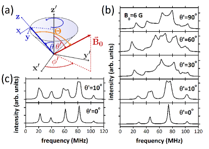
Figure 4: (Color online) Magic angle DC magnetometry based on a S=3/2 spin system. (a) describes the frames used for the numerical simulation. See text for details. (b) shows the numerical simulations of the cw ESR spectra when the S=3/2 spin is misaligned by $\theta=\theta_{m}$ relative to the rotational axis at various orientations of $\mathbf{B_{0}}$ vector in $\mathrm{y^{\prime}-z^{\prime}}$ plane at low field $B_{0}\mathrm{=6\,G}$. For the simulation, the ZFS of $T_{V2a}$ center in SiC, $\mathrm{ZFS}/h\simeq 2D/h\simeq 70\,\mathrm{MHz}$ is assumed. (c) shows the same simulation but for the case when $\theta\neq\theta_{m}$ and $\theta=30\,\degree$.

Figure 4 describes such an experiment in which the SiC crystal is attached to a rotational axis forming $\theta_{m}$ with respect to the c-axis of the crystal. The resonant RF can be applied using a miniature coil surrounding either the rotational axis or the SiC crystal, similar to what has been suggested for the quantum gyroscope based on the NV center Ajoy and Cappellaro (2012). For the detection, a small sized ESR cavity can be used for conventional ESR detection. Fiber coupling also can be considered for ODMR. If an electrically detected magnetic resonance is possible, which has recently been shown in high spin systems Bourgeois et al. (2015) and also in SiC Cochrane et al. (2012), additional small circuits can be utilized. $\mathrm{B_{1}}$ field modulation can be used to enhance the signal to noise ratio Lee et al. (2012) because the ELDOR experiment which requires $\mathrm{B_{1}}$ pulses is not necessary for this experiment. For the simulation of ESR spectra in this experiment, a laboratory frame is assumed: the $\mathrm{z^{\prime}-axis}$ is set to the rotational axis. The angle ($\Theta$) between the c-axis of the crystal, rotating with a constant speed around the $\mathrm{z^{\prime}-axis}$, and the external magnetic field can be derived and replace $\theta$ in Eq.(II). For convenience, the RF field is assumed to be in the x-axis of the rotating frame. By assuming a Lorentzian lineshape with 3 MHz FWHM, the numerically simulated ESR spectra at varying $\theta^{\prime}$ while $\phi^{\prime}$ is fixed to $90\,\degree$ are simulated for a low field ($B_{0}=6~{}G$) as shown in Fig.4(b). As expected, when $\theta^{\prime}=0$ equivalently $\Theta=\theta_{m}$ or $\bf{B_{0}}\parallel\mathrm{z^{\prime}-axis}$, the narrowest transitions are found while seriously broadened peaks like a powder pattern appears when misaligned ($\theta^{\prime}\neq 0$). Note that in order to present a general $\mathrm{S=3/2}$ case, $f_{2,1}$ is assumed to be visible in cw ESR spectra at low field. Therefore by monitoring the linewidth of the observed transition spectra while moving the rotational axis, $z^{\prime}$-axis, one can explicitly find the orientation of the external magnetic field. The field strength also can be extracted from the observed resonant energy of the strongest transition using Eq.(17). For very small field $g\mu_{B}$$B_{0}\ll\mathrm{ZFS}$, $f_{3,1}=f_{4,2}\approx$ $g\mu_{B}$$B_{0}+4$$g\mu_{B}$$B_{0}D^{2}/3$. We also can observe spectra consisting of the narrow transitions even if $\theta\neq\theta_{m}$ as long as $\theta^{\prime}=0$. However, because many transitions whose intensities are comparable to each other appear as in Fig.4(c), it is more convenient to use the magic angle because the most dominant transition is easily distinguishable.

V Conclusion

We have shown that using the $\mathrm{V_{Si}}$ in SiC as a model system, S=3/2 electronic spins with the uniaxial symmetry can be used to find the strength and polar angle of the applied external magnetic field if at least three ESR transitions can be found experimentally and the ZFS parameters are known. At a high $B_{0}$ field ($g\mu_{B}$$B_{0}\gg\mathrm{ZFS}$), $B_{0}$ can be obtained from the observed ESR spectra but the polar angle cannot be determined due to the ambiguity of differentiating two outer transitions. In contrast, at low $g\mu_{B}$$B_{0}$ ($\ll\mathrm{ZFS}$), as long as one can explicitly identify at least three transitions including the allowed lowest energy transition, the external magnetic field vector can be reconstructed. In the field strength comparable to the ZFS, it is hard to find a useful scheme because very complex patterns appear due to mixing of some of the eigenstates. In the case of the NV centers in diamond (ZFS/h=2.87 GHz), this missing range is around $\sim 100\,mT$. The $V_{Si}$ in SiC can fill out this gap since its ZFS is quite small ($\mathrm{ZFS}/h\sim 100\,\mathrm{MHz}$) thus this magnetic field range can be considered as a high field range in which the three necessary transitions are well observable Isoya et al. (2008); Kraus et al. (2014b), and at least the field strength can be experimentally determined. When the $V_{Si}$ in SiC is used to realize such schemes at sub-mT, if the lowest transition energy is observable by ELDOR, one can determine both $B_{0}$ and $\theta$ without ambiguity. Even if ELDOR is not available, thanks to the additional transitions that appear at low fields, the field strength can be determined.

The magic angle terms in the eigenvalue equation allow for an alternative method to use S=3/2 systems as a DC vector magnetometer. If the S=3/2 spins fixed in a crystal can be rotated around the rotational axis, the unambiguous determination of the applied magnetic field vector is feasible by monitoring the linewidth of the observed ESR spectra while the symmetry axis of the crystal is oriented at $\theta_{m}$ relative to the rotational axis and the rotational axis is moving. This configuration also can be realized by producing an array of the crystals such that the symmetry axes of each crystal form a cone whose opening angle is twice the magic angle.

These findings provide a better understanding of the S=3/2 electronic spin Hamiltonian, especially at low fields. They also provide an outlook for the application of $\mathrm{V_{Si}}$ in SiC to quantum magnetometry which is promising thanks to the electrical properties of SiC, which outstand the host material of the NV centers, and the mature fabrication technology, which allows an efficient fabrication of electronic devices even at the atomic scale Lohrmann et al. (2015).