Conformal type of ends of revolution in space forms of constant sectional curvature.

Abstract.

In this paper we consider the conformal type (parabolicity or non-parabolicity) of complete ends of revolution immersed in simply connected space forms of constant sectional curvature. We show that any complete end of revolution in the $3$-dimensional Euclidean space or in the $3$-dimensional sphere is parabolic. In the case of ends of revolution in the hyperbolic $3$-dimensional space, we find sufficient conditions to attain parabolicity for complete ends of revolution using their relative position to the complete flat surfaces of revolution.

1. Introduction.

Let $\Sigma$ be a complete and non-compact surface. Let $D\subset\Sigma$ be an open precompact subset of $\Sigma$ with smooth boundary. An end $E$ of $\Sigma$ with respect to $D$ is a connected unbounded component of $\Sigma\setminus D$. An end $E$ is parabolic ([MP04, Li00, Gri99]) if every bounded harmonic function on $E$ is determined by its boundary values.

This paper is concerned with the study of the conformal type (parabolicity or non-parabolicity) of complete ends of revolution immersed in the $3$-dimensional Euclidean space $\mathbb{R}^{3}$, in the $3$-dimensional hyperbolic space $\mathbb{H}^{3}$, or in the $3$-dimensional sphere $\mathbb{S}^{3}$. Let us denote by $\mathbb{M}^{3}(\kappa)$ the simply connected space form of constant sectional curvature $\kappa\in\mathbb{R}$. Hence, $\mathbb{M}^{3}(1)=\mathbb{S}^{3}$, $\mathbb{M}^{3}(0)=\mathbb{R}^{3}$, $\mathbb{M}^{3}(-1)=\mathbb{H}^{3}$. An end of a complete surface in $\mathbb{M}^{3}(\kappa)$ is a complete end of revolution if there exists a geodesic in $\mathbb{M}^{3}(\kappa)$ such that the end is invariant by the group of rotations of $\mathbb{M}^{3}(\kappa)$ that leaves this geodesic point-wise fixed. More precisely, an end of revolution will be the rotation along a geodesic ray $\gamma$ of $\mathbb{M}^{3}(\kappa)$ of a generating smooth curve $\beta:[0,\infty)\to\mathbb{M}^{2}(\kappa)$ contained in a totally geodesic hypersurface $\mathbb{M}^{2}(\kappa)$ where the ray $\gamma$ belongs. In order to guarantee the smoothness and that the end is the end of a complete surface we require that the generating curve $\beta$ be regular, with infinite longitude and does not intersect the geodesic ray $\gamma$.

The conformal type of a Riemannian manifold has been largely studied. In particular in [Tro99] sufficient and necessary conditions for the parabolicity of a manifold with a warped cylindrical end were provided, in [Gri99] rotationally symmetric manifolds were analyzed, and in the examples of [HP11, MP10] certain surfaces of revolution in $\mathbb{R}^{3}$ have been studied from an extrinsic approach. Our first result characterizes the conformal type of complete ends of revolution in $\mathbb{R}^{3}$ or in $\mathbb{S}^{3}$

Theorem A.

Any complete end of revolution in $\mathbb{R}^{3}$, or in $\mathbb{S}^{3}$, is a parabolic end.

The conformal classification of ends of revolution in $\mathbb{H}^{3}$ becomes more complicated. In the hyperbolic space there is no restriction on the conformal type of ends of revolution. Actually, in Section 9 we will show examples of parabolic and non-parabolic ends in $\mathbb{H}^{3}$. In the half space model of the hyperbolic space,

(1.1) $$\mathbb{H}^{3}:=\left\{(x_{1},x_{2},x_{3})\in\mathbb{R}^{3}\,:\,x_{3}>0\right\},\quad g_{\mathbb{H}^{3}}=\frac{1}{x_{3}^{2}}\left(dx_{1}^{2}+dx_{2}^{2}+dx_{3}^{2}\right),$$

we can provide a sufficient condition for parabolicity using a $c$-cone. Given $c\in\mathbb{R}_{+}$, a $c$-cone is the rotation along the $z_{3}$ axis of curve

(1.2) $$\beta:(0,\infty)\to\mathbb{H}^{3},\quad\beta(t)=(t,0,ct).$$

Figure 1. The $c$-cone (or the set of points at a fixed distance from a geodesic) and the horosphere are the only complete flat surfaces immersed in $\mathbb{H}^{3}$. Everyone of these flat surfaces divides $\mathbb{H}^{3}$ in two parts. If an end of revolution is contained on a $c$-cone, or on (inside) a horosphere (horoball), the end is parabolic.

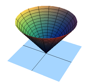
Any $c$-cone divides the hyperbolic space $\mathbb{H}^{3}$ in two parts (see figure 1). One part on the $c$-cone and the other part down the $c$-cone. Using this partition property of the $c$-cones we can state the following Theorem

Theorem B.

Let $E$ be a complete end of revolution in $\mathbb{H}^{3}$. Suppose that the end $E$ is contained on a $c$-cone for some $c>0$. Then, the end $E$ is parabolic.

An other sufficient condition can be provided using horospheres

Theorem C.

Let $E$ be a complete end of revolution in $\mathbb{H}^{3}$. Suppose that the end $E$ is contained on the horosphere $\{x_{3}=z\}$ for some $z>0$. Then, the end $E$ is parabolic.

By using the above Theorem we can characterize the conformal type of ends of revolution immersed inside of a compact set of the hyperbolic space.

Corollary D.

Let $E$ be a complete end of revolution in $\mathbb{H}^{3}$ contained in a compact set of $\mathbb{H}^{3}$. Then, $E$ is a parabolic end.

Moreover, theorem C allow us to know that complete non-parabolic ends of revolution in $\mathbb{H}^{3}$ approaches to the $\{x_{3}=0\}$ plane.

Corollary E.

Let $E$ be a complete and non-parabolic end of revolution in $\mathbb{H}^{3}$. Then,

$$\inf_{p\in E}x_{3}(p)=0.$$

The conformal type of a surface is related with the transcience or recurrence of the Brownian motion. The simplest way to construct Brownian motion on a surface is to construct first the heat kernel which will serve as the density of the transition probability.

Given a surface $\Sigma$ with Laplacian $\triangle$, the heat kernel on $\Sigma$ is a function $p(t,x,y)$ on $(0,\infty)\times\Sigma\times\Sigma$ which is the minimal positive fundamental solution to the heat equation

(1.3) $$\frac{\partial v}{\partial t}=\triangle v.$$

In other words, the Cauchy problem

(1.4) $$\left\{\begin{aligned} \frac{\partial v}{\partial t}&=\triangle v\\ v|_{t=0}&=v_{0}(x)\end{aligned}\right.$$

has solution

(1.5) $$v(x,t)=\int_{\Sigma}p(t,x,y)v_{0}(y)dA(y),$$

where $dA$ is the volume element of $\Sigma$. The Brownian motion on a surface is called recurrent if it visits any open set at arbitrarily large moments of time with probability $1$, and transcient otherwise. The Brownian motion on $\Sigma$ is transcient (see [Gri99, Ahl52, Has60]) if

$$\int_{1}^{\infty}p(t,x,x)dt<\infty$$

Otherwise, the Brownian motion on $\Sigma$ is recurrent. Given a complete and non-compact surface $\Sigma$ and an open precompact set $D\subset\Sigma$, the Brownian motion is recurrent, if and only if, every end of $\Sigma$ with respect to $D$ is parabolic.

Another property of the Brownian motion to be considered in this paper is stochastic completeness. This is a property of a stochastic process to have infinite lifetime. In other words, a process is stochastically complete if the total probability of the particle being found in the state space is constantly equal to $1$. For the Brownian motion this means

(1.6) $$\int_{\Sigma}p(t,x,y)dA(y)=1,$$

for any $t>0$. Namely, the heat kernel is an authentic probability measure. For complete ends of revolution we can state

Theorem F.

Let $\Sigma$ be complete and non-compact surface of finite topological type immersed in $\mathbb{M}^{3}(\kappa)$ with $\kappa\in\mathbb{R}$. Suppose that there exists a compact subset $\Omega\subset\Sigma$ of $\Sigma$ such that every end of $\Sigma$ with respect to $\Omega$ is an end of revolution in $\mathbb{M}^{3}(\kappa)$. Then, $\Sigma$ is stochastically complete.

Hoffman and Meeks proved in [HM90] that a properly immersed minimal surface in $\mathbb{R}^{3}$ disjoint from a plane is a plane. Otherwise stated, if $M$ is a minimal surface properly immersed in $\mathbb{R}^{3}$ and for some $c>0$, $M\cap\{z>c\}\neq\emptyset$, then either $M\cap\{z=c\}\neq\emptyset$, or $M$ is a plane parallel to $\{z=c\}$.

For the hyperbolic space, Rodriguez and Rosenberg proved in [RR98] that every constant mean curvature one surface $M$, properly embedded in a horoball $B\subset\mathbb{H}^{3}$ such that, $M\cap\partial B=\emptyset$, is a horosphere. As a surprising corollary of Theorem F we obtain

Theorem G.

Let $M$ be a complete non-compact surface of revolution properly immersed in $\mathbb{H}^{3}$. Suppose $M\cap B\neq\emptyset$ for some horoball $B\subset\mathbb{H}^{3}$ then,

1. if $M$ has negative sectional curvature, $M\cap\partial B\neq\emptyset$ (otherwise stated, $M$ touches the horosphere $\partial B$).

2. If $M$ has constant non-positive sectional curvature and $M\cap\partial B=\emptyset$, $M$ is a horosphere.

3. If $M$ has constant mean curvature with $\|\vec{H}\|\leq 1$, and $M\cap\partial B=\emptyset$, $M$ is a horosphere.

1.1. outline of the paper

The structure of the paper is as follows

In Section 2 we introduce the definitions of complete end of revolution and we study the relation with the isometry and isotropy group of $\mathbb{M}^{3}(\kappa)$. In Theorem 2.3 and corollary 2.5 we prove that any complete end of revolution can be considered as a submanifold smoothly immersed in $\mathbb{M}^{3}(\kappa)$, and intrinsically each end of revolution is endowed with a warped product metric. Indeed, in Corollary 2.7 is proved that any end of revolution is isometric to a rotationally symmetric $2$-dimensional manifold where a geodesic ball is subtracted. That allow us, by using the well known criteria for parabolicity of rotationally symmetric model manifolds, to obtain Theorem 2.11 and Corollary 2.12 where sufficient and necessary conditions for the parabolicity in terms of the warped function of each end of revolution are provided. In Subsection 2.4 making use of conformal models of $\mathbb{M}^{3}(\kappa)$ we obtain the explicit expressions of such warping functions. With these techniques we can prove Theorems A, B, C, F and G in Sections 3, 4, 5, 6, and 7 respectively. Finally, Section 9 deals with several examples of application of the main Theorems.

2. Preliminaries.

2.1. Isotropy group and Ends of revolution in $\mathbb{M}^{3}(\kappa)$

The only (up to scaling) $3$-dimensional simply connected Riemannian manifolds with a $6$-dimensional isometry group are:

1. The Euclidean space $\mathbb{R}^{3}$ with vanishing curvature.

2. The hyperbolic space $\mathbb{H}^{3}$ with constant sectional curvature on each tangent plane $\kappa_{\mathbb{H}^{3}}=-1$.

3. The sphere $\mathbb{S}^{3}$ with constant sectional curvature on each tangent plane $\kappa_{\mathbb{S}^{3}}=1$.

In this paper we denote by $\mathbb{M}^{3}(\kappa)$, the simply connected space form of constant sectional curvature $\kappa\in\mathbb{R}$. On each point $p\in\mathbb{M}^{3}(\kappa)$ the isotropy subgroup ${\rm stab}(p)$ of the isometry group at $p$ is $O(3)$, actually, see [Pet98] for instance, $\mathbb{R}^{3}=\left(\mathbb{R}^{3}\rtimes O(3)\right)/O(3)$, $\mathbb{S}^{3}=O(4)/O(3)$, $\mathbb{H}^{3}=O(1,3)/O(3)$.

Given a point $p\in\mathbb{M}^{3}(\kappa)$, and an unit vector $v\in T_{p}\mathbb{M}^{3}(\kappa)$. We will denote by $\gamma_{v}$ the geodesic curve starting at $p$ with direction $v$, namely

(2.1) $$\gamma_{v}:\mathbb{R}\to\mathbb{M}^{3}(\kappa),\quad t\to{\rm exp}_{p}(tv).$$

Since any isometry $\varphi\in{\rm stab}(p)$ fixes $p$, the pushfordward $\varphi_{*}:T_{p}\mathbb{M}^{3}(\kappa)\to T_{p}\mathbb{M}^{3}(\kappa)$ induces an automorphism in $T_{p}\mathbb{M}^{3}(\kappa)$. That allow us to obtain the faithful linear isotropy representation $\rho:{\rm stab(p)}\to{\rm GL}(T_{p}\mathbb{M}^{3}(\kappa))$. Let us define

(2.2) $$\mathcal{R}_{v}:=\left\{\varphi\in{\rm stab}(p)\,:\,\varphi_{*}(v)=v,\,{\rm det}(\varphi_{*})=1\right\}.$$

If we choose the orthonormal basis $\{v,E_{1},E_{2}\}$ of $T_{p}\mathbb{M}^{3}(\kappa)$, for any $\varphi\in\mathcal{R}_{v}$ there exists $\theta\in[0,2\pi)$ such that

(2.3) $$\rho(\varphi)=\begin{pmatrix}1&0&0\\ 0&\cos(\theta)&-\sin(\theta)\\ 0&\sin(\theta)&\cos(\theta)\end{pmatrix}$$

Then $\mathcal{R}_{v}$ is a Lie group isomorphic (and diffeormorphic) to $SO(2)$ and can be understood as a rotation along $\gamma_{v}$ because for any $\varphi\in\mathcal{R}_{v}$ we have $\varphi\circ\gamma_{v}(t)=\varphi(\exp(vt))=\exp(\varphi_{*}(v)t)=\exp(vt)=\gamma_{v}(t)$. We can show not only that the points of $\gamma_{v}$ are left fixed by the action of $\mathcal{R}_{v}$, but actually that $\gamma_{v}$ is the set of fixed points of $\mathcal{R}_{v}$. In other words,

Proposition 2.1.

Let $p$ be a point of $\mathbb{M}^{3}(\kappa)$, let $v$ be a vector in $T_{p}\mathbb{M}^{3}(\kappa)$. Then, $\mathcal{R}_{v}$ acts freely on $\mathbb{M}^{3}(\kappa)\setminus(\gamma_{v}(\mathbb{R}))$.

Proof.

We are going to prove that the set of fixed points for $\mathcal{R}_{v}$ is precisely $\gamma_{v}(\mathbb{R})$. Observe that, by using Theorem 5.1 of [Kob95], each connected component of the set of fixed points of $\mathcal{R}_{v}$ is a closed totally geodesic submanifold of $\mathbb{M}^{3}(\kappa)$. Moreover, we can deduce that the set of fixed points has only one connected component $C_{0}\ni p$. Because the connected component $C_{0}$ of the set of fixed points which contains $p$ contains $\gamma_{v}(\mathbb{R})$ as well, and it therefore contains the cut points of $p$ (if $\kappa>0$). But by corollary 5.2 of [Kob95] any other connected component besides $C_{0}$ of the set of fixed points should be formed by cut points of $p$ (which belong to $C_{0}$). Hence, we conclude that the set of fixed points of $\mathcal{R}_{v}$ has only one connected totally geodesic submanifold which contains $p$ and $\gamma_{v}(\mathbb{R})$.

We can prove now that $C_{0}=\gamma_{v}(\mathbb{R})$. Because otherwise since $C_{0}$ is a totally geodesic submanifold, we should have an other vector $v_{2}\in T_{p}\mathbb{M}^{3}(\kappa)$ non proportional to $v$, such that for the geodesic $\gamma_{v_{2}}(t)=\exp_{p}(v_{2}t)$

(2.4) $$\varphi\circ\gamma_{v_{2}}(\mathbb{R})=\gamma_{v_{2}}(\mathbb{R}),\quad\forall\varphi\in\mathcal{R}_{v}.$$

But, since the geodesic curve $\varphi\circ\gamma_{v_{2}}$ at $p$ is tangent to $\varphi_{*}(v_{2})$, that means that

(2.5) $$\varphi_{*}({v_{2}})=v_{2},\quad\forall\varphi\in\mathcal{R}_{v}.$$

Set $v_{2}=v_{2}^{1}v+v_{2}^{2}E_{1}+v_{2}^{2}E_{3}$ the decomposition of $v_{2}$ in the basis $\{v,E_{1},E_{2}\}$, hence by using the representation given in (2.3),

(2.6) $$\begin{pmatrix}1&0&0\\ 0&\cos(\theta)&-\sin(\theta)\\ 0&\sin(\theta)&\cos(\theta)\end{pmatrix}\begin{pmatrix}v_{2}^{1}\\ v_{2}^{2}\\ v_{2}^{3}\end{pmatrix}=\begin{pmatrix}v_{2}^{1}\\ v_{2}^{2}\\ v_{2}^{3}\end{pmatrix},\quad\forall\theta\in[0,2\pi).$$

Namely, $v_{2}^{2}=v_{2}^{3}=0$, and hence, $v_{2}=v_{1}$, but that is a contradiction because we have assumed ${\rm dim}\langle\{v,v_{2}\}\rangle=2$. ∎

The above proposition implies that the canonical projection $\pi:\mathbb{M}^{3}(\kappa)\setminus\gamma_{v}(\mathbb{R})\to(\mathbb{M}^{3}(\kappa)\setminus\gamma_{v}(\mathbb{R}))/\mathcal{R}_{v}$ induces a $\mathcal{R}_{v}$-principal fiber bundle (see [KN96] for instance). Hence, for any $q\in\mathbb{M}^{3}(\kappa)\setminus\gamma_{v}(\mathbb{R})$ the orbit space

(2.7) $$O_{q}:=\left\{\varphi(q)\,:\,\varphi\in\mathcal{R}_{v}\right\}$$

is a smooth submanifold of $\mathbb{M}^{3}(\kappa)\setminus\gamma_{v}(\mathbb{R})$ and $O_{q}\overset{\rm diff.}{\approx}\pi^{-1}(\pi(q))\overset{\rm diff.}{\approx}SO(2)\overset{\rm diff.}{\approx}\mathbb{S}^{1}$. Given $p\in\mathbb{M}^{3}(\kappa)$, $v\in T_{p}\mathbb{M}^{3}(\kappa)$ and $E_{1}\in T_{p}\mathbb{M}^{3}(\kappa)$ with $E_{1}\perp v$, let us define the totally geodesic half-plane $\Pi_{v,E_{1}}^{+}$ by

(2.8) $$\Pi_{v,E_{1}}^{+}:=\{\exp_{p}(vt_{1}+E_{1}t_{2})\,:\,t_{1}\in\mathbb{R},t_{2}>0\}$$

Observe that for any $\varphi\in\mathcal{R}_{v}$,

$$\varphi(\Pi^{+}_{v,E_{1}})=\Pi^{+}_{v,\varphi_{*}(E_{1})}$$

because $\varphi$ is an isometry and hence commutes with the exponential map.

Definition 2.2 (End of revolution).

Given a point $p\in T_{p}\mathbb{M}^{3}(\kappa)$, two perpendicular vectors $v,w\in T_{p}M$ of length $1$, and given a curve $\beta:[0,\infty)\to\Pi_{v,w}^{+}$. An end of revolution $E$ along $\gamma_{v}$ with generating curve $\beta$ is the set

(2.9) $$E:=\left\{\varphi(\beta(t))\,:\,t\in[0,\infty)\,{\rm and}\,\varphi\in\mathcal{R}_{v}\right\}$$

In the following Theorem we shall prove that any end of revolution given by the above definition can be understood as a smooth submanifold with boundary immersed in $\mathbb{M}^{3}(\kappa)$, moreover such an end is intrinsically a warped product.

Theorem 2.3.

Given $p\in\mathbb{M}^{3}(\kappa)$, $v\in T_{p}\mathbb{M}^{3}(\kappa)$. Let $f:\mathbb{S}^{1}\to\mathcal{R}_{v}$ be a diffeomorphism. Then, given a smooth and regular curve $\beta:[0,\infty)\to\Pi^{+}_{v,w}$, for some $w\in T_{p}\mathbb{M}^{3}(\kappa)$ with $\langle w,v\rangle=0$, the map

(2.10) $$\alpha:[0,\infty)\times\mathbb{S}^{1}\to\mathbb{M}^{3}(\kappa),\quad(t,\theta)\to\alpha(t,\theta)=f(\theta)\big{(}\beta(t)\big{)}$$

is an immersion. Moreover, there exists a diffeomorphism $\widetilde{f}:\mathbb{S}_{1}\to\mathbb{S}_{1}$ and a positive function $w:\mathbb{R}^{1}\to\mathbb{R}^{1}$ such that

(2.11) $$\alpha^{*}(g_{\mathbb{M}^{3}(\kappa)})=\|\dot{\beta}\circ\pi_{1}\|^{2}\pi_{1}^{*}g_{\mathbb{R}^{1}}+\left(w\circ\pi_{1}\right)^{2}\left(\widetilde{f}\circ\pi_{2}\right)^{*}g_{\mathbb{S}_{1}}$$

where $\pi_{1}$ and $\pi_{2}$ are the projections

$$\pi_{1}:[0,\infty)\times\mathbb{S}_{1}\to[0,\infty),\quad\pi_{2}:[0,\infty)\times\mathbb{S}_{1}\to\mathbb{S}_{1}$$

and $g_{\mathbb{R}^{1}}$, $g_{\mathbb{S}_{1}}$ are the canonical metrics of $\mathbb{R}^{1}$ and $\mathbb{S}_{1}$ respectively.

Proof.

First of all we have to prove that ${\rm rank}(\alpha_{*})=2$. Given $(t_{0},\theta_{0})\in[0,\infty)\times\mathbb{S}_{1}$, the tangent space $T_{(t_{0},\theta_{0})}[0,\infty)\times\mathbb{S}_{1}$ can be decomposed as

(2.12) $$T_{(t_{0},\theta_{0})}[0,\infty)\times\mathbb{S}_{1}=T_{t_{0}}[0,\infty)\,\oplus\,T_{\theta_{0}}\mathbb{S}_{1}.$$

For any $x\in T_{t_{0}}\mathbb{R}^{1}$, $\alpha_{*}(x)$ is tangent to the plane $\Pi^{+}_{v,f(\theta_{0})_{*}(w)}$, because

(2.13) $$\alpha_{*}(x)= \left.{\frac{d}{dt}}\alpha(t_{0}+xt,\theta_{0})\right|_{t=0}=\left.{\frac{d}{dt}}f(\theta_{0})\left(\beta(t_{0}+xt)\right)\right|_{t=0}$$

and since $\beta$ is a curve in $\Pi^{+}_{v,w}$, then $f(\theta_{0})\beta$ is a curve in $\Pi^{+}_{v,f(\theta_{0})_{*}(w)}$. Moreover,

$$\alpha_{*}(x)=f(\theta_{0})_{*}\left(x\dot{\beta}(t_{0})\right)$$

then $\alpha_{*}(x)\neq 0$ if $x\neq 0$ because the generating curve $\beta$ is regular ($\dot{\beta}\neq 0$). When we consider $y\in T_{\theta_{0}}\mathbb{S}_{1}$, then $\alpha_{*}(y)$ is tangent to the orbit space $O_{\alpha(t_{0},\theta_{0})}$ because for $\gamma:(-\epsilon,\epsilon)\to\mathbb{S}^{1}$, with $\gamma(0)=\theta_{0},\,\dot{\gamma}(0)=y$,

(2.14) $$\alpha_{*}(y)= \left.{\frac{d}{dt}}\alpha(t_{0},\gamma(t))\right|_{t=0}=\left.{\frac{d}{dt}}f(\gamma(t))\left(\beta(t_{0})\right)\right|_{t=0}\in T_{\alpha(\theta_{0},t_{0})}O_{\alpha(\theta_{0},t_{0})}.$$

Moreover, the curve $\gamma$ induces the $1$-parametric subgroup $f(\gamma(t))=\exp(f_{*}(y)t)f(\theta_{0})$ and its action induces a never vanishing vector on $\alpha(t_{0},\theta_{0})$ whenever $y\neq 0$ because the action of $\mathcal{R}_{v}$ is freely on $\mathbb{M}^{3}(\kappa)\setminus\gamma_{v}(\mathbb{R})$ (see proposition 4.1 of [KN96]). Then $\varphi$ in an immersion.

In order to deal with the induced metric $\varphi^{*}(g_{\mathbb{M}^{3}(\kappa)})$ observe that by using the decomposition of equation (2.12) we have only three cases

, Suppose $x\in T_{t_{0}}[0,\infty)$ then,

(2.15) $$\alpha^{*}\left(g_{\mathbb{M}^{3}(\kappa)}\right)(x,x)= \left\langle\alpha_{*}(x),\alpha_{*}(x)\right\rangle_{\mathbb{M}^{3}(\kappa)}$$

$$= \left\langle f(\theta_{0})_{*}\left(x\dot{\beta}(t_{0})\right),f(\theta_{0})_{*}\left(x\dot{\beta}(t_{0})\right)\right\rangle_{\mathbb{M}^{3}(\kappa)}$$

$$= \|\dot{\beta}(t_{0})\|^{2}\|x\|^{2}$$

if $x\in T_{t_{0}}[0,\infty)$ and $y\in T_{\theta_{0}}\mathbb{S}_{1}$, then

$$\alpha^{*}\left(g_{\mathbb{M}^{3}(\kappa)}\right)(x,y)=\left\langle\alpha_{*}(x),\alpha_{*}(y)\right\rangle_{\mathbb{M}^{3}(\kappa)}=0$$

because

Proposition 2.4.

The orbit space $O_{\alpha(t_{0},\theta_{0})}$ is perpendicular to $\Pi^{+}_{v,f(\theta_{0})_{*}w}$.

Proof.

Since ${\rm Cut}(p)\cap\left(\mathbb{M}^{3}(\kappa)\setminus\gamma_{v}\left(\mathbb{R}\right)\right)=\emptyset$, for any $q\in\mathbb{M}^{3}(\kappa)\setminus\gamma_{v}(\mathbb{R})$ we have a well defined

(2.16) $$v(q):=\exp_{p}^{-1}(q).$$

To show that $\Pi^{+}_{v,f(\theta_{0})_{*}w}$ is perpendicular to $O_{\alpha(t_{0},\theta_{0})}$ let us consider the following basis $\{{\exp_{p}}_{*}(v),{\exp_{p}}_{*}(W),{\exp_{p}}_{*}(\nu)\}$ of $T_{\alpha(t_{0},\theta_{0})}\mathbb{M}^{3}(\kappa)$, where here we have used $W:=f(\theta_{0})_{*}(w)$ in order to simplify the notation, and $\{v,W,\nu\}$ is an orthonormal basis of $T_{p}\mathbb{M}^{3}(\kappa)$ and ${\exp_{p}}_{*}$ is the differential of the exponential map, namely

(2.17) $${\exp_{p}}_{*}(v) =\left.\frac{d}{dt}\exp_{p}\left(v(\alpha(t_{0},\theta_{0}))+vt\right)\right|_{t=0}$$

$${\exp_{p}}_{*}(W) =\left.\frac{d}{dt}\exp_{p}\left(v(\alpha(t_{0},\theta_{0}))+Wt\right)\right|_{t=0}$$

$${\exp_{p}}_{*}(\nu) =\left.\frac{d}{dt}\exp_{p}\left(v(\alpha(t_{0},\theta_{0}))+\nu t\right)\right|_{t=0}$$

hence, ${\exp_{p}}_{*}(v)$ and ${\exp_{p}}_{*}(W)$ are tangent to $\Pi^{+}_{v,W}$ and moreover, by using the Gauss lemma (see [dC92]), ${\exp_{p}}_{*}(\nu)\perp\Pi^{+}_{v,W}$ and $\{{\exp_{p}}_{*}(v),{\exp_{p}}_{*}(W),{\exp_{p}}_{*}(\nu)\}$ is an orthonormal basis of $T_{\alpha(t_{0},\theta_{0})}\mathbb{M}^{3}(\kappa)$. Now, let us consider the following two functions

$$f_{1}:\mathbb{M}^{3}(\kappa)\setminus\gamma_{v}\left(\mathbb{R}\right)\to\mathbb{R},\quad f_{1}(x)=\langle\exp_{p}^{-1}(x),\exp_{p}^{-1}(x)\rangle$$

$$f_{2}:\mathbb{M}^{3}(\kappa)\setminus\gamma_{v}\left(\mathbb{R}\right)\to\mathbb{R},\quad f_{2}(x)=\langle v,\exp_{p}^{-1}(x)\rangle$$

since for any $\varphi\in\mathcal{R}_{v}$,

$$f_{1}(\varphi(x))= \langle\exp_{p}^{-1}\varphi(x),\exp_{p}^{-1}\varphi(x)\rangle$$

$$= \langle\varphi_{*}\exp_{p}^{-1}(x),\varphi_{*}\exp_{p}^{-1}\varphi(x)\rangle=\langle\exp_{p}^{-1}(x),\exp_{p}^{-1}(x)\rangle$$

$$= f_{1}(x)$$

$${\rm and},$$

$$f_{2}(\varphi(x))= \langle v,\exp_{p}^{-1}(\varphi(x))\rangle=\langle v,\varphi_{*}\exp_{p}^{-1}(x)\rangle$$

$$= \langle\varphi_{*}v,\varphi_{*}\exp_{p}^{-1}(x)\rangle=\langle v,\exp_{p}^{-1}(x)\rangle$$

$$= f_{2}(x)$$

then, $O_{\alpha(t_{0},\theta_{0})}$ is perpendicular to $\nabla f_{1}$ and $\nabla f_{2}$. Now, we are going to show that $\nabla f_{1}$ and $\nabla f_{2}$ span $T_{\alpha(t_{0},\theta_{0})}\Pi^{+}_{u,W}$. Set $u\in T_{p}\mathbb{M}^{3}(\kappa)$, and consider the curve

(2.18) $$\beta(t)=\exp_{p}(v(\alpha(t_{0},\theta_{0}))+ut)$$

hence, $\beta(0)=\alpha(t_{0},\theta_{0})$ and $\dot{\beta}(0)={\exp_{p}}_{*}(u)$. Moreover

(2.19) $$\langle\dot{\beta}(0),\nabla f_{1}\rangle= \frac{d}{dt}\left.f_{1}\left(\beta\left(t\right)\right)\right|_{t=0}=\frac{d}{dt}\left.\left|v(\alpha(t_{0},\theta_{0}))+ut\right|^{2}\right|_{t=0}=2\langle u,v(\alpha(t_{0},\theta_{0}))\rangle.$$

$$\langle\dot{\beta}(0),\nabla f_{2}\rangle= \frac{d}{dt}\left.f_{2}\left(\beta\left(t\right)\right)\right|_{t=0}=\frac{d}{dt}\left.\langle v(\alpha(t_{0},\theta_{0}))+ut,v\rangle\right|_{t=0}=\langle u,v\rangle.$$

Then, when we focus on the basis $\{{\exp_{p}}_{*}(v),{\exp_{p}}_{*}(W),{\exp_{p}}_{*}(\nu)\}$ of $T_{\alpha(t_{0},\theta_{0})}\mathbb{M}^{3}(\kappa)$

(2.20) $$\begin{pmatrix}\nabla f_{1}\\ \nabla f_{2}\end{pmatrix}=\begin{pmatrix}2\langle v,v(\alpha(t_{0},\theta_{0}))\rangle&2\langle v(\alpha(t_{0},\theta_{0})),W\rangle\\ 1&0\end{pmatrix}\cdot\begin{pmatrix}{\exp_{p}}_{*}(v)\\ {\exp_{p}}_{*}(W)\end{pmatrix}$$

Finally, Taking into account that $\alpha(t_{0},\theta_{0})\in\Pi^{+}_{v,W}$ then there exist $t>0$ such that $\langle v(\alpha(t_{0},\theta_{0})),W\rangle=t\neq 0$, therefore

(2.21) $$\langle\{\nabla f_{1},\nabla f_{2}\}\rangle=\langle\{{\exp_{p}}_{*}(v),{\exp_{p}}_{*}(W)\}\rangle=T_{\langle v(\alpha(t_{0},\theta_{0})),W\rangle}\Pi^{+}_{v,W}.$$

∎

Observe in this case that for every $t_{0}$ the map $f_{1}:\mathcal{R}_{v}\to O_{\beta(t_{0})}$ given by $f_{1}(\theta)=\theta\beta(t_{0}),$ defines a diffeoromphism from $\mathcal{R}_{v}$ to $O_{\beta(t_{0})}$. We can pull-back the metric to $O_{\beta(t_{0})}$ (an hence to $\mathcal{R}_{v}$) by using the inclusion $i:O_{\beta(t_{0})}$, in such a way that the $1$-dimensional manifold $O_{\beta(t_{0})}$ with metric tensor $i^{*}(g_{\mathbb{M}^{3}(\kappa)})$ is isometric to the $1$-dimensional manifold $\mathcal{R}_{v}$ with metric tensor $g_{R}=(i\circ f_{1})^{*}(g_{\mathbb{M}^{3}(\kappa)})$. But we are going to show that the metric $g_{R}$ is a left invariant metric on $\mathcal{R}_{v}$. Given $\theta\in\mathcal{R}_{v}$, let $v,w$ be two vectors of $T_{\theta}\mathcal{R}_{v}$, and let $\gamma_{1}$ and $\gamma_{2}$ be two curves such that

$$\gamma_{1}(0)=\gamma_{2}(0)=\theta,\quad\dot{\gamma}_{1}(0)=v,\quad\dot{\gamma}_{2}(0)=w$$

Since $\mathcal{R}_{v}$ acts by isometries,

$$g_{R}({L_{\varphi}}_{*}v,{L_{\varphi}}_{*}w)_{L_{\varphi}(\theta)}= \left\langle\left.\frac{d}{dt}\left(\varphi\gamma_{1}(t)\right)\right|_{t=0},\left.\frac{d}{dt}\left(\varphi\gamma_{2}(t))\right)\right|_{t=0}\right\rangle_{\varphi(\theta(\beta(t_{0})))}$$

$$= \left\langle\varphi^{-1}_{*}\left.\frac{d}{dt}(\varphi\gamma_{1}(t)(q))\right|_{t=0},\varphi^{-1}_{*}\left.\frac{d}{dt}(\varphi\gamma_{2}(t)(q))\right|_{t=0}\right\rangle_{\theta(\beta(t_{0}))}$$

$$= \left\langle\left.\frac{d}{dt}(\varphi^{-1}\varphi\gamma_{1}(t)(q))\right|_{t=0},\frac{d}{dt}(\varphi^{-1}\varphi\gamma_{2}(t)(q))|_{t=0}\right\rangle_{\theta(\beta(t_{0}))}$$

$$= \left\langle\left.\frac{d}{dt}(\gamma_{1}(t)(q))\right|_{t=0},\frac{d}{dt}(\gamma_{2}(t)(q))|_{t=0}\right\rangle_{\theta(\beta(t_{0}))}$$

$$= \langle{f_{1}}_{*}(v),{f_{1}}_{*}(w)\rangle_{\theta(\beta(t_{0}))}=g_{R}(v,w)_{\theta}.$$

But since $\mathcal{R}_{v}$ is isomorphic (and diffeomorphic) to $SO(2)$ with a left-invariant metric, then $g_{R}$ is the round metric up to a scale factor. Hence, $\mathcal{R}_{v}$ is a homotetia of $\mathbb{S}^{1}$ then

(2.22) $$\alpha^{*}\left(g_{\mathbb{M}^{3}(\kappa)}\right)(y,y)= w^{2}(t_{0})(\widetilde{f})^{*}(g_{\mathbb{S}_{1}})\left(y,y\right).$$

for any $y\in T_{\theta_{0}}\mathbb{S}_{1}$. ∎

Corollary 2.5.

Under the assumptions of the above Theorem, can be found a local coordinate system $\{t,\theta\}$ of $[0,\infty)\times\mathbb{S}_{1}$ such that

$$\alpha^{*}(g_{\mathbb{M}}^{3}(\kappa))=dt^{2}+w^{2}(t)d\theta^{2}.$$

2.2. Rotationally symmetric model spaces

Rotationally symmetric model spaces, are generalized manifolds of revolution using warped products. Let us recall here the following definition of a model space.

Definition 2.6 (See [GW79, Gri99, Gri09]).

A $w-$model space $\mathbb{M}_{w}^{n}$ is a simply-connected $n$-dimensional smooth manifold $\mathbb{M}_{w}^{n}$ with a point $o_{w}\in\mathbb{M}_{w}^{n}$ called the center point of the model space such that $\mathbb{M}_{w}^{n}-\{o_{w}\}$ is isometric to a smooth warped product with base $B^{1}=(\,0,\,\Lambda)\,\,\subset\,\mathbb{R}$ (where $\,0<\Lambda\leq\infty$ ), fiber $F^{n-1}=\mathbb{S}^{n-1}_{1}$ (i.e., the unit $(n-1)-$sphere with standard metric), and positive warping function $w:\,(\,0,\,\Lambda\,)\to\mathbb{R}_{+}$. Namely the metric tensor $g_{\mathbb{M}_{w}^{n}}$ is given by:

(2.23) $$g_{\mathbb{M}_{w}^{n}}=r^{*}\left(g_{(\,0,\,\Lambda)}\right)+(w\circ\pi)^{2}\Theta^{*}\left(g_{\mathbb{S}^{n-1}_{1}}\right)\quad,$$

$r:\mathbb{M}_{w}^{n}\to(\,0,\,\Lambda)$ and $\Theta:\mathbb{M}_{w}^{n}\to\mathbb{S}^{n-1}_{1}$ being the projections onto the factors of the warped product, and $g_{(\,0,\,\Lambda)}$ and $g_{\mathbb{S}^{n-1}_{1}}$ the standard metric tensor on the interval and the sphere respectively.

Despite the freedom in the choice of the $w$ function in the above definition, there exist certain restrictions around $r\to 0$. In order to attain $\mathbb{M}_{w}^{n}$, a smooth metric tensor around $o_{w}$, the positive warping function $w$ should hold the following equalities (see [GW79, Pet98]):

(2.24) $$w(0)=0\quad,$$

$$w^{\prime}(0)=1\quad,$$

$$w^{(2k)}(0)=0\quad,$$

where $w^{(2k)}(r)$ are the even derivatives of $w$.

The parameter $\Lambda$ in the above definition is called the radius of the model space. If $\Lambda=\infty$, then $o_{w}$ is a pole of $\mathbb{M}_{w}^{n}$ (i.e., the exponential map $\text{exp}_{o_{w}}:T_{o_{w}}\mathbb{M}_{w}^{n}\to\mathbb{M}_{w}^{n}$ is a diffeomorphism).

Observe that a rotationally symmetric model space $\mathbb{M}_{w}^{n}$ is rotationally symmetric at $o_{w}\in\mathbb{M}^{n}_{w}$ in the sense that the isotropy subgroup at $o_{w}$ of the isometry group is $O(n)$. More commonly, one regards the functions $(r,\Theta)$ as global coordinate functions on $\mathbb{M}_{w}^{n}-\{o_{w}\}$ and the expression of the metric tensor (2.23) is written as $g_{\mathbb{M}_{w}^{n}}=dr^{2}+\left(w(r)\right)^{2}d\Theta^{2}$, where $dr^{2}$ denotes the standard metric on the interval and $d\Theta^{2}$ denotes the standard metric on $\mathbb{S}^{n-1}_{1}$ ( $d\Theta^{2}=g_{\mathbb{S}^{n-1}_{1}}$). In this context, $\{r,\Theta\}$ are called geodesic polar coordinates around $o_{w}$.

In view of the definitions of ends of revolution in $\mathbb{M}^{3}(\kappa)$, Corollary 2.5 and the definition of a rotationally symmetric model manifold we can state.

Corollary 2.7.

Let $E$ be an end of revolution in $\mathbb{M}^{3}(\kappa)$, let $w$ be the warping function given by corollary 2.5. Then for every positive radius $\rho>0$ there exists a $W\in C^{\infty}[0,\infty)$ with

$$W(x)=w(x-\rho),\quad\forall x\geq\rho$$

such that $E$ is isometric to $\mathbb{M}^{2}_{W}\setminus B_{\rho}(o_{W})$ where $B_{\rho}(o_{W})$ is the geodesic ball of radius $\rho$ centered at $o_{W}\in\mathbb{M}_{W}^{2}$.

Proof.

We only have to prove the following lemma

Lemma 2.8.

Given a positive $\rho>0$ and a positive function $w\in C^{\infty}[0,\infty)$, the function can be extended to a function $W\in C^{\infty}[0,\infty)$ such that

$$\left\{\begin{aligned} &W(x)=w(x-\rho),\quad\forall x\geq\rho\\ &W(0)=0\quad,\\ &W^{\prime}(0)=1\quad,\\ &W^{(2k)}(0)=0\quad,\\ &W(x)>0,\quad\forall x>0\quad.\end{aligned}\right.$$

Proof.

We can choose $\epsilon>0$ such that $\epsilon<\rho$. We can define moreover the function $F:[\frac{\epsilon}{2},\epsilon]\cup[\rho,\infty)\to\mathbb{R}_{+}$ given by

$$F(x):=\left\{\begin{array}[]{lcr}x&{\rm if}&\frac{\epsilon}{2}\leq x\leq\epsilon\\ w(x-\rho)&{\rm if}&x\geq\rho.\end{array}\right.$$

Since $F$ is a $C^{\infty}$ function from the closed set $C:=[\frac{\epsilon}{2},\epsilon]\cup[\rho,\infty)$ of $(0,\infty)$ to $\mathbb{R}_{+}$ and $F$ has a continuous extension to $(0,\infty)$, then by using the extension lemma for smooth maps (see Corollary 6.27 of [Lee03]), there exists a $C^{\infty}$ function $\widetilde{F}:\mathbb{R}_{+}\to\mathbb{R}_{+}$ such that $\widetilde{F}_{|C}=F$. Finally we can define the function $W:[0,\infty)\to[0,\infty)$ by

$$W(x):=\left\{\begin{array}[]{lcr}x&{\rm if}&x\leq\rho\\ \widetilde{F}(x)&{\rm if}&x\geq\rho.\end{array}\right.$$

∎

∎

2.3. Recurrence and non explosion of ends of revolution

Conditions for recurrence and non-explosion of the Brownian motion on a Riemannian manifold have been largely studied (see [Gri99] [Ich82a] [Ich82b] [Ahl35], [Nev40] for example). In the particular case of rotationally symmetric model manifolds

Theorem 2.9.

[Gri99] Let $\mathbb{M}_{w}^{n}$ be a model manifold with $\Lambda=\infty$ (so that $\mathbb{M}_{w}^{n}$ is geodesically complete and non-compact). Then $\mathbb{M}_{w}^{n}$ is recurrent if and only if

(2.25) $$\int^{\infty}\frac{dt}{w^{n-1}(t)}=\infty$$

Theorem 2.10.

[Gri99] Let $\mathbb{M}_{w}^{n}$ be a model manifold with $\Lambda=\infty$. Then $\mathbb{M}_{w}^{n}$ is stochastically complete if and only if

(2.26) $$\int^{\infty}\frac{\int_{0}^{t}w^{n-1}(s)ds}{w^{n-1}(t)}dt=\infty$$

Actually (see [GH14] proof of Theorem 1.5) if $\int^{\infty}\frac{\int_{0}^{t}w^{n-1}(s)ds}{w^{n-1}(t)}dt=\infty$ then we can construct a $1$-superharmonic and radial function $v$ in $M\setminus B_{\rho}^{n}(o_{w})$ (that is $-\triangle u+u\geq 0$) such that $v(\rho)=1$, $v^{\prime}(0)=0$, and $v(x)\to\infty$ as $x\to\infty$.

There are sufficient conditions to attain parabolicity for rotationally symmetric model manifolds as well

Theorem 2.11 (see [Gri99]).

Let $\mathbb{M}^{n}_{w}$ be a rotationally symmetric model manifold. Suppose that

$$\int^{\infty}\frac{tdt}{\int_{0}^{t}w(s)ds}=\infty,$$

then $\mathbb{M}^{n}_{w}$ is recurrent.

In view of Corollary 2.7 we can state

Corollary 2.12.

Let $E$ be an end of revolution in $\mathbb{M}^{3}(\kappa)$ isometric to the rotationally symmetric model manifold $\mathbb{M}_{w}^{2}\setminus B_{\rho}(o_{w})$ for some radius $\rho>0$, then $E$ is parabolic if and only if

(2.27) $$\int^{\infty}_{\rho}\frac{dt}{w(t)}=\infty$$

Moreover, if

(2.28) $$\int^{\infty}_{\rho}\frac{\int_{0}^{t}w(s)ds}{w(t)}dt=\infty$$

then, there exist a compact $K\subset E$ and $1$-superharmonic function such that $v(x)\to\infty$ when $x\to\infty$.

We will need moreover the following proposition

Proposition 2.13 (see Theorem 1.3 of [GH14]).

Let $M$ be a connected manifold and $K\subset M$ be a compact set. Assume that there exist a $1$-superharmonic function in $m\setminus K$ such that $v(x)\to\infty$ as $x\to\infty$. Then $M$ is stochastically complete.

2.4. Conformal models of $\mathbb{M}^{3}(\kappa)$ and ends of revolution

The real space forms $\mathbb{R}^{3}$, $\mathbb{S}^{3}$ and $\mathbb{H}^{3}$ can be defined as the 3-dimensional real space forms $\mathbb{M}^{3}(\kappa)$ of constant sectional curvature $\kappa=0,1$ and $-1$ respectively. By using Corollary 2.7 each end of revolution is isometric to a rotationally symmetric model manifold $\mathbb{M}_{w}^{2}\setminus B_{\rho}(o_{w})$ where we have subtracted some ball $B_{\rho}(o_{w})$. The proof of the Theorems A,B,F makes use of Corollary 2.12 were is related the conformal type and the stochastic completeness with the properties of the warping function $w$. Hence, in order to apply Corollary 2.12 we need to know the warping function $w$ of such rotationally symmetric models $\mathbb{M}_{w}^{2}$.

From now on we are going to work with conformal models of $\mathbb{M}^{3}(\kappa)$ (see [Lee97]), namely

(2.29) $$\mathbb{R}^{3} :=\left\{(x_{1},x_{2},x_{3})\in\mathbb{R}^{3}\,:\,g=dx_{1}^{2}+dx_{2}^{2}+dx_{3}^{2}\right\}$$

$$\mathbb{H}^{3} :=\left\{(x_{1},x_{2},x_{3})\in\mathbb{R}^{3},\,x_{3}>0\,:\,g_{-1}=\frac{1}{x_{3}^{2}}\left(dx_{1}^{2}+dx_{2}^{2}+dx_{3}^{2}\right)\right\}$$

$$\mathbb{S}^{3}-\{N\} :=\left\{(x_{1},x_{2},x_{3})\in\mathbb{R}^{3}\,:\,g_{1}=\frac{4\left(dx_{1}^{2}+dx_{2}^{2}+dx_{3}^{2}\right)}{\left(1+x_{1}^{2}+x_{2}^{2}+x_{3}^{2}\right)^{2}}\right\}$$

Indeed, $\mathbb{M}^{3}(\kappa)$ can be seen as $\mathbb{R}^{3}$ endowed with a conformal metric:

(2.30) $$\mathbb{M}^{3}(\kappa):=\left\{(x_{1},x_{2},x_{3})\in\mathbb{R}^{3}:g_{\kappa}=\eta_{\kappa}(x)\cdot g\right\}$$

with

(2.31) $$\eta_{\kappa}(x):=\left\{\begin{array}[]{lcl}\frac{1}{x_{3}^{2}}&\text{ if }&\kappa=-1\\ 1&\text{ if }&\kappa=0\\ \frac{4}{\left(1+x_{1}^{2}+x_{2}^{2}+x_{3}^{2}\right)^{2}}&\text{ if }&\kappa=1\end{array}\right.$$

Observe that $x_{3}$-axis in such models is a geodesic curve. And for any point $x\in\mathbb{M}^{3}(\kappa)$, with $x=(0,0,x_{3})$,

$$R_{\theta}:=\left(\begin{array}[]{ccc}\cos\theta&-\sin\theta&0\\ \sin\theta&\cos\theta&0\\ 0&0&1\end{array}\right)$$

is the subgroup of the isotropy group of $x$ such that the geodesic curve $\gamma(t)=(0,0,x_{3}+t)$ remains fixed under the action of $R_{\theta}$. Taking into account moreover that the $(x_{1},x_{3})$-plane is a totally geodesic submanifold we can construct ends of revolution in $\mathbb{M}^{3}(\kappa)$ in the following way:

Definition 2.14.

Let $\Gamma$ be a regular curve in the $(x_{1},x_{3})$-plane. We define an end of revolution $E:=R_{\theta}\Gamma$ as the action of $R_{\theta}$ to curve $\Gamma$. Here we parameterize the curve $\Gamma$ as

$$\Gamma:=\gamma(s)=(\gamma_{1}(s),0,\gamma_{2}(s))$$

The end of revolution can be parametrized therefore as

(2.32) $$E:=f(s,\theta)=\left(\gamma_{1}(s)\cos\theta,\gamma_{1}(s)\sin\theta,\gamma_{2}(s)\right)$$

Remark a.

Note that by using Theorem 2.3 if we impose $\gamma_{1}(s)>0$, the map given in formula (2.32) can be considered as an immersion from $[0,\infty)\times\mathbb{S}_{1}$ to $\mathbb{M}^{3}(\kappa)$.

Lets recall that every regular curve admits a reparametrization by arc length. Then, from the metrics defined in (2.29) and considering that the parametrization of the immersion given in (2.32) satisfies $\|f_{s}(s,\theta)\|^{2}=1$, it is easy to see that the metric inherited by the end from each ambient space $\mathbb{M}^{3}(\kappa)$ can be written as

(2.33) $$g_{E}=ds^{2}+w_{\kappa}^{2}(s)d\theta^{2}$$

where

(2.34) $$w_{\kappa}(s):=\left\{\begin{array}[]{lcl}\frac{\gamma_{1}(s)}{\gamma_{2}(s)}&\text{ if }&\kappa=-1\\ \gamma_{1}(s)&\text{ if }&\kappa=0\\ \frac{2\gamma_{1}(s)}{1+\gamma_{1}^{2}(s)+\gamma_{2}^{2}(s)}&\text{ if }&\kappa=1\end{array}\right.$$

Indeed, taking $\eta_{\kappa}(s)$ from definition (2.31) we can rewrite the inherited metric as

(2.35) $$g_{E}=ds^{2}+\eta_{\kappa}^{2}(s)w_{0}^{2}(s)d\theta^{2}$$

Hence we can summarize with the following proposition

Proposition 2.15.

Let $E$ be an end of revolution of $\mathbb{M}^{3}(\kappa)$ parametrizated by

$$f(s,\theta)=\left(\gamma_{1}(s)\cos\theta,\gamma_{1}(s)\sin\theta,\gamma_{2}(s)\right)$$

with $s\in[0,\infty)$, $\theta\in[0,2\pi]$. Suppose $\gamma(s)=\left(\gamma_{1}(s),0,\gamma_{2}(s)\right)$ is a regular curve parametrized by arc length and suppose moreover that $\gamma_{1}>0$. Then, for $\rho>0$, $E$ is isometric to $\mathbb{M}_{w}^{2}\setminus B_{\rho}(o_{w})$, where $\mathbb{M}_{w}^{2}$ is the rotationally symmetric model space given by warping function $w$ satisfying

(2.36) $$\left\{\begin{array}[]{lcl}w(t+\rho)=w_{\kappa}(t)&\text{ for }&t\geq 0\\ w(0)=0&&\\ w^{\prime}(0)=0&&\\ w^{(2k)}(0)=0&&\\ \end{array}\right.$$

with $w_{\kappa}$ given in definition (2.34). Hence by applying corollary 2.12 $E$ is parabolic if and only if

(2.37) $$\int^{\infty}_{\rho}\frac{dt}{w(t)}=\int^{\infty}_{0}\frac{ds}{w_{\kappa}(s)}=\infty$$

and if

(2.38) $$\int^{\infty}_{\rho}\frac{\int_{0}^{t}w(s)ds}{w(t)}dt=\int_{0}^{\infty}\frac{\int_{0}^{\rho}w(s)ds+\int_{0}^{t}w_{\kappa}(s)ds}{w_{\kappa}(t)}dt=\infty$$

then, there exist a compact set $K\subset E$ and $1$-superharmonic function such that $v(x)\to\infty$ when $x\to\infty$.

From Theorem 2.11 we can state

Corollary 2.16.

Let $E$ be an end of revolution in $\mathbb{M}^{3}(\kappa)$ if

$$\int^{\infty}\frac{tdt}{\int_{0}^{t}w_{\kappa}(s)ds}=\infty,$$

then $E$ is parabolic.

3. Proof of Theorem A

Theorem A states that any end of revolution in $\mathbb{R}^{3}$ or in $\mathbb{S}^{3}$ is a parabolic end. Here we split the prove in these two settings

3.1. End immersed in $\mathbb{R}^{3}$

Proof.

Lets recall that the generating curve $\gamma(s)$ was parameterized by its arc length. This implies that $(\dot{\gamma}_{1})^{2}(s)\leq 1$. Using definition (2.34) we find this equivalent to

$$-1\leq\dot{w}_{0}(t)\leq 1$$

Integrating the latter we obtain

$$-t\leq w_{0}(t)-w_{0}(0)\leq t$$

and thus $w_{0}(t)\leq t+w_{0}(0)$. By using the criterion for parabolicity given by proposition 2.15

(3.1) $$\int^{\infty}_{0}\frac{1}{w_{0}(s)}ds=\lim_{R\to\infty}\int_{0}^{R}\frac{1}{w_{0}(s)}ds\geq\lim_{R\to\infty}\int_{0}^{R}\frac{1}{t+w_{0}(0)}dt=\infty.$$

Which means that each complete end of revolution $E$, when immersed in $\mathbb{R}^{3}$, is of parabolic conformal type independently of the curve $\gamma(s)$. ∎

3.2. End immersed in $\mathbb{S}^{3}$

Proof.

Applying the criterion for parabolicity at proposition 2.15 and the expression (2.34) for the function $w_{1}(s)$ we have to prove that the following integral is divergent

$$\int^{\infty}_{0}\frac{1}{w_{1}(s)}ds=\int^{\infty}_{0}\frac{1+\gamma_{1}^{2}(s)+\gamma_{2}^{2}(s)}{2\gamma_{1}(s)}ds.$$

For any $\varepsilon>0$, we can split the interval where we integrate ($I=[0,\infty)$) in two parts: $I_{+}=\{t\in I:\gamma_{1}(t)\geq\varepsilon\}$ and $I_{-}=\{t\in I:\gamma_{1}(t)<\varepsilon\}$, such that $I_{+}\cup I_{-}=I$, $I_{+}\cap I_{-}=\emptyset$ and since $\int_{I}dx=\infty$, thus $\int_{I_{+}}dx+\int_{I_{-}}dx=\infty$. Then we have two cases.

, so as we have seen:

$$\int_{I}\frac{1}{w_{1}(s)}ds\geq\int_{I_{+}}\frac{1+\gamma_{1}^{2}(s)+\gamma_{2}^{2}(s)}{2\gamma_{1}(s)}ds\geq\frac{1}{2}\int_{I_{+}}\gamma_{1}(s)ds\geq\frac{1}{2}\varepsilon\int_{I_{+}}ds=\infty$$

, then

$$\int_{I}\frac{1}{w_{1}(s)}ds\geq \int_{I_{-}}\frac{1+\gamma_{1}^{2}(s)+\gamma_{2}^{2}(s)}{2\gamma_{1}(s)}ds\geq\int_{I_{-}}\frac{1}{2\gamma_{1}(s)}ds$$

$$\geq \int_{I_{-}}\frac{1}{2\varepsilon}ds\geq\frac{1}{2\varepsilon}\int_{I_{-}}ds=\infty$$

Which means again that the end is parabolic independently of the curve $\gamma(s)$.∎

4. Proof Theorem B

Theorem B states that every end of revolution on a $c$-cone is a parabolic end. Observe that if the end is on a $c$-cone then the generating profile curve $\gamma(s)=(\gamma_{1}(s),0,\gamma_{2}(s))$ satisfies

(4.1) $$\frac{\gamma_{2}(s)}{\gamma_{1}(s)}\geq c.$$

Substituting the function $w_{-1}(s)$ given by (2.34) in the criterion for parabolicity given in proposition (2.15), we get that the end of the surface will be parabolic because

$$\int^{\infty}_{0}\frac{1}{w_{-1}(s)}ds=\int^{\infty}_{0}\frac{\gamma_{2}(s)}{\gamma_{1}(s)}ds\geq\int^{\infty}_{0}c\,ds=\infty.$$

This finishes the proof of Theorem B. However, we can state something more general. let us denote $I_{+}:=\{t\in I:\frac{\gamma_{2}(t)}{\gamma_{1}(t)}\geq c\}$ and $I_{-}:=\{t\in I:\frac{\gamma_{2}(t)}{\gamma_{1}(t)}<c\}$. Then,

$$\int_{I}\frac{1}{w_{-1}(s)}ds=\int_{I_{+}}\frac{\gamma_{2}(s)}{\gamma_{1}(s)}ds+\int_{I_{-}}\frac{\gamma_{2}(s)}{\gamma_{1}(s)}ds\geq c\int_{I_{+}}ds+\int_{I_{-}}\frac{\gamma_{2}(s)}{\gamma_{1}(s)}ds.$$

Hence if $\int_{I_{+}}ds=\infty$, the end will still be parabolic. Therefore

Theorem 4.1.

Let $E$ be an end of revolution in $\mathbb{H}^{3}$. Suppose that the generating curve of $E$ satisfies

$$\int_{I_{+}}ds=\infty.$$

Then, the end is parabolic.

5. Proof of Theorem C

The first step to prove Theorem C is to prove previously the following proposition

Proposition 5.1.

Let $E$ be a complete end of revolution immersed in $\mathbb{H}^{3}$. Suppose that $E$ is a non-parabolic end, and $\gamma:[0,\infty)\to\mathbb{H}^{3}$ is the profile curve of $E$ parametrized by arc length in the half space model of the hyperbolic space given by

$$\gamma(s)=(\gamma_{1}(s),0,\gamma_{2}(s))$$

then

$$\sup_{s\in[0,\infty)}\gamma_{1}(s)<\infty,$$

Proof.

Since $\gamma_{1}$ is a positive and smooth function, then,

(5.1) $$\log\gamma_{1}(s)-\log\gamma_{1}(0)=\int_{0}^{s}\frac{d}{dt}\left(\log\gamma_{1}(t)\right)dt=\int_{0}^{s}\frac{\dot{\gamma}_{1}(t)}{\gamma_{1}(t)}dt.$$

But taking into account that $\gamma$ is parametrizated by arc length, namely,

$$\frac{(\dot{\gamma}_{1}(s))^{2}+(\dot{\gamma}_{2}(s))^{2}}{(\gamma_{2}(s))^{2}}=1,$$

then,

$$\dot{\gamma}_{1}(s)\leq|\dot{\gamma}_{1}(s)|\leq\gamma_{2}(s)$$

and hence, inequality (5.1) can be rewritten as

(5.2) $$\log\gamma_{1}(s)-\log\gamma_{1}(0)\leq\int_{0}^{s}\frac{\gamma_{2}(t)}{\gamma_{1}(t)}dt$$

By using the function $w_{-1}(s)$ given by (2.34) in the criterion for parabolicity given in proposition 2.15

(5.3) $$\int^{\infty}_{0}\frac{1}{w_{-1}(s)}ds=\int^{\infty}_{0}\frac{\gamma_{2}(s)}{\gamma_{1}(s)}ds<\infty.$$

And hence,

(5.4) $$\log\gamma_{1}(s)-\log\gamma_{1}(0)<\int_{0}^{\infty}\frac{\gamma_{2}(t)}{\gamma_{1}(t)}dt<\infty.$$

∎

Proof of Theorem C.

Theorem C states that any complete end of revolution contained on a horosphere $\{x_{3}=z\}$ is a parabolic end. Since the end is on the horosphere $\{x_{3}=z\}$ then

(5.5) $$\int^{\infty}_{0}\frac{1}{w_{-1}(s)}ds=\int^{\infty}_{0}\frac{\gamma_{2}(s)}{\gamma_{1}(s)}ds\geq z\int^{\infty}_{0}\frac{1}{\gamma_{1}(s)}ds.$$

Hence the end is parabolic because otherwise if we suppose that $E$ is non-parabolic, by using proposition 5.1,

(5.6) $$\int^{\infty}_{0}\frac{1}{w_{-1}(s)}ds\geq z\int^{\infty}_{0}\frac{1}{\sup_{s\in[0,\infty)}\gamma_{1}(s)}ds=\infty.$$

Then by using the criterion for parabolicity given in proposition 2.15 the end $E$ is parabolic (contradiction). ∎

6. Proof of Theorem F

Recall that Theorem F states

Theorem.

Let $\Sigma$ be complete and non-compact surface of finite topological type immersed in $\mathbb{M}^{3}(\kappa)$ with $\kappa\in\mathbb{R}$. Suppose that there exists a compact subset $\Omega\subset\Sigma$ of $\Sigma$ such that every end of $\Sigma$ with respect to $\Omega$ is an end of revolution in $\mathbb{M}^{3}(\kappa)$. Then, $\Sigma$ is stochastically complete.

Proof.

When $\Sigma$ is immersed in $\mathbb{R}^{3}$ or in $\mathbb{S}^{3}$ the stochastic completeness of its ends is straight forward according that every parabolic surface is stochastically complete (see [Gri99]for instance). For surfaces $\Sigma$ in $\mathbb{H}^{3}$ such that every of its ends with respect to some compact $\Omega\subset\Sigma$ is an end of revolution in $\mathbb{H}^{3}$, we are going to show that there exist a $1$-superharmonic function satisfying the hypothesis of proposition 2.13 (and hence $\Sigma$ is stochastically complete). In order to construct such a function we are going to use the following proposition

Proposition 6.1.

Let $E$ be an end of revolution in $\mathbb{H}^{3}$, then, there exist a compact set $K\subset E$ and $1$-superharmonic function such that $v(x)\to\infty$ when $x\to\infty$.

Proof.

From (2.34) we have that

$$w_{-1}(s)=\frac{\gamma_{1}(s)}{\gamma_{2}(s)}$$

hence,

$$\frac{\dot{w}_{-1}(s)}{w_{-1}(s)}=\frac{\dot{\gamma}_{1}(s)}{\gamma_{1}(s)}-\frac{\dot{\gamma}_{2}(s)}{\gamma_{2}(s)}$$

From the condition that $\gamma(s)$ is parameterized by arc length we have that $|\dot{\gamma}_{1}(s)|\leq\gamma_{2}(s)$ and $|\dot{\gamma}_{2}(s)|\leq\gamma_{2}(s)$. Then

(6.1) $$\frac{\dot{w}_{-1}(s)}{w_{-1}(s)}\leq\frac{\gamma_{2}(s)}{\gamma_{1}(s)}+\frac{\gamma_{2}(s)}{\gamma_{2}(s)}=\frac{1}{w_{-1}(s)}+1$$

For any $c>0$ we can now split the interval $I=[0,\infty)$ in two parts, $I=I_{+}\cup I_{-}$ such that $I_{+}:=\{s\in\mathbb{R}:\frac{\gamma_{2}(s)}{\gamma_{1}(s)}\geq c\}$ and $I_{-}=\{s\in\mathbb{R}:\frac{\gamma_{2}(s)}{\gamma_{1}(s)}<c\}$. With $I_{+}\cap I_{-}=\emptyset$, $\int_{I}ds=\int_{I_{+}}ds+\int_{I_{-}}ds=\infty$.We have again two cases:

Then

$$\int^{\infty}\frac{1}{w_{-1}(s)}ds =\int_{I_{+}}\frac{1}{w_{-1}(s)}ds+\int_{I_{-}}\frac{1}{w_{-1}(s)}ds\geq\int_{I_{+}}cds+\int_{I_{-}}\frac{1}{w_{-1}(s)}ds$$

$$=c\cdot\int_{I_{+}}ds+\int_{I_{-}}\frac{1}{w_{-1}(s)}ds=\infty$$

Hence, by applying corollary 2.12 the proposition follows.

for $s>\rho$,

(6.2) $$w(s)-w(\rho) =\int_{\rho}^{s}\dot{w}(r)dr=\int_{[\rho,s]\cap I_{+}}\dot{w}(r)dr+\int_{[\rho,s]\cap I_{-}}\dot{w}(r)dr$$

$$<\int_{[\rho,s]\cap I_{+}}w^{\prime}(r)dr+(1+c)\int_{[\rho,s]\cap I_{-}}w(r)dr$$

where we have considered that in $I_{-}$ by using inequality (6.1), $\dot{w}(r)<(1+c)\,w(r)$. Then,

$$1<\frac{w(\rho)}{w(s)}+\frac{\int_{[\rho,s]\cap I_{+}}w^{\prime}(r)dr}{w(s)}+\frac{(1+c)\int_{[\rho,s]\cap I_{-}}w(r)dr}{w(s)}.$$

Integrating in $[\rho,R]$,

(6.3) $$R-\rho <\int^{R}_{\rho}\frac{w(\rho)}{w(s)}ds+\int^{R}_{\rho}\frac{\int_{[\rho,s]\cap I_{+}}w^{\prime}(r)dr}{w(s)}ds+\int^{R}_{\rho}\frac{(1+c)\int_{[\rho,s]\cap I_{-}}w(r)dr}{w(s)}ds$$

$$\leq\int^{\infty}_{\rho}\frac{w(\rho)}{w(s)}ds+\int^{\infty}_{\rho}\frac{\int_{[\rho,s]\cap I_{+}}w^{\prime}(r)dr}{w(s)}ds+(1+c)\int^{\infty}_{\rho}\frac{\int_{\rho}^{s}w(r)dr}{w(s)}ds$$

taking into account that by using inequality (6.1), $w^{\prime}(r)\leq 1+w(r)$, then for any $R>\rho$,

(6.4) $$R-\rho< w(\rho)\int^{\infty}_{\rho}\frac{1}{w(s)}ds+\int^{\infty}_{\rho}\frac{\int_{[\rho,s]\cap I_{+}}(1+w(r))dr}{w(s)}ds$$

$$+(1+c)\int^{\infty}_{\rho}\frac{\int_{\rho}^{s}w(r)dr}{w(s)}ds$$

$$\leq \left(w(\rho)+\int_{I_{+}}dr\right)\int^{\infty}\frac{1}{w(s)}ds+(2+c)\int^{\infty}_{\rho}\frac{\int_{\rho}^{s}w(r)dr}{w(s)}ds.$$

Letting now $R$ tent to infinity we conclude that or

$$\int^{\infty}_{0}\frac{1}{w(s)}ds=\infty$$

or

$$\int^{\infty}_{\rho}\frac{\int_{\rho}^{s}w(r)dr}{w(s)}ds.$$

But in any case the proposition follows by using proposition 2.15. ∎

Now by applying the above proposition in each connected component of $\Sigma\setminus\Omega$ (call them $\{E_{i}\}$) there exist a compact set $K_{i}\subset E_{i}$ and a $1$-superharmonic function $v_{i}$ in $E_{i}\setminus K_{i}$ such that $v_{i}(x)\to\infty$ as $x\to\infty$. Defining a compact $C$ as

$$C=\Omega\cup_{i}K_{i}$$

and the function $\widetilde{v}:\Sigma\setminus C\to\mathbb{R}$ by

$$\widetilde{v}(x):=v_{i}(x),\quad\text{ if }x\in E_{i}.$$

we conclude that $\widetilde{v}$ is $1$-superharmonic function in $\Sigma\setminus C$ and $\widetilde{v}(x)\to\infty$ as $x\to\infty$. Hence, by applying proposition 2.15 the Corollary is proved. ∎

7. Proof of Theorem G

Recently in [BdLPS13] is proved that any non-compact surface $\Sigma$ which is stochastically and geodesically complete, properly immersed into a horoball of the hyperbolic space $B\subset\mathbb{H}^{3}$ has

(7.1) $$\sup_{x\in\Sigma}\|\vec{H}\|\geq 1,$$

and

(7.2) $$\sup_{x\in\Sigma}K_{G}\geq 0.$$

Hence, there are no surfaces of revolution which are negatively curved and properly immersed into an horoball (statement (1) of Theorem G). Moreover, if $\Sigma$ is a cmc-surface, $\Sigma$ is a cmc one surface and therefore by using [RR98] is a horosphere. On the other hand if $\Sigma$ has constant non-positive sectional curvature, then $K_{G}=0$. But the only complete flat surface contained in a horoball is the horosphere (see Theorem 3 of [GMM00] for instance).

8. Movement of the centroid of a curve in $\mathbb{H}^{2}$ and its applications to the conformal type

Given a regular curve $\gamma:[0,\infty)\to\mathbb{H}^{2}\subset\mathbb{H}^{3}$, parametrized by arc length in the half space model of the hyperbolic space

$$\gamma(s)=(\gamma_{1}(s),0,\gamma_{2}(s)),\quad{\rm with}\quad\gamma_{1}>0\text{ and }\gamma_{2}>0$$

We shall say that the segment $\gamma([0,s])$ has centroid $x_{g}(\gamma([0,s]))$, given by

$$x_{g}(\gamma([0,s])):=\frac{\int_{0}^{s}w_{-1}(t)dt}{s}$$

Theorem 8.1.

Suppose that the centroid of a regular curve $\gamma:[0,\infty)\to\mathbb{H}^{2}$ satisfies

$$x_{g}(\gamma[0,s])\leq C\,s$$

for some $C>0$ and any $s\geq s_{0}$ for some $s_{0}>0$. Then the end of revolution given by

$$f(\theta,s):=R_{\theta}\gamma$$

is a parabolic end.

Proof.

Observe that

(8.1) $$\int^{\infty}\frac{tdt}{\int_{0}^{t}w(s)ds} \geq\int^{\infty}_{s_{0}}\frac{dt}{x_{g}(\gamma([0,t]))}\geq\int^{\infty}\frac{dt}{Ct}=\infty.$$

And the Theorem is proved by using corollary 2.16. ∎

Definition 8.2.

We shall say that a regular curve $\gamma:[0,\infty)\to\mathbb{H}^{2}$, parametrized by arc length $\gamma(s)=(\gamma_{1}(s),0,\gamma_{2}(s))$, (where we have used the half space model of the hyperbolic space and we have assumed $\gamma_{1}>0$, $\gamma_{2}>0$), has confined centroid if the limit $\lim_{s\to\infty}x_{g}(\gamma([0,s]))$ exists and

$$\lim_{s\to\infty}x_{g}(\gamma([0,s]))<\infty.$$

Theorem 8.3.

Suppose that f a regular curve $\gamma:[0,\infty)\to\mathbb{H}^{2}$ has confined centroid. Then the end of revolution given by

$$f(\theta,s):=R_{\theta}\gamma$$

is a parabolic end.

Proof.

Since $\gamma$ has confined centroid, for each $\epsilon>0$ there exist $R$ large enough such that for any $t>R$

(8.2) $$\frac{\int_{0}^{t}w_{-1}(s)ds}{t}\leq x_{g}(\gamma)+\epsilon.$$

Therefore

(8.3) $$\int_{R}^{\infty}\frac{tdt}{\int_{0}^{t}w(s)ds} \geq\int_{R}^{\infty}\frac{tdt}{(x_{g}(\gamma)+\epsilon)t}=\infty.$$

And the Theorem is proved by using corollary 2.16. ∎

9. Examples of application

We would like to highlight some examples with relevant properties of complete ends of revolution in $\mathbb{M}^{3}(\kappa)$.

9.1. Surfaces immersed into a ball of $\mathbb{R}^{3}$

The topic of complete immersions into a geodesic balls of $\mathbb{R}^{3}$ has been largely studied from the Labyrinth example of Nadirashvili (cf. [Nad96]). From the conformally point of view the Brownian motion of any complete bounded minimal surface in $\mathbb{R}^{3}$ is transcient (non-recurrent) (see [BM07] for instance). Moreover, the Brownian movement of a submanifold is transcient (see [Gim14]) if the submanifold admits a complete immersion within a geodesic ball of radius $R$ with mean curvature vector field $\vec{H}$ bounded by

$$\|\vec{H}\|<\frac{1}{R}$$

Taking into account that by Theorem A any end of revolution in $\mathbb{R}^{3}$ is a parabolic end we can state

Corollary 9.1.

Let $\Sigma$ be a surface isometrically immersed into a geodesic ball $B_{R}\subset\mathbb{R}^{3}$. Suppose that $\Sigma$ has at least one end of revolution in $\mathbb{R}^{3}$. Then, the mean curvature vector field $H$ satisfies

$$\sup_{x\in\Sigma}\|\vec{H}(x)\|\geq\frac{1}{R}.$$

Remark b.

Jorge and Xavier proved in [JX81], that every submanifold $M$ whose scalar curvature is bounded from below immersed in a geodesic ball $B_{R}\subset\mathbb{R}^{n}$ of radius $R$ satisfies

$$\sup_{M}\|\vec{H}\|\geq\frac{1}{R}$$

Proof of Corollary 9.1.

Suppose by the contrary that

$$\sup_{x\in\Sigma}\|\vec{H}(x)\|<\frac{1}{R}.$$

Then, by using Corollary 2.7 of [Gim14], $\Sigma$ has positive Cheeger constant $h(\Sigma)>0$, in particular the end of revolution $E$ has also positive Cheeger constant $h(E)>0$, and therefore $E$ has positive fundamental tone $\lambda^{*}(E)$ which implies that $E$ is non-parabolic (see [Gri99]) in contradiction with Theorem A. ∎

In the particular case of minimal surfaces, Corollary 9.1 implies that there does not exist bounded surfaces of revolution. Actually, that agrees with the classical result of Bonnet which states that, up to rigid motions, in $\mathbb{R}^{3}$ the only minimal surfaces of revolution are the catenoid and the plane.

A natural question is to ask for the existence of recurrent surfaces immersed into a geodesic ball of $\mathbb{R}^{3}$. We can guarantee the existence of such a surfaces and it can be seen through the following self made example.

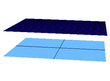
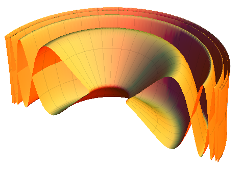
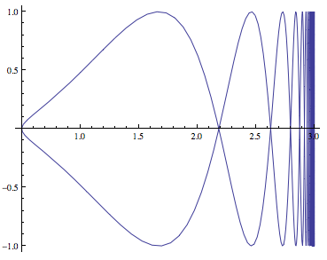
Example 9.2.

Consider the curve $\Gamma:\mathbb{R}\to\mathbb{R}^{3}$ parametrized as (see also figure 2):

$$\alpha_{R,a}(t)=\left(\frac{(R-a)t^{2}}{(t^{2}+1)}+a,0,\sin\left(\frac{(R-a)t^{3}}{(t^{2}+1)}+at\right)\right)$$

When it is rotated over the $(0,0,x_{3})$ axis, it generates a complete surface of revolution in $\mathbb{R}^{3}$ which is bounded, i.e. it can be kept inside a cylinder $\mathbb{R}\times\mathbb{S}^{1}$ with radius $R$ and height $h=1$. By using Theorem A this surface is recurrent. Note also that the mean curvature of this surface is unbounded.

Figure 2. A parabolic surface in a ball of $\mathbb{R}^{3}$ and its generating curve $\alpha_{R,a}(t)$.

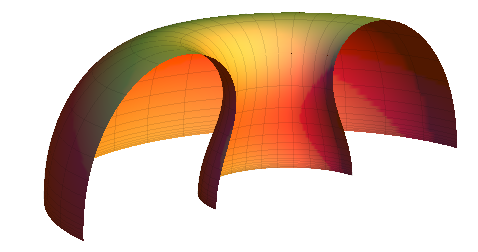
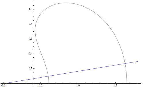
9.2. Surfaces in $\mathbb{H}^{3}$ with transcient Brownian movement

The spherical catenoids immersed in $\mathbb{H}^{3}$ are example of surfaces of revolution in $\mathbb{H}^{3}$ with transcient (non-recurrent) Brownian movement. Spherical catenoids have been studied in [dCD83], [Mor81] or [Seo11] and, specifically using the Upper Halfspace Model in [BSE10].

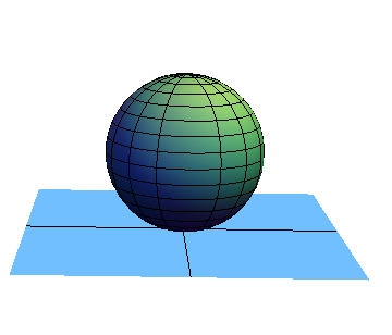
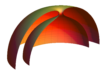
Example 9.3 (Spherical catenoids).

Spherical catenoids are the minimal complete surfaces of revolution generated by the rotation of the family of curves

$$\gamma_{a}(s)=\left(e^{\Lambda_{a}(s)}\tanh(y_{a}(s)),0,\frac{e^{\Lambda_{a}(s)}}{\cosh(y_{a}(s))}\right)$$

where

$$y_{a}(s):=a+\int_{0}^{s}\frac{\cosh(2a)\sinh(2t)}{(\cosh(2a)^{2}\cosh(2t)^{2}-1)^{\frac{1}{2}}}dt.$$

and

$$\Lambda_{a}(s):=\sqrt{2}\sinh(2a)\int_{0}^{s}\frac{(\cosh(2a)\cosh(2t)-1)^{\frac{1}{2}}}{\cosh^{2}(2a)\cosh^{2}(2t)-1}dt.$$

The warping function is thus given by

$$w_{-1}(s)=\frac{\gamma_{a1}(s)}{\gamma_{a2}(s)}=\sinh(y_{a}(s))$$

and hence the following integral can be showed as a divergent integral.

$$\int^{\infty}\frac{1}{w_{-1}(s)}ds=\int^{\infty}\frac{1}{\sinh(y_{a}(s))}ds<\infty$$

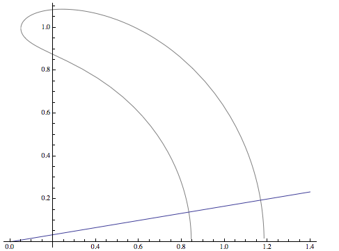
proving that each one of the ends of the surface is non-parabolic. However, transcience of spherical catenoids can be proved taking into account that spherical catenoids are minimal surfaces, and every minimal surface of $\mathbb{H}^{3}$ is transcient (see [MP03] for instance).

Observe (see figure 3) that by Theorem 4.1, the part of the curve $\gamma_{a}(s)$ lying over an arbitrary line $t\to(t,c\cdot t)$ has to be of finite length.

Figure 3. Half Spherical Catenoids immersed in $\mathbb{H}^{3}$: $\Sigma_{0.05}$ and $\Sigma_{0.5}$. Observe that the catenoid lies under a horosphere, the part of the profile curve lying over an arbitrary line $t\to(t,0,c\cdot t)$ has finite length (Theorem 4.1), each one of the two ends approaches to the plane $\{x_{3}=0\}$ (Corollary E), and $\sup x_{1}<\infty$ (Proposition 5.1).

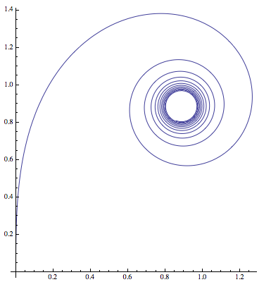
9.3. Surfaces in $\mathbb{H}^{3}$ with recurrent Brownian motion

To construct a surface of revolution in $\mathbb{H}^{3}$ with recurrent Brownian motion can be achieved, by using our Theorem B, if we construct a surface such that every end is of revolution and every end is on a $c$-cone for some $c>0$. In our example we are using clothoids.

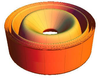
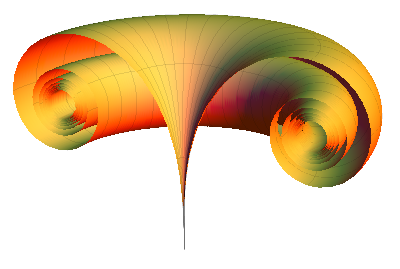
Example 9.4.

The clothoids or spirals of Cornu are curves generated by pairs of functions of the form

$$\text{clothoid}[n,a][t]=a\left(\int_{0}^{t}\sin\left(\frac{s^{n+1}}{n+1}\right)ds,0,\int_{0}^{t}\cos\left(\frac{s^{n+1}}{n+1}\right)ds\right)$$

and commonly used in construction (cf. [Gra98]). By changing $t\to e^{t}$, in case $a=n=1$, we obtain a complete curve which can be easily immersed in $\mathbb{H}^{2}$. The surface of revolution obtained when rotating the curve over the vertical axes appears to have two parabolic ends (see figure 4). Note that the immersion of the surface is not proper.

Figure 4. Clothoid or spiral of Cornu: the curve, the curve reparameterized, and the rotation with parameters $a=1,n=1$.

Example 9.5 (horosphere).

An other interesting example of surface of revolution is the horosphere which in the upper half space model of $\mathbb{H}^{3}$ is just the $x_{3}=z$ plane. An end of revolution can be obtained rotating the parametrized by arc length curve

$$\gamma:[0,\infty)\to\mathbb{H}^{3},\quad\gamma(s)=(z\,s+1,0,z)$$

along the $x_{3}$-axis. Observe that

$$w_{-1}(s)=\frac{\gamma_{1}(s)}{\gamma_{2}(s)}=s+\frac{1}{z}.$$

If we observe the movement of the centroid

$$x_{g}(\gamma([0,s])=\frac{\int_{0}^{s}w_{-1}(s)ds}{s}=\frac{s}{2}+\frac{1}{z}$$

Hence, given $s_{0}>0$, for any $s\geq s_{0}$ and denoting $C:=(\frac{1}{2}+\frac{1}{zs_{0}})$,

$$x_{g}(\gamma([0,s])=s(\frac{1}{2}+\frac{1}{zs})\leq C\,s$$

By Theorem 8.1 the horosphere is a recurrent surface. This result can be achieved directly by using Theorem C or by the fact that since the horosphere is a flat surface, it has finite total curvature and hence (by using [Ich82a]) the Brownian movement is recurrent.

9.4. Surfaces of revolution in $\mathbb{H}^{3}$ with one parabolic end and one non-parabolic end

The following example uses vertical lines instead of horizontal lines as in the horospheres

Example 9.6 (cylinders).

Figure 5. The cylinder immersed in $\mathbb{H}^{3}$ with parameters $b=2,c=1$. This surface has two ends, one parabolic and the other non-parabolic.

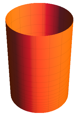
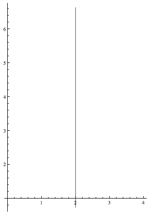
The family of parameterized curves in $\mathbb{H}^{3}$

$$\beta_{b,c}:(-\infty,\infty)\to\mathbb{H}^{3},\quad\beta_{b,c}(t)=(b,0,c\cdot e^{t})$$

can be rotated over the vertical axes $(0,x_{3})$ to get a cylinder (see figure 5). This surface of revolution in $\mathbb{H}^{3}$ has two ends of revolution in $\mathbb{H}^{3}$. One upper end $E^{+}$ given by the rotation of the parametrized by arc length curve

$$\gamma_{E^{+}}:[0,\infty)\to\mathbb{H}^{3},\quad\gamma_{b,c}(s)=(b,0,c\cdot e^{s})$$

And an other end $E^{-}$ obtained by the rotation of the parametrized by arc length curve

$$\gamma_{E^{-}}:[0,\infty)\to\mathbb{H}^{3},\quad\gamma_{b,c}(s)=(b,0,c\cdot e^{-s})$$

Observe that the end $E^{+}$ is on the $\frac{c}{b}$-cone, and hence by Theorem B is a parabolic end. On the other hand the end $E_{-}$ has

$$w_{-1}(s)=\frac{b}{c}e^{s}$$

thus

$$\int^{\infty}_{0}\frac{1}{w_{-1}(s)}ds=\int^{\infty}_{0}\frac{c}{b}e^{-s}ds=\frac{c}{b}<\infty$$

the end $E_{-}$ is therefore non-parabolic by using proposition 2.15.

References

- [Ahl35] Lars V. Ahlfors, Sur le type d’un surface de riemann, C.R. Acad. Sci. Paris 1 (1935), no. 201, 30–32.
- [Ahl52] by same author, On the characterization of hyperbolic Riemann surfaces, Ann. Acad. Sci. Fennicae. Ser. A. I. Math.-Phys. 1952 (1952), no. 125, 5. MR 0054729 (14,970a)
- [BdLPS13] G. Pacelli Bessa, Jorge H. de Lira, Stefano Pigola, and Alberto G. Setti, Curvature estimates for submanifolds immersed into horoballs and horocylinders, 2013.
- [BM07] G. Pacelli Bessa and J. Fábio Montenegro, An extension of Barta’s theorem and geometric applications, Ann. Global Anal. Geom. 31 (2007), no. 4, 345–362. MR 2325220 (2008e:53112)
- [BSE10] Pierre Bérard and Ricardo Sa Earp, Lindelöf’s theorem for hyperbolic catenoids, Proceedings of the American Mathematical Society 138 (2010), no. 10, 3657–3669.
- [dC92] Manfredo Perdigão do Carmo, Riemannian geometry, Mathematics: Theory & Applications, Birkhäuser Boston Inc., Boston, MA, 1992, Translated from the second Portuguese edition by Francis Flaherty. MR 1138207 (92i:53001)
- [dCD83] M. do Carmo and M. Dajczer, Rotation hypersurfaces in spaces of constant curvature, Trans. Amer. Math. Soc. 277 (1983), no. 2, 685–709. MR 694383 (85b:53055)
- [GH14] A. Grigor’yan and X. Huang, Stochastic completeness of jump processes on metric measure spaces, vol. 88, 2014, cited By 0, pp. 209–224.
- [Gim14] Vicent Gimeno, Isoperimetric inequalities for submanifolds. Jellett–Minkowski’s formula revisited, To appear in Proc. London Math. Soc. (2014), 1–22.
- [GMM00] José A. Gálvez, Antonio Martínez, and Francisco Milán, Flat surfaces in the hyperbolic -space, Math. Ann. 316 (2000), no. 3, 419–435. MR 1752778 (2002b:53013)
- [Gra98] Alfred Gray, Modern differential geometry of curves and surfaces with Mathematica, second ed., CRC Press, Boca Raton, FL, 1998. MR 1688379 (2000i:53001)
- [Gri99] Alexander Grigor′yan, Analytic and geometric background of recurrence and non-explosion of the Brownian motion on Riemannian manifolds, Bull. Amer. Math. Soc. (N.S.) 36 (1999), no. 2, 135–249. MR 1659871 (99k:58195)
- [Gri09] Alexander Grigor’yan, Heat kernel and analysis on manifolds, AMS/IP Studies in Advanced Mathematics, vol. 47, American Mathematical Society, Providence, RI, 2009. MR 2569498 (2011e:58041)
- [GW79] R. E. Greene and H. Wu, Function theory on manifolds which possess a pole, Lecture Notes in Mathematics, vol. 699, Springer, Berlin, 1979. MR 521983 (81a:53002)
- [Has60] R. Z. Has′minskiĭ, Ergodic properties of recurrent diffusion processes and stabilization of the solution of the Cauchy problem for parabolic equations, Teor. Verojatnost. i Primenen. 5 (1960), 196–214. MR 0133871 (24 #A3695)
- [HM90] D. Hoffman and W. H. Meeks, III, The strong halfspace theorem for minimal surfaces, Invent. Math. 101 (1990), no. 2, 373–377. MR 1062966 (92e:53010)
- [HP11] Ana Hurtado and Vicente Palmer, A note on the -parabolicity of submanifolds, Potential Anal. 34 (2011), no. 2, 101–118. MR 2754966 (2012e:53099)
- [Ich82a] Kanji Ichihara, Curvature, geodesics and the Brownian motion on a Riemannian manifold. I. Recurrence properties, Nagoya Math. J. 87 (1982), 101–114. MR 676589 (84m:58166a)
- [Ich82b] by same author, Curvature, geodesics and the Brownian motion on a Riemannian manifold. II. Explosion properties, Nagoya Math. J. 87 (1982), 115–125. MR 676590 (84m:58166b)
- [JX81] Luquésio P. de M. Jorge and Frederico V. Xavier, An inequality between the exterior diameter and the mean curvature of bounded immersions, Math. Z. 178 (1981), no. 1, 77–82. MR 627095 (82k:53080)
- [KN96] Shoshichi Kobayashi and Katsumi Nomizu, Foundations of differential geometry. Vol. I, Wiley Classics Library, John Wiley & Sons Inc., New York, 1996, Reprint of the 1963 original, A Wiley-Interscience Publication. MR 1393940 (97c:53001a)
- [Kob95] Shoshichi Kobayashi, Transformation groups in differential geometry, Classics in Mathematics, Springer-Verlag, Berlin, 1995, Reprint of the 1972 edition. MR 1336823 (96c:53040)
- [Lee97] John M. Lee, Riemannian manifolds, Graduate Texts in Mathematics, vol. 176, Springer-Verlag, New York, 1997, An introduction to curvature. MR 1468735 (98d:53001)
- [Lee03] by same author, Introduction to smooth manifolds, Graduate Texts in Mathematics, vol. 218, Springer-Verlag, New York, 2003. MR 1930091 (2003k:58001)
- [Li00] Peter Li, Curvature and function theory on Riemannian manifolds, Surveys in differential geometry, Surv. Differ. Geom., VII, Int. Press, Somerville, MA, 2000, pp. 375–432. MR 1919432 (2003g:53047)
- [Mor81] H. Mori, Minimal surfaces of revolution in and their global stability, Indiana Univ. Math. Jour. 30 (1981), 787–794.
- [MP03] S. Markvorsen and V. Palmer, Transience and capacity of minimal submanifolds, Geom. Funct. Anal. 13 (2003), no. 4, 915–933. MR 2006562 (2005d:58064)
- [MP04] William H. Meeks, III and Joaquín Pérez, Conformal properties in classical minimal surface theory, Surveys in differential geometry. Vol. IX, Surv. Differ. Geom., IX, Int. Press, Somerville, MA, 2004, pp. 275–335. MR 2195411 (2006k:53015)
- [MP10] Steen Markvorsen and Vicente Palmer, Extrinsic isoperimetric analysis of submanifolds with curvatures bounded from below, J. Geom. Anal. 20 (2010), no. 2, 388–421. MR 2579515 (2011c:53131)
- [Nad96] Nikolai Nadirashvili, Hadamard’s and Calabi-Yau’s conjectures on negatively curved and minimal surfaces, Invent. Math. 126 (1996), no. 3, 457–465. MR 1419004 (98d:53014)
- [Nev40] Rolf Nevanlinna, Ein Satz über offene Riemannsche Flächen, Ann. Acad. Sci. Fennicae (A) 54 (1940), no. 3, 18. MR 0003813 (2,276c)
- [Pet98] Peter Petersen, Riemannian geometry, Graduate Texts in Mathematics, vol. 171, Springer-Verlag, New York, 1998. MR 1480173 (98m:53001)
- [RR98] Lucio Rodriguez and Harold Rosenberg, Half-space theorems for mean curvature one surfaces in hyperbolic space, Proc. Amer. Math. Soc. 126 (1998), no. 9, 2755–2762. MR 1458259 (98k:53015)
- [Seo11] Keomkyo Seo, Stable minimal hypersurfaces in the hyperbolic space, J. Korean Math. Soc. 48 (2011), no. 2, 253–266. MR 2789454 (2012c:53096)
- [Tro99] M. Troyanov, Parabolicity of manifolds, Siberian Adv. Math. 9 (1999), no. 4, 125–150. MR 1749853 (2001e:31013)