The clustering of radio galaxies: biasing and evolution versus stellar mass

Abstract

We study the angular clustering of $\sim 6\times 10^{5}$ NVSS sources on scales $\lower 2.15277pt\hbox{$\;\buildrel>\over{\sim}\;$}50h^{-1}\,{\rm Mpc}$ in the context of the $\Lambda$CDM scenario. The analysis partially relies on the redshift distribution of 131 radio galaxies, inferred from the Hercules and CENSORS survey, and an empirical fit to the stellar to halo mass (SHM) relation. For redshifts $z\lower 2.15277pt\hbox{$\;\buildrel<\over{\sim}\;$}0.7$, the fraction of radio activity versus stellar mass evolves as $f_{{}_{\rm RL}}\sim M_{*}^{\alpha_{0}+\alpha_{1}z}$ where $\alpha_{0}=2.529{\pm 0.184}$ and $\alpha_{1}=1.854^{+0.708}_{-0.761}$. The estimate on $\alpha_{0}$ is largely driven by the results of Best et al. (2005), while the constraint on $\alpha_{1}$ is new. We derive a biasing factor $b(z=0.5)=2.093^{+0.164}_{-0.109}$ between radio galaxies and the underlying mass. The function $b(z)=0.33z^{2}+0.85z+1.6$ fits well the redshift dependence. We also provide convenient parametric forms for the redshift dependent radio luminosity function, which are consistent with the redshift distribution and the NVSS source count versus flux.

1. Introduction

Radio activity is a marker for energetic processes related to star formation and accretion of gas on super massive black holes (SMBHs) at the nuclei of galaxies. Active Galactic Nuclei (AGN) are associated with cycles of powerful jets generated by accretion disks on SMBH. These jets make a sizable contribution to the energy budget at moderate redshifts and can play an important role in galaxy formation (e.g. Binney & Tabor, 1995; Bower et al., 2006; Croton et al., 2006) and even offsetting gas cooling in massive groups and clusters of galaxies (e.g. Boehringer et al., 1993; Carilli et al., 1994; McNamara et al., 2000). Therefore, the interplay between radio activity and other galaxy characteristics is of great interest (e.g Best et al., 2005; Fontanot et al., 2011). The environment, whether galaxies are isolated or in dense regions, may also have an important impact on the emergence of radio activity. Galaxy-galaxy interactions tend to boost accretion of gas on the central SMBH (e.g. Best et al., 2005; Pasquali et al., 2009), eventually triggering AGN activity. One approach is to directly assess the observed galaxy environment of radio AGNs (e.g. Prestage & Peacock, 1988; Hill & Lilly, 1991; McLure & Dunlop, 2001; Best et al., 2005; Worpel et al., 2013), but this is typically limited by small sample uncertainties. Alternatively, the clustering of radio galaxies quantified through two-point statistics (e.g. correlation functions), could constrain the way these galaxies are related to the underlying mass density field and and the properties of the host dark halos (e.g. Peacock & Nicholson, 1991; Lacy, 2000; Passmoor et al., 2013; Blake et al., 2004). Unfortunately, redshift surveys of radio galaxies contain a small number of objects(Mauch & Sadler, 2007; Brown et al., 2011; Donoso et al., 2010; van Velzen et al., 2012) and are currently unsuitable for a robust determination of two point statistics at moderate redshifts. Here we revisit the angular power spectrum computed from radio sources in the NRAO VLA Sky Survey (NVSS) (Condon et al., 1998). The survey provides angular positions and 1.4GHz fluxes, $S$, for about 80% of the sky and is currently the most suitable survey for angular angular clustering analysis.

Two ingredients are needed for extracting information from angular clustering statistics within a cosmological scenario, e.g. the $\Lambda$CDM. The first is a model for the mean redshift distribution, $N(z)$, of NVSS sources (galaxies). We base our modeling of $N(z)$ on two catalogs of radio sources with redshifts but small angular coverage. These are the Combined EIS-NVSS Survey (CENSORS)(Best et al., 2003; Rigby et al., 2011) and the Hercules survey (Waddington et al., 2001) which are (jointly) complete down to a flux limit of $7.2\rm mJy$. The second ingredient is the biasing relation between the spatial distribution of radio galaxies and the underlying mass density field. Our modeling of this relation adopts a parametric form for the frequency of radio activity versus stellar mass and an observationally motivated stellar to halo mass (SHM) ratio from the literature. Well established halo biasing is then incorporated to yield a prescription for the biasing relation of radio galaxies. The angular power spectrum of radio galaxies as predicted in the $\Lambda$CDM is then contrasted with the clustering of NVSS galaxies in order to put constraints the biasing relation and the prevalence of radio activity as a function of the stellar mass and redshift.

The outline of the paper is as follows. In §2 we review the definition of the angular power spectrum, $C_{l}$, and how it is estimated from the data with partial sky coverage. The calculation of the theoretical $C_{l}$ in the context of a cosmological model is presented in §2.2. This section also describes our modeling of the biasing relation and the redshift distribution of radio galaxies. In §3 we give the maximum likelihood methodology for parameter estimation. Constraints on the biasing and the evolution of radio activity are derived in §4. In §5, our model for the redshift distribution is shown to be consistent with observations of the radio luminosity function and the source counts in the NVSS. We end in §6 with a general discussion of the results.

2. The angular power spectrum

We define the surface number density contrast of sources

$$\Delta(\hat{\kern-0.24994pt\hbox{$r$}\kern-4.78937pt\kern 0.50003pt\hbox{$r$}\kern-4.78937pt\kern-0.24994pt\raise 0.43304pt\hbox{$r$}})=\frac{{\cal N}(\hat{\kern-0.24994pt\hbox{$r$}\kern-4.78937pt\kern 0.50003pt\hbox{$r$}\kern-4.78937pt\kern-0.24994pt\raise 0.43304pt\hbox{$r$}})}{\bar{\cal N}}-1\;,$$ (1)

where ${\cal N}(\hat{\kern-0.24994pt\hbox{$r$}\kern-4.78937pt\kern 0.50003pt\hbox{$r$}\kern-4.78937pt\kern-0.24994pt\raise 0.43304pt\hbox{$r$}})$ is the projected number density (per steradian) in the direction $\hat{\kern-0.24994pt\hbox{$r$}\kern-4.78937pt\kern 0.50003pt\hbox{$r$}\kern-4.78937pt\kern-0.24994pt\raise 0.43304pt\hbox{$r$}}$ and $\bar{\cal N}$ is the mean of ${\cal N}$ over the sky. In practice ${\cal N}(\hat{\kern-0.24994pt\hbox{$r$}\kern-4.78937pt\kern 0.50003pt\hbox{$r$}\kern-4.78937pt\kern-0.24994pt\raise 0.43304pt\hbox{$r$}})$ is obtained by dividing the sky into small pixels (e.g. via HEALPix (Gorski et al., 2005)) and counting the number of sources in each pixel. We decompose $\Delta(\hat{\kern-0.24994pt\hbox{$r$}\kern-4.78937pt\kern 0.50003pt\hbox{$r$}\kern-4.78937pt\kern-0.24994pt\raise 0.43304pt\hbox{$r$}})$ in spherical harmonics $Y_{lm}$ as

$${d_{lm}}=\int_{\rm survey}d\Omega\Delta(\hat{\kern-0.24994pt\hbox{$r$}\kern-4.78937pt\kern 0.50003pt\hbox{$r$}\kern-4.78937pt\kern-0.24994pt\raise 0.43304pt\hbox{$r$}})Y_{lm}(\hat{\kern-0.24994pt\hbox{$r$}\kern-4.78937pt\kern 0.50003pt\hbox{$r$}\kern-4.78937pt\kern-0.24994pt\raise 0.43304pt\hbox{$r$}})\;.$$ (2)

We imagine now that ${d_{lm}}$ is one out of an ensemble of many realizations of the same underlying continuous field. The variance, $<|{d_{lm}}|^{2}>_{{}_{\rm ens}}$, from this ensemble is approximated as (Peebles, 1980),

$$<|{d_{lm}}|^{2}>_{{}_{\rm ens}}=\left(C_{l}+\frac{1}{\bar{\cal N}}\right)J_{lm}\;,$$ (3)

where the term involving $\bar{\cal N}$ (mean number density over the observed part of the sky) appears due to the Poisson discrete sampling (shot-noise) of the continuous field by a finite number of sources and

$$J_{lm}=\int_{{}_{\rm survey}}|Y_{lm}|^{2}{\rm d}\Omega\;,$$ (4)

accounts for the partial sky coverage and gives unity for full sky data. The quantity $C_{l}$ is the underlying angular power spectrum in the continuous limit ($\bar{\cal N}\rightarrow\infty$) for full sky coverage. It is independent of $m$ by the assumption of cosmological isotropy, i.e. the lack of a preferred direction. According to (3), an estimate of the true power spectrum from the observations is

$$C^{\rm obs}_{l}=\frac{1}{2l+1}\sum_{m}\frac{|{d_{lm}}|^{2}}{J_{lm}}-\frac{1}{\bar{\cal N}}\;.$$ (5)

The $1\sigma$ error in this estimate is (Peebles, 1980, cf. §3 here)

$$\sigma_{{}_{{C_{l}}}}=\sqrt{\frac{2}{2l+1}}\left({C_{l}}^{\rm obs}+\frac{1}{\bar{\cal N}}\right)\;$$ (6)

reflecting cosmic variance and shot-noise scatter.

2.1. The measured $C_{l}$

The NVSS contains $\sim$1.7 billion sources with angular positions at 1.4 GHz integrated flux density $S>2.5\rm mJy$. The full width at half maximum resolution is 45 arcsec and nearly all observations are at uniform sensitivity. The catalogue covers the sky north of declination $-40^{\circ}$ (J2000) which is almost 80$\%$ of the celestial sphere. We trim the data as follows (Blake & Wall, 2002).

• Galactic sources at latitudes $|b|<5^{\circ}$ are masked out to avoid Galactic contamination.

• We remove 22 bright extended local radio galaxies.

• As shown by Blake & Wall (2002), the NVSS has significant systematic gradients in surface density for sources fainter than $10~{}\rm mJy$. Therefore, the analysis is restricted to sources brighter than 10 mJy. We also discard extra bright sources ($S>1000~{}\rm mJy$).

This leaves us with 574466 sources which we use here to derive the observed angular power spectrum, $C^{\rm obs}_{l}$, according to (5). The effect of multiple-component sources (e.g. radio lobes of the same galaxies) have been removed following the recipe of Blake et al. (2004). The blue filled dots in figure 1 are $C^{\rm obs}_{l}$ for all values of $l$ between $l>l_{\rm min}=4$ and $l<l_{\rm max}=100$ corresponding to comoving physical scales of $\lower 2.15277pt\hbox{$\;\buildrel>\over{\sim}\;$}50\rm h^{-1}\,{\rm Mpc}$ at $z=0.5$. The partial sky coverage introduces mixing of power between different $l$-modes. We have assessed this mixing in random realizations of the surface density $\Delta$, generated from the $\Lambda$CDM cosmological model (see below) and found it to be negligible for $l>3$. Hence, we impose a lower cut at $l=l_{\rm min}=4$. Since we shall restrict the analysis to large scales, we also impose a high $l$ threshold at $l=l_{\rm max}=100$. In practice, for $l>l_{\rm max}=100$, the signal to noise ratio becomes very small such that no significant information is lost by the restriction to $l<l_{lmax}$. We have confirmed that $C^{\rm obs}_{l}$ in this figure agrees very well with Blake et al. (2004).

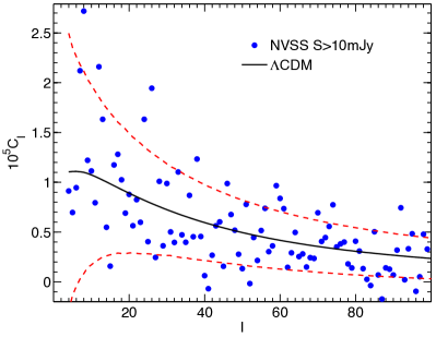
Figure 1.— The observed angular power spectrum estimated from the NVSS data for $S>10\rm mJy$ is shown as the blue dots. The solid curve is the $\Lambda$CDM ${\tilde{C}}_{l}$ obtained using the ML parameters given in Table 1. The dashed red curves correspond to $1\sigma$ limits due to shot-noise and cosmic variance scatter.

2.2. Theoretical $C_{l}$

We derive here theoretical expressions for angular power spectra of $\Delta(\hat{\kern-0.24994pt\hbox{$r$}\kern-4.78937pt\kern 0.50003pt\hbox{$r$}\kern-4.78937pt\kern-0.24994pt\raise 0.43304pt\hbox{$r$}})$ within a cosmological scenario. The redshift is denoted by $z$ and the comoving coordinate by $r$$r$$r$. By $z(r)$ we mean the redshift of a particle at a comoving distance $r$ in a uniform cosmological background. The underlying mass density field is $\rho^{\rm m}(\kern-0.24994pt\hbox{$r$}\kern-4.78937pt\kern 0.50003pt\hbox{$r$}\kern-4.78937pt\kern-0.24994pt\raise 0.43304pt\hbox{$r$},z)$ and the corresponding density contrast is $\delta^{\rm m}(\kern-0.24994pt\hbox{$r$}\kern-4.78937pt\kern 0.50003pt\hbox{$r$}\kern-4.78937pt\kern-0.24994pt\raise 0.43304pt\hbox{$r$},z)=\rho^{\rm m}(\kern-0.24994pt\hbox{$r$}\kern-4.78937pt\kern 0.50003pt\hbox{$r$}\kern-4.78937pt\kern-0.24994pt\raise 0.43304pt\hbox{$r$},z)/\bar{\rho}^{\rm m}-1$ where $\bar{\rho}^{\rm m}$ is the mean background density. The density contrast of galaxies is denoted by $\delta$.

The theoretical counterpart of $\Delta(\hat{\kern-0.24994pt\hbox{$r$}\kern-4.78937pt\kern 0.50003pt\hbox{$r$}\kern-4.78937pt\kern-0.24994pt\raise 0.43304pt\hbox{$r$}})$ is

$$\tilde{\Delta}(\hat{\kern-0.24994pt\hbox{$r$}\kern-4.78937pt\kern 0.50003pt\hbox{$r$}\kern-4.78937pt\kern-0.24994pt\raise 0.43304pt\hbox{$r$}})=\int_{0}^{\infty}\delta(\hat{\kern-0.24994pt\hbox{$r$}\kern-4.78937pt\kern 0.50003pt\hbox{$r$}\kern-4.78937pt\kern-0.24994pt\raise 0.43304pt\hbox{$r$}}r,z(r))p(r){\rm d}r\;,$$ (7)

where $\delta$ is the density contrast in the three dimensional distribution of galaxies at a comoving coordinate $r$$r$$r$ redshift $z=z(r)$. The quantity $p(r){\rm d}r$ is the probability of observing a galaxy between $r$ and $(r+{\rm d}r)$.

The cosmological model provides the statistical properties of the underlying mass density contrast field $\delta^{\rm m}(\kern-0.24994pt\hbox{$r$}\kern-4.78937pt\kern 0.50003pt\hbox{$r$}\kern-4.78937pt\kern-0.24994pt\raise 0.43304pt\hbox{$r$},z)$, rather than the galaxy density contrast $\delta$. Restricting the analysis to large scales (larger than a few 10s of Mpc) we assume here a linear biasing relation $\delta(\kern-0.24994pt\hbox{$r$}\kern-4.78937pt\kern 0.50003pt\hbox{$r$}\kern-4.78937pt\kern-0.24994pt\raise 0.43304pt\hbox{$r$},z)=b(z)\delta^{m}(\kern-0.24994pt\hbox{$r$}\kern-4.78937pt\kern 0.50003pt\hbox{$r$}\kern-4.78937pt\kern-0.24994pt\raise 0.43304pt\hbox{$r$},z)$, as motivated by the measured three dimensional correlation function of galaxies in redshift surveys (e.g. Norberg et al., 2001; Zehavi et al., 2011; Davis et al., 2011) and analytic studies of galaxy formation (Nusser et al., 2014). Further, on large scales, linear gravitational instability paradigm yields $\delta^{\rm m}(\kern-0.24994pt\hbox{$r$}\kern-4.78937pt\kern 0.50003pt\hbox{$r$}\kern-4.78937pt\kern-0.24994pt\raise 0.43304pt\hbox{$r$},z)=\delta^{m}_{0}(\kern-0.24994pt\hbox{$r$}\kern-4.78937pt\kern 0.50003pt\hbox{$r$}\kern-4.78937pt\kern-0.24994pt\raise 0.43304pt\hbox{$r$})D(z)$ where $D$ is the linear growth factor of linear fluctuations normalized to unity at the present time, $z=0$ (Peebles, 1980). Therefore,

$${{\tilde{a}}_{lm}} = \int d\Omega\tilde{\Delta}Y_{lm}(\hat{\kern-0.24994pt\hbox{$r$}\kern-4.78937pt\kern 0.50003pt\hbox{$r$}\kern-4.78937pt\kern-0.24994pt\raise 0.43304pt\hbox{$r$}})$$

$$= \int d\Omega Y_{lm}(\hat{\kern-0.24994pt\hbox{$r$}\kern-4.78937pt\kern 0.50003pt\hbox{$r$}\kern-4.78937pt\kern-0.24994pt\raise 0.43304pt\hbox{$r$}})\int_{0}^{\infty}W(r)\delta_{0}(\hat{\kern-0.24994pt\hbox{$r$}\kern-4.78937pt\kern 0.50003pt\hbox{$r$}\kern-4.78937pt\kern-0.24994pt\raise 0.43304pt\hbox{$r$}}r)dr\;,$$

where $W=D(z)b(z)p(r)$ with $z=z(r)$. Going to the Fourier domain

$$\delta_{0}(\kern-0.24994pt\hbox{$r$}\kern-4.78937pt\kern 0.50003pt\hbox{$r$}\kern-4.78937pt\kern-0.24994pt\raise 0.43304pt\hbox{$r$})=\frac{1}{(2\pi)^{3}}\int d^{3}k\delta_{\kern-0.17496pt\hbox{$k$}\kern-3.86458pt\kern 0.35002pt\hbox{$k$}\kern-3.86458pt\kern-0.17496pt\raise 0.30313pt\hbox{$k$}}{\rm e}^{i\kern-0.17496pt\hbox{$k$}\kern-3.86458pt\kern 0.35002pt\hbox{$k$}\kern-3.86458pt\kern-0.17496pt\raise 0.30313pt\hbox{$k$}\cdot{\kern-0.17496pt\hbox{$r$}\kern-3.35255pt\kern 0.35002pt\hbox{$r$}\kern-3.35255pt\kern-0.17496pt\raise 0.30313pt\hbox{$r$}}}\;,$$ (9)

and substituting ${\rm e}^{i\kern-0.17496pt\hbox{$k$}\kern-3.86458pt\kern 0.35002pt\hbox{$k$}\kern-3.86458pt\kern-0.17496pt\raise 0.30313pt\hbox{$k$}\cdot{\kern-0.17496pt\hbox{$r$}\kern-3.35255pt\kern 0.35002pt\hbox{$r$}\kern-3.35255pt\kern-0.17496pt\raise 0.30313pt\hbox{$r$}}}=4\pi\sum_{l}{\rm i}^{l}j_{l}(kr)Y^{*}_{lm}(\hat{\kern-0.24994pt\hbox{$n$}\kern-6.00235pt\kern 0.50003pt\hbox{$n$}\kern-6.00235pt\kern-0.24994pt\raise 0.43304pt\hbox{$n$}})Y_{lm}(\hat{\kern-0.24994pt\hbox{$k$}\kern-5.52084pt\kern 0.50003pt\hbox{$k$}\kern-5.52084pt\kern-0.24994pt\raise 0.43304pt\hbox{$k$}})$, yields,

$${{\tilde{a}}_{lm}}=\frac{{\rm i}^{l}}{2\pi^{2}}\int drW\int d^{3}k\delta_{\kern-0.17496pt\hbox{$k$}\kern-3.86458pt\kern 0.35002pt\hbox{$k$}\kern-3.86458pt\kern-0.17496pt\raise 0.30313pt\hbox{$k$}}j_{l}(kr)Y^{*}_{lm}(\hat{\kern-0.24994pt\hbox{$k$}\kern-5.52084pt\kern 0.50003pt\hbox{$k$}\kern-5.52084pt\kern-0.24994pt\raise 0.43304pt\hbox{$k$}})\;.$$ (10)

Therefore,

$${\tilde{C}}_{l} = <|{{\tilde{a}}_{lm}}|^{2}>$$

$$= \frac{2}{\pi}\int dkk^{2}P(k)\left|\int_{0}^{\infty}drWj_{l}(kr)\right|^{2}\;.$$

and we have used $<\delta_{\kern-0.17496pt\hbox{$k$}\kern-3.86458pt\kern 0.35002pt\hbox{$k$}\kern-3.86458pt\kern-0.17496pt\raise 0.30313pt\hbox{$k$}}\delta_{\kern-0.17496pt\hbox{$k$}\kern-3.86458pt\kern 0.35002pt\hbox{$k$}\kern-3.86458pt\kern-0.17496pt\raise 0.30313pt\hbox{$k$}^{\prime}}>=(2\pi)^{3}\delta^{\rm D}(\kern-0.24994pt\hbox{$k$}\kern-5.52084pt\kern 0.50003pt\hbox{$k$}\kern-5.52084pt\kern-0.24994pt\raise 0.43304pt\hbox{$k$}-\kern-0.24994pt\hbox{$k$}\kern-5.52084pt\kern 0.50003pt\hbox{$k$}\kern-5.52084pt\kern-0.24994pt\raise 0.43304pt\hbox{$k$}^{\prime})P(k)$ where $\delta^{\rm D}$ is Dirac’s $\delta-$function. The power spectrum $P(k)$ of linear density fluctuations is well constrained by a variety of observations, primarily the cosmic microwave anisotropies measured by the Planck satellite (Planck Collaboration et al., 2015). The remaining ingredients in the theoretical modeling are the radial distribution $p(r)$ and the biasing $b(z)$.

2.2.1 The radial distribution

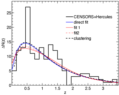
Figure 2.— The histogram is the observed number of sources with $S>7.2~{}\rm mJy$ per redshift bin $\Delta z=0.15$. The curves “fit 1” & “fit 2” are obtained using two parametric forms for the radio luminosity function as described in §5.

The modeling of $p(r)$ relies on CENSORS )(Best et al., 2003; Rigby et al., 2011) and Hercules (Waddington et al., 2001) surveys of radio galaxies with observed redshifts and 1.4GHz fluxes. CENSORS contains 135 radio sources over $\rm 6deg^{2}$ complete down to $7.2\;\rm mJy$ 1.4GHz flux limit. Spectroscopic redshifts are available for about $73\%$ of the sources. The remaining sources have been assigned redshifts through the $I-z$ or $K-z$ magnitude-redshift relations. In Hercules, there are 64 objects 1.2 $\rm deg^{2}$ with $S>2\;\rm mJy$. The two surveys together contain 165 and 131 sources, respectively for $S>\;\rm 7.2mJy$ and $10\;\rm mJy$.

The number of sources per unit redshift, $N(z)$, in the two surveys jointly is the basis for our model of $p(r)\propto N(z){\rm d}z/{\rm d}r$. The distribution $N(z)$ is represented by the histogram in figure 2. According to Rigby et al. (2011), there is a difficulty in obtaining spectroscopic redshifts at $z\approx 1.5$, resulting in the observed gap in $N(z)$. Less accurate redshift measurements compensate but the random error scatter objects to the sides. As we shall see at a later stage, the angular clustering probes large scale structure $\lower 2.15277pt\hbox{$\;\buildrel<\over{\sim}\;$}0.7$. Hence, the results are insensitive to whether galaxies near the gap are included or not in the modeling of $p(r)$. Since the number of galaxies is too small for a robust measurement of $N(z)$, we adopt the parametric form for $N(z)\propto p(r){\rm d}r/{\rm d}z$,

$$N^{\rm model}\propto z^{a_{1}}\exp\left[-\left(\frac{z}{a_{2}}\right)^{a_{3}}\right]\;,$$ (12)

where the parameters $a_{1}$, $a_{2}$ and $a_{3}$ are determined by maximizing the probability distribution for measuring $N(z)$ as well as the observed angular power spectrum, $C_{l}$. Further, we impose a upper redshift cutoff in the abundance of sources at $z=3.5$, consistent with decline in their number density as seen by Rigby et al. (2011). In this modeling we use the redshift distribution of galaxies with $S>10\rm mJy$ to match the flux limit of the trimmed version of the NVSS, as described in §2.1. The normalization of $N^{\rm model}$ is such that it yields the total number of sources ($S>10\rm mJy$) in the joint CENSORS and Hercules data. For a Poisson distribution of $N$, this is equivalent to performing a maginalization over the normalization.

2.2.2 The biasing relation

We will resort to a variety of observational results to link radio galaxies to the masses of their host dark matter halos. A description for the biasing of radio galaxies will then be obtained from well-established relations between the halo distribution and the mass density field.

Best et al. (2005) studied the properties of the host galaxies of a local ($z<0.1$) sample of radio-loud AGN. They demonstrated: $i)$ the presence of radio activity is a strong function, $M_{*}^{2.5}$, of the stellar mass, $M_{*}$, of the host galaxies, saturating at $\sim 30\%$ for $M_{*}\lower 2.15277pt\hbox{$\;\buildrel>\over{\sim}\;$}10^{12}M_{\odot}$. $ii)$ the shape of the radio luminosity distribution in galaxies with a similar stellar mass, $M_{*}$, depends very weakly on $M_{*}$ and is close to the global luminosity function (Mauch & Sadler, 2007; Best et al., 2014). We assume that similar trends extend to higher redshifts and write the fraction of radio loud AGNs with radio luminosity brighter than $P$ as

$$f_{{}_{\rm RL}}={\cal F}(M_{*},z)\Phi(P,z)\;,$$ (13)

where $\Phi(P,0)$ is close to the global radio luminosity. Further, we adopt

$${\cal F}(M_{*},z)=\left(\frac{M_{*}}{10^{11}M_{\odot}}\right)^{\alpha_{0}+\alpha_{1}z}\;,$$ (14)

where $\alpha_{0}=2.5\pm 0.2$ (Best et al., 2005) will be included as a prior in the maximum likelihood analysis presented below. The fraction of radio activity is practically nonexistence at $M_{*}<10^{10}M_{\odot}$ (Best et al., 2005). One of the main goals of this paper is to constrain $\alpha_{1}$ from the clustering of the NVSS galaxies and the inferred $N(z)$ from the CENSORS and Hercules. Since the stellar and halo masses are closely related, the dependence of radio activity on $M_{*}$ dictates the biasing of the radio galaxies through the well studied halo biasing. We assume that the radio luminosity depends on the halo mass, $M$, only through $M_{*}$ hence the form of $\tilde{\Phi}(P,z)$ is irrelevant for the biasing prescription. We further assume that there is only radio galaxy per halo. This is incorrect for low luminosities as seen in galaxy clusters (Branchesi et al., 2005), but it is a reasonable assumption for the luminosities considered here. Therefore, we write the biasing factor as

$$b(z)=\frac{\int_{M_{\rm min}}^{M_{\rm max}}{\rm d}Mn_{\rm h}(M,z)b_{\rm h}(M,z){\cal F}(M_{*},z)}{\int_{M_{\rm d}}^{M_{\rm u}}{\rm d}Mn_{\rm h}(M,z){\cal F}(M_{*},z)}\;,$$ (15)

where the stellar mass $M_{*}$ as a function of the halo mass, $M$, and redshift is taken from the SHM relation derived by (Moster et al., 2013). This relation is in reasonable agreement with a variety of observations at low and high redshifts (c.f. Coupon et al., 2015). The mass thresholds $M_{\rm min}$ and $M_{\rm max}$ are, respectively, the minimum and maximum halo masses that can host a radio galaxy. We take $M_{\rm min}=4\times 10^{11}M_{\odot}$, corresponding to $M_{*}=10^{10}M_{\odot}$ (Moster et al., 2013) which is the lowest stellar mass exhibiting radio activity. As we will see later, because of the steep dependence of ${\cal F}$ on $M_{*}$, the results are insensitive to the exact value of $M_{\rm min}$. At the high mass end we take $M_{\rm max}=10^{15}M_{\odot}$, the mass scale of rich galaxy clusters. Halos with this large mass are rare, implying that our analysis in insensitive to this upper bound as well.

3. Likelihood analysis

Within the context of the $\Lambda$CDM cosmology, we seek constraints on the 5 parameters $\alpha_{0}$, $\alpha_{1}$, $a_{1}$, $a_{2}$ and $a_{2}$ by maximizing the likelihood, $P_{\rm tot}$, for observing ${C_{l}}^{\rm d}$ (from NVSS) and $N(z)$ (from the joint CENSORS and Hercules catalogs). For brevity, we denote these parameters by $\theta_{i}$ ($i=1\cdots 5$). We derive now the expression for $P_{\rm tot}$. Let $\tilde{d}_{lm}=d_{lm}/J^{1/2}_{lm}$ and continue to assume that the partial sky coverage does not introduce significant statistical correlation between $\tilde{d}_{lm}$ with different $(l,m)$. Restricting the analysis to large scales, the probability distribution function (PDF) of $\tilde{d}_{lm}$ is gaussian

$$P(\tilde{d}_{lm})\propto\frac{1}{({C_{l}}+1/\bar{\cal N})^{1/2}}{\exp}\left[-\frac{1}{2}\frac{\tilde{d}_{lm}^{2}}{{C_{l}}+1/{\bar{\cal N}}}\right]\;,$$ (16)

where $<\tilde{d}_{lm}^{2}>={C_{l}}+1/\bar{\cal N}$ in accordance with (3). The PDF of the full set $\{\tilde{d}_{lm}\}$ of all $m=-l\cdots+l$ is

$$P_{l}\propto\frac{1}{({C_{l}}+1/\bar{\cal N})^{l+1/2}}{\exp}\left(-\frac{2l+1}{2}\frac{{C_{l}}^{\rm d}}{{C_{l}}+1/\bar{\cal N}}\right)\;,$$ (17)

where ${C_{l}}^{\rm d}=(\sum_{m}d_{lm}^{2})/(2l+1)$. Maximizing $P_{l}$ with respect to ${C_{l}}$ yields ${C_{l}}={C_{l}}^{\rm d}-{\bar{\cal N}}^{-1}=C^{\rm obs}_{l}$ (c.f. eq. 3) as expected. An estimate of the $1\sigma$ error on this ${C_{l}}$ is $\sigma_{{}_{{C_{l}}}}=(-{\rm d}^{2}{\rm ln}P/{\rm d}{C_{l}}^{2})^{-1/2}=({C_{l}}+{\bar{\cal N}}^{-1})\sqrt{2/(2l+1)}$ (cf. Eq. 6). We write the likelihood function for observing ${C_{l}}^{d}$ and $N(z)$ as

$$P_{\rm tot}(\{\theta_{i}\};N,{C_{l}}^{\rm d})=P_{\alpha_{0}}\prod_{z_{i}}P_{{}_{\rm{N_{i}}}}\prod_{l=l_{\rm min}}^{l_{\rm max}}P_{l}\;,$$ (18)

where $P_{\alpha_{0}}$ a (Gaussian) prior PDF incorporating the local, $z\approx 0$, observational constraint $\alpha_{0}=2.5\pm 0.2$ of Best et al. (2005). Further, $P_{{}_{\rm{N_{i}}}}$ is a Poisson PDF for observing $N_{i}$ galaxies in the redshift bin $i$ given a mean number of $N^{\rm model}(z_{i})\Delta z$. We will use the redshift distribution of sources with $S>10\rm mJy$ and $\Delta z=0.15$. The probability $P_{l}$ is given by (17) with ${C_{l}}=\tilde{C}_{l}$ computed using the Eisenstein & Hu (1998) parametrized form of the $\Lambda$CDM density power spectrum, $P(k)$. The cosmological parameters are taken from the latest Planck results (Planck Collaboration et al., 2015): Hubble constant $H_{0}=67.8\rm kms^{-1}Mpc^{-1}$, total matter density parameter $\Omega_{m}=0.308$, baryonic density parameter $\Omega_{b}=0.0486$, linear clustering amplitude on $8h^{-1}\,{\rm Mpc}$ scale, $\sigma_{8}=0.815$ and a spectral index $n_{s}=0.9667$.

The evaluation of ${\tilde{C}}_{l}$ with full direct numerical integration is very slow. Fortunately, the Limber approximation is accurate to better than 5% even at small $l$, as revealed by comparison with the full calculation for some relevant choices of the parameters. Substitution of the Limber approximation

$$\int drW(r)j_{l}(kr)\approx\sqrt{\frac{\pi}{2l+1}}k^{-1}W\left(r=\frac{l+1/2}{k}\right)$$ (19)

in (2.2) yields,

$${\tilde{C}}_{l} = \frac{2}{2l+1)}\int_{0}^{\infty}dkP(k)W^{2}\left(r=\frac{l+1/2}{k}\right)$$ (20)

$$= \int_{0}^{\infty}drr^{-2}P\left(\frac{l+1/2}{r}\right)W^{2}(r)\;.$$

4. Results

We fix $l_{\rm min}=4$ and $l_{\rm max}=100$, as the fiducial values. Table 1 lists the parameters $\theta_{i}=\theta^{\rm ML}_{i}$ obtained by maximizing $P_{\rm tot}$. The theoretical ${\tilde{C}}_{l}$ computed with these parameters, is shown in figure 1 as the black solid curve. The dashed red lines are $1\sigma$ deviations from ${\tilde{C}}_{l}$ due to the combined error of shot-noise and cosmic variance, i.e., $\pm({\tilde{C}}_{l}+1/\bar{\cal N})\sqrt{2/(2l+1)}$. The scatter of the blue points around ${\tilde{C}}_{l}$ is entirely consistent with this error, as confirmed using random samples of $d_{lm}$ generated assuming ${\tilde{C}}_{l}$ is the true power spectrum. The redshift distribution $N^{\rm model}$ obtained with ML parameters is plotted as the dotted black curve in figure 2. This curve is remarkably close to the blue solid curve corresponding to a direct fit of $N^{\rm model}$ to the observed redshift distribution alone.

Confidence levels on a single parameter $\theta_{i}$ are obtained by marginalization over the remaining 4 parameters as follows. For a given $\theta_{i}$, we compute $\{\theta_{j}\}$ ($j\neq i$) which render a maximum in $P_{\rm tot}(\theta_{i},\{\theta_{j\neq i}\})$. We denote by $P_{\rm 1D}(\theta_{i})$, the value $P_{\rm tot}$ evaluated at these $\{\theta_{j}\}$. The confidence limit is then $\Delta\chi^{2}(\theta_{i})\equiv-2{\rm ln}(P_{\rm 1D}/P_{\rm 1D}^{\rm max})$ where $P_{\rm 1D}^{\rm max}$ is the maximum of $P_{\rm 1D}(\theta_{i})$ which is also the maximum $P_{\rm tot}$ with respect to all 5 parameters. The solid curves in the 4 panels in figure 3 represent $\Delta\chi^{2}$ for $\alpha_{1}$, $a_{1}$, $a_{2}$ and $a_{3}$. The dashed curve in each panel is an approximation to $P_{1D}$ by means of a normal PDF. The corresponding figure for $\alpha_{0}$ turns out to be highly symmetric with the solid and dashed curves almost completely overlapping and we opted to omit it here. The parameter, $\alpha_{1}$, the indicator for the evolution of radio activity versus stellar mass, is slightly skewed to the left relative to a normal distribution (dashed curve). The remaining parameters pertaining to $N^{\rm model}(z)$ are highly asymmetric. The super and sub scripts attached to the ML values in Table 1 represent the asymmetric $1\sigma$ errors corresponding to $\Delta\chi^{2}=1$ for the solid lines in the figure.

The parameter $\alpha_{0}$ and the corresponding error in the Table are very close to the values used in the prior $P_{\alpha_{0}}$, indicating that $\alpha_{0}$ is mainly constrained by this prior rather than $N(z)$ and $C^{\rm obs}_{l}$. Fitting $N^{\rm model}(z)$ directly to the observed distribution alone without incorporating any information about clustering yields best fit values $a_{1}=1.199$, $a_{2}=0.323$, $a_{3}=0.81$ in agreement with the ML estimates.

The 1D marginalized $\Delta\chi^{2}$ curves in figure 3 do not contain any information on the covariance between the parameters. We could obtain confidence limits for 2 parameters from the full $P_{\rm tot}$ by implementing a similar marginalization as done above for the one parameter case. Unfortunately, this will be extremely CPU time consuming. For a visual impression of the actual covariance, we resort to the Metropolis-Hastings Markov Chain Monte Carlo (MCMC) algorithm to generate random samples of $\theta_{i}$ drawn from $P_{\rm tot}(\{\theta_{i}\})$. Figure 4 plots 7200 such random samples for the fiducial cut on $l$. There is a strong correlation between $a_{2}$ and $a_{3}$ as well as $a_{1}$ and $a_{2}$. In agreement with figure 3, the distribution of the individual parameters (except $\alpha_{0}$) as represented by the histograms deviates from normal especially for $a_{1}$, $a_{2}$ and $a_{3}$. From the MCMC sampling we get $<\alpha_{0}>=2.52$, $<\alpha_{1}=>2.03$, $<a_{1}>=0.49$, $<a_{2}>=1.21$ and $<a_{3}>=1.03$ with corresponding rms values of $0.19$, $0.70$, $0.26$, $0.45$ and $0.45$. These mean are within $1\sigma$ deviations from the corresponding ML estimates in Table 1.

The full error matrix $C_{ij}=<(\Delta\theta_{i})(\Delta\theta_{j})>$ where $\Delta\theta_{i}=\theta_{i}-\theta^{\rm ML}_{i}$, can be estimated from the MCMC sampling but this requires generating an unrealistically large number of random sets. Hence, we approximate $C_{ij}$ as the inverse of the Hessian $H_{ij}={\partial^{2}P}/{\partial\theta_{i}\partial\theta_{j}}$ at $\theta_{i}=\theta^{\rm ML}_{i}$. The matrices $H_{ij}$ and $C_{ij}$ are listed in Table 1. The second row in Table 1 gives the $1\sigma$ error, $\sqrt{C_{ii}}$. Since $H_{ij}$ and $C_{ij}$ are symmetric matrices by construction the resulting error is also symmetric. The quantity $\sqrt{C_{ii}}$ represents the error when marginalization over all other parameters is performed. Note that, when the other parameters are fixed at their ML values, the $1\sigma$ scatter is $1/\sqrt{H_{ii}}$.

Confidence levels in 2D projections of the parameter space are plotted in figure 5 as contours of $\Delta\chi^{2}=-2{\rm ln}(P_{\rm tot}/P_{\rm max})\approx H_{ij}\Delta\theta_{i}\Delta\theta_{j}$. For each pair of parameters in each panel, $\Delta\chi^{2}$ is computed by marginalizing over the remaining parameters. For the sake of brevity, we do not show projections involving $a_{3}$. This is justified since it is strongly correlated with $a_{2}$ and $a_{1}$ as seen in figure 4. The confidence levels in the $\alpha_{0}-\alpha_{1}$ planel seem to agree with the distribution of points in the corresponding panel of figure 4. The trend of decreasing $\alpha_{0}$ with increasing $\alpha_{1}$ is a reflection of the fact that a linear combination of these two parameters should be consistent with the same observed clustering amplitude.

The bias factor (Eq. 15) as a function of redshift is plotted in figure 6. The bias depends only on $\alpha_{0}$ and $\alpha_{1}$ and the black solid line is computed for the ML values of these two parameters, as indicated in the figure. The shaded area corresponds to $\alpha_{1}$ taken within $\pm 1\sigma$ as computed from the marginalized $\Delta\chi^{2}$ in the top-left panel in figure 3, where $\alpha_{0}$ is fixed at the maximum of $P_{\rm tot}$ for a given $\alpha_{1}$. For comparison we also plot the case with no evolution in the radio activity versus stellar mass, i.e. $(\alpha_{0},\alpha_{1})=(2.5,0)$. Halos of mass $3.3\times 10^{13}M_{\odot}$ (dot-dashed) have a bias factor close to the model prediction at $z=0.5$, but they are less clustered at lower redshifts. The halo mass corresponding to the model prediction of $b=1.66$ at $z=0$ is $\sim 4.5\times 10^{13}M_{\odot}$.

4.1. Dependence on $l$-cut and $M_{\rm min}$

Different $l$ modes of the power spectrum probe fluctuations at different depths (see e.g. Eq. 20). In figure 7 we explore the relative contribution to ${\tilde{C}}_{l}$ from fluctuations between $r=0$ and $r=r(z)$ i.e. with the upper limit in (20) replaced with $r(z)$. The lower mode used in the ML, $l=l_{\rm min}=4$, picks up about $50\%$ of its total power already by $z\approx 0.1$, while $l=10$ by $z=0.25$. The modes between $l=20$ and $100$ gain half their power at redshifts between 0.35 and 0.7, with little difference between $l=60$ and $100$. In view of this, it is interesting to check the sensitivity of the ML estimate of $\alpha_{1}$ to to different cuts imposed on $l$. Figure 8 shows ML estimates of $\alpha_{1}$ for 5 different cuts on $l$, i.e. on $l_{\rm min}$ and $l_{\rm max}$. Here the remaining 4 model parameters are maintained at the ML estimates obtained with the fiducial cut $(l_{\rm min},l_{\rm max})=(4,100)$. The horizontal bars cover these 5 ranges in $l$ ($\Delta l=20$ except for the lowest point with $\Delta l=16$) and the vertical lines are 1$\sigma$ error bars. All estimates are consistent with each other and with the ML value from the fiducial cut (horizontal red line) at less than the $1\sigma$ level. There seems to be a hint for a decreasing $\alpha_{1}$ for $l<60$, but it is statistically insignificant.

So far we have assumed that radio activity exists only in halos with mass above $M_{\rm min}=4\times 10^{11}M_{\odot}$. We try now to check whether the clustering analysis could yield interesting constraints on $M_{\rm min}$. We fix the $N^{\rm model}$ parameters, $a_{1}$, $a_{2}$ and $a_{3}$ at the ML values in Table 1 and compute $P_{\rm tot}$ in the plane of $\alpha_{1}$ and $M_{\rm min}$. Further, we marginalize over $\alpha_{0}$ as usual, i.e. for a given point in the plane we use $\alpha_{0}$ which renders a minimum in $P_{\rm tot}$. In figure 9 we plot $\Delta\chi^{2}$, defined as twice the negative of the logarithm of the ratio between $P_{\rm tot}$ evaluated at a particular point in the plane and the maximum value. The inner contour, corresponding to the 68% confidence limit, encompasses a relatively large region, preventing useful constraints on the threshold halo mass. The bias factor, $b$, at $z=0.5$ changes very little for points inside this confidence level provided that $\alpha_{0}$ which renders a minimum in $P_{\rm tot}$ (i.e. the one obtained in the marginalization procedure) is used. This is hardly surprising since $b$ has to be consistent with the observed angular power spectrum.

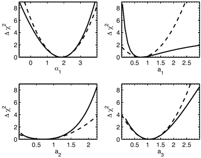
Figure 3.— Confidence levels $\Delta\chi^{2}=-2{\rm ln}(P_{\rm 1D}/P_{\rm 1D}^{\rm max})$ as a function of individual fitting parameters (except $a_{0}$). In each panel, marginalization is performed over the remaining parameters, as described in the text.

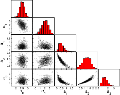
Figure 4.— Random samples drawn from $P_{\rm tot}$ ($l_{\rm max}=100$) with the MCMC algorithm.

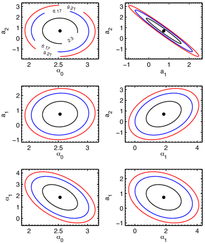
Figure 5.— Confidence levels in 2D projections of the parameter space. The contours $\chi^{2}=2.3$, 6.17, and $9.21$ correspond to $68\%$, $95.4\%$ and $99\%$ confidence levels, respectively. In each panel, marginalization in performed over the remaining 3 parameters.

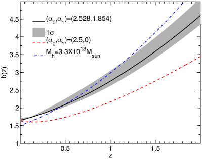
Figure 6.— The biasing factor of radio galaxies as a function of redshift. Solid curve is obtained with the ML estimates for $\alpha_{0}$ and $\alpha_{1}$ and the shaded area represents $\pm 1\sigma$ deviation from the ML $\alpha_{1}$ (marginalization over $\alpha_{0}$ is performed). For reference, the red dashed and blue dash-dot lines show, respectively, the $b(z)$ for $\alpha_{1}=0$ and for halos of mass $3.3\times 10^{13}M_{\odot}$.

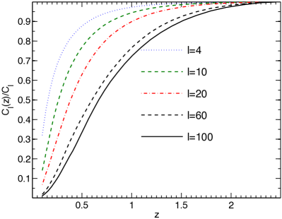
Figure 7.— The fractional contribution to $C_{l}$ resulting from integration from redshift zero to $z$. The full $C_{l}$ is obtained with $z=3.5$. Only 5 values of $l$ presented, as indicated in the figure.

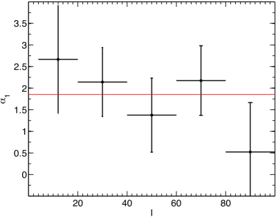
Figure 8.— The inferred $\alpha_{1}$ from $C_{l}$ for different cuts on $l$. The horizontal bar spans the $l$ values used to obtain each point and the error bar represents the corresponding $1\sigma$ marginalized error.

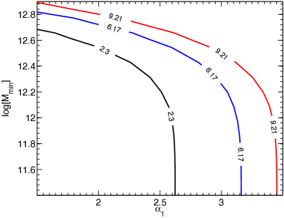
Figure 9.— Confidence levels in the plane of $\alpha_{1}$ and the minimum halo mass (in solar masses) for hosting radio galaxies.

Table 1ML estimates of the model 5 parameters and the corresponding error estimates for $l_{\rm max}=100$. The Hessian (second derivatives of $-{\rm ln}P$ with respect to the fitting parameters at the MLE values) and the error covariance (inverse of the Hessian) are also listed.

	$\alpha_{0}$	$\alpha_{1}$	$a_{1}$	$a_{2}$	$a_{3}$
	$2.529^{+0.184}_{-0.184}$	$1.854^{+0.708}_{-0.761}$	$0.739^{+1.077}_{-0.382}$	$0.705^{+0.689}_{-0.649}$	$1.057^{+0.550}_{-0.506}$
	$\pm 0.197$	$\pm 0.742$	$\pm 0.572$	$\pm 0.792$	$\pm 0.531$
Hessian
$\alpha_{0}$	54.138	13.431	-80.471	-149.24	132.57
$\alpha_{1}$	13.431	6.453	-34.429	-66.526	60.32
$a_{1}$	-80.471	-34.429	344.96	610.78	-534.96
$a_{2}$	-149.24	-66.526	610.78	1203.2	-1125.2
$a_{3}$	132.57	60.32	-534.96	-1125.2	1093.8
Error covariance
$\alpha_{0}$	0.039	-0.073	0.005	-0.003	-0.001
$\alpha_{1}$	-0.073	0.550	-0.129	0.204	0.125
$a_{1}$	0.005	-0.129	0.327	-0.444	-0.290
$a_{2}$	-0.003	0.204	-0.444	0.627	0.417
$a_{3}$	-0.001	0.125	-0.290	0.417	0.282

5. consistency with luminosity function

The joint catalog of CENSORS and Hercules used here for modeling $N(z)$ contains a small number of galaxies. It is therefore interesting to test whether our model $N^{\rm model}(z)$ is consistent with a realistic luminosity function defined as the number of sources per ${\rm log}(P)$ per comoving $\rm Mpc^{3}$. We express the radio luminosity function, $\phi(P,z)$, as the sum of the star forming (SF) galaxies and AGNs luminosity functions (Mauch & Sadler, 2007), $\phi_{{}_{\rm SF}}$ and $\phi_{{}_{\rm AGN}}$. For the SF, we follow Smolcic et al. (2008) (see also Rigby et al., 2011) to write

$$\phi_{{}_{\rm SF}}(P,z)=\phi_{{}_{\rm SF}}\left(\frac{P}{(1+z)^{2.5}},0\right)$$ (21)

for $z\leq z_{\rm max}=2.5$ and $P_{*}(z)=P(z_{\rm max})$ otherwise, and we use the parametrized form in Mauch & Sadler (2007) for $\phi_{{}_{\rm SF}}$ at $z\approx 0$. In practice, the contribution of SF is small and the exact form of $\phi_{{}_{\rm SF}}$ makes little difference to our analysis here. For the AGN luminosity distribution we write

$$\phi_{{}_{\rm AGN}}(P,z)=\frac{C}{(P/P_{*})^{\alpha}+(P/P_{*})^{\beta}}\;,$$ (22)

where the redshift dependence is via $C(z)$, $P_{*}(z)$, $\alpha(z)$ and $\beta(z)$ which are expanded in a Taylor series in $y={\rm ln}(1+z)$. The coefficients of this expansion are found by satisfying the following constraints

• the observed local $z\approx 0$ AGN luminosity function (e.g. Best et al., 2014)

• the NVSS source count, $N_{s}(S)$, giving the number of sources per flux unit.

• the redshift distribution of radio with $S>7.2\rm mJy$ obtained from the 165 galaxies in Hercules and CENSORS.

There is no physical or mathematical reasoning for fixing the order of the expansion for any of the redshift dependent functions in $\phi_{{}_{\rm AGN}}$. We adopt the expansions,

$$P_{*}(z) = P_{0}+p_{1}y+p_{2}y^{2}+p_{3}y^{3}$$

$$C = C_{0}+p_{4}y+p_{5}y^{2}+p_{6}y^{3}$$

$$\alpha = \alpha_{0}+p_{7}y+p_{8}y^{2}$$

$$\beta = \beta_{0}\;.$$ (23)

Demanding that the form (22) reduces to the observed local luminosity function yields, $C=10^{-5.33}[{\rm log_{10}}P]^{-1}\rm Mpc^{-1}$, $P_{0}=10^{24.95}\rm WHz^{-1}$, $\alpha_{0}=1.66$ and $\beta_{0}=0.42$. The redshift dependence of the faint end slope, $\beta$, is poorly probed by the source count, $N_{s}(S)$ and $N(z)$. Therefore, we simply take $\beta=\beta_{0}$. For a given choice for the parameters $p_{i}$, the luminosity yields the number of sources per unit redshift per unit ${\rm log}(S)$

$$n(S,z)=4\pi D_{c}^{2}\frac{dD_{c}}{{\rm d}z}\phi(P,z)\;,$$ (24)

where $D_{c}$ is the comoving distance to redshift $z$ and $P=P(S,z)$ is the luminosity corresponding to flux $S$ computed for a $\Lambda$CDM cosmology and a power law spectral energy distribution, $\nu^{-0.8}$. Predictions for the observed quantities $N(z)$ and $N_{s}(S)$ are easily derived from $n(S,z)$. The parameters $p_{i}$ are then obtained by maximizing the likelihood for observing these quantities. Table 2 gives the parameter $p_{i}$ along with the Hessian and the error covariance matrices. In “fit 1” in the table, galaxies with redshifts $1.45<z<2$ were excluded in the $N(z)$, while “fit 2” includes those galaxies. The AGN luminosity functions for these two fits computed at $z=1$ are shown in figure 10 together with other forms taken from Best et al. (2014) and Rigby et al. (2011) (Fit 4 in their appendix D). There is a general agreement among all the curves for $P>10^{25}\rm WHz^{-1}$. Figure 2 shows the predictions from the luminosity functions derived here as the red solid (fit 1) and red dashed (fit 2) curves. There is a very nice agreement with the observations and the other approximations to $N(z)$ plotted in the figure. An impressive agreement is also found between the predicted $N_{s}(S)$ and the observations as seen in figure 11.

Table 2Parameters of luminosity function

	$p_{1}$	$p_{2}$	$p_{3}$	$p_{4}$	$p_{5}$	$p_{6}$	$p_{7}$	$p_{8}$
Fit 1	0.15	3.3	-1.0	0.34	-2.33	0.56	-0.9	1.36
	$\pm 0.14$	$\pm 0.31$	$\pm 0.15$	$\pm 0.11$	$\pm 0.26$	$\pm 0.13$	$\pm 0.22$	$\pm 0.32$
Fit 2	-0.183	4.32	-1.635	0.74	-3.381	1.146	-0.445	0.691
	$\pm 0.32$	$\pm 0.84$	$\pm 0.46$	$\pm 0.2$	$\pm 0.53$	$\pm 0.29$	$\pm 0.24$	$\pm 0.3$
$10^{-6}$ Hessian (for fit 1 only)
$p_{1}$	0.987	0.836	0.806	1.315	1.168	1.175	-0.003	0.001
$p_{2}$	0.836	0.716	0.698	1.085	0.971	0.985	-0.012	-0.005
$p_{3}$	0.806	0.698	0.688	1.019	0.919	0.940	-0.020	-0.011
$p_{4}$	1.315	1.085	1.019	1.910	1.664	1.647	0.037	0.028
$p_{5}$	1.168	0.971	0.919	1.664	1.459	1.451	0.024	0.019
$p_{6}$	1.175	0.985	0.940	1.645	1.451	1.451	0.015	0.014
$p_{7}$	-0.003	-0.012	-0.020	0.037	0.024	0.015	0.012	0.008
$p_{8}$	0.001	-0.005	-0.011	0.028	0.019	0.014	0.008	0.005
Error covariance (for fit 1 only)
$p_{1}$	0.018	-0.041	0.019	-0.013	0.028	-0.013	-0.004	-0.002
$p_{2}$	-0.041	0.096	-0.047	0.027	-0.065	0.032	0.022	-0.016
$p_{3}$	0.019	-0.047	0.024	-0.012	0.031	-0.016	-0.016	0.018
$p_{4}$	-0.013	0.027	-0.012	0.013	-0.029	0.014	-0.002	0.009
$p_{5}$	0.028	-0.065	0.031	-0.029	0.068	-0.034	-0.005	-0.007
$p_{6}$	-0.013	0.032	-0.016	0.014	-0.034	0.017	0.006	-0.003
$p_{7}$	-0.004	0.022	-0.016	-0.002	-0.005	0.006	0.047	-0.067
$p_{8}$	-0.002	-0.016	0.018	0.009	-0.007	-0.003	-0.067	0.106

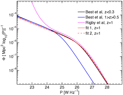
Figure 10.— Various approximations to the luminosity functions. The red solid and dashed curves (fit 1 & fit 2) correspond to the luminosity functions obtained as explained in the text.

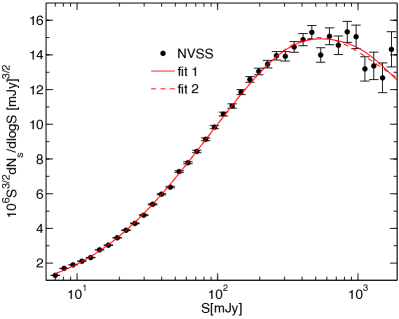
Figure 11.— Source count for the luminosity functions corresponding to fit & fit 2 compared to the NVSS observations.

6. Summary and Discussion

We have found a mild evidence ($\alpha_{1}>0$ at the 89% confidence level) for evolution in the radio activity versus stellar mass relation. If all other parameters are fixed at their ML values, i.e. assuming that they are known we get a (symmetric) $1\sigma$ error $1/\sqrt{H_{22}}=0.51$. This is the best accuracy that the clustering of the NVSS can yield for $\alpha_{1}$ if $N(z)$ and $\alpha_{0}$ are known. The constraint on $\alpha_{1}$ is obtained by using observationally motivated SHM relation (Moster et al., 2013). We have not explored the effect of systematic uncertainties in this relation which in the relevant redshift range ($z\sim 0.3-0.7$) relies on a sample of 28000 sources selected with Spitzer (Pérez‐González et al., 2008). Nonetheless, inspecting figure 10 in Coupon et al. (2015) shows that the Moster et al. (2013) relation which is adopted here is in very good agreement with the majority of observations plotted in this figure. Nonetheless we cannot rule out the possibility that $\alpha_{1}>0$ may indicate that the Moster et al. (2013) SHM ratio needs to be slightly modified at $z\sim 0.5$. Another viable interpretation for $\alpha_{1}>0$, is that halos hosting radio galaxies could be more massive than halos of other galaxies of the same stellar mass. This interpretation is in line with the conclusion of Mandelbaum et al. (2009) based on small scale clustering and galaxy galaxy lensing.

The bias factor is less sensitive to the SHM since it has to yield a theoretical ${C_{l}}$ which matches the observed angular clustering within the $\Lambda$CDM model. For the ML parameters (Table 1) we find an excellent match between the theoretical and observed ${C_{l}}$. Further, estimates of $\alpha_{1}$ obtained for different cuts imposed on $l$ are consistent with ML estimate obtained from the fiducial cut. The evidence for a dependence of $\alpha_{1}$ on scale (cf. Fig. 8) is statistically insignificant.

Mandelbaum et al. (2009) examined the angular clustering of 5700 radio loud AGNs. They analyzed two point correlations at projected separations $\lower 2.15277pt\hbox{$\;\buildrel<\over{\sim}\;$}10h^{-1}\,{\rm Mpc}$ in the frame work of halo occupation modeling (e.g. Peacock & Smith, 2000; White, 2001; Zheng et al., 2004) implemented in the Millennium simulation. In contrast to our work which is restricted to large scales ($\lower 2.15277pt\hbox{$\;\buildrel>\over{\sim}\;$}50h^{-1}\,{\rm Mpc}$), their modeling depends on the division of radio galaxies as satellites and centrals. From the clustering measurement alone they obtain a mean mass of $3\times 10^{13}M_{\odot}$, for the central halos. The bias factor we infer (cf. Fig. 6) matches that of $3.3\times 10^{13}M_{\odot}$ halos, in agreement with Mandelbaum et al. (2009). It is reassuring that the two independent studies, probing different scales, yield similar halo masses. However, incorporating galaxy-galaxy lensing in addition to clustering they obtain halo masses $(1.6\pm 0.4)\times 10^{13}M_{\odot}$. Mandelbaum et al. (2009) argue that the deviation could be attributed to uncertainties in the halo modeling, which mainly affects their clustering results. In general, it seems that galaxy-galaxy lensing incorporated in halo modeling tends to push halo masses to lower values, as revealed by inspecting figure 10 in Leauthaud et al. (2012). Nonetheless, our result is independent of the halo model. The cause of the tension between the halo mass estimates based on lensing and clustering, remains obscure.

7. Acknowledgments

We thank Curtis Saxton for a thorough reading of the manuscript. This research was supported by the I-CORE Program of the Planning and Budgeting Committee, THE ISRAEL SCIENCE FOUNDATION (grants No. 1829/12 and No. 203/09), the Asher Space Research Institute, and the Munich Institute for Astro and Particle Physics (MIAPP) of the DFG cluster of excellence Origin and Structure of the Universe .

References

- Best et al. (2003) Best, P. N., Arts, J. N., Röttgering, H. J. A., et al. 2003, Monthly Notices of the Royal Astronomical Society, 346, 627
- Best et al. (2005) Best, P. N., Kauffmann, G., Heckman, T. M., et al. 2005, Monthly Notices of the Royal Astronomical Society, 362, 25
- Best et al. (2014) Best, P. N., Ker, L. M., Simpson, C., Rigby, E. E., & Sabater, J. 2014, Monthly Notices of the Royal Astronomical Society, 445, 955
- Binney & Tabor (1995) Binney, J., & Tabor, G. 1995, MNRAS, 276, 663
- Blake et al. (2004) Blake, C., Ferreira, P. G., & Borrill, J. 2004, Monthly Notices of the Royal Astronomical Society, 351, 923
- Blake & Wall (2002) Blake, C., & Wall, J. 2002, Nature, 416, 150
- Boehringer et al. (1993) Boehringer, H., Voges, W., Fabian, A. C., Edge, A. C., & Neumann, D. M. 1993, MNRAS, 264, L25
- Bower et al. (2006) Bower, R. G., Benson, a. J., Malbon, R., et al. 2006, Monthly Notices of the Royal Astronomical Society, 370, 645
- Branchesi et al. (2005) Branchesi, M., Gioia, I. M., Fanti, C., Fanti, R., & Perley, R. 2005, Astronomy and Astrophysics, 111, 32
- Brown et al. (2011) Brown, M. J. I., Jannuzi, B. T., Floyd, D. J. E., & Mould, J. R. 2011, The Astrophysical Journal Letters, 41, 5
- Carilli et al. (1994) Carilli, C. L., Perley, R. A., & Harris, D. E. 1994, MNRAS, 270, 173
- Condon et al. (1998) Condon, J. J., Cotton, W. D., Greisen, E. W., et al. 1998, AJ, 115, 1693
- Coupon et al. (2015) Coupon, J., Arnouts, S., van Waerbeke, L., et al. 2015, Monthly Notices of the Royal Astronomical Society, 449, 1352
- Croton et al. (2006) Croton, D. J., Springel, V., White, S. D. M., et al. 2006, Monthly Notices of the Royal Astronomical Society, 365, 11
- Davis et al. (2011) Davis, M., Nusser, A., Masters, K. L., et al. 2011, Monthly Notices of the Royal Astronomical Society, 413, 2906
- Donoso et al. (2010) Donoso, E., Li, C., Kauffmann, G., Best, P. N., & Heckman, T. M. 2010, Monthly Notices of the Royal Astronomical Society, 407, 1078
- Eisenstein & Hu (1998) Eisenstein, D. J., & Hu, W. 1998, ApJ, 496, 605
- Fontanot et al. (2011) Fontanot, F., Pasquali, A., De Lucia, G., et al. 2011, Monthly Notices of the Royal Astronomical Society, 413, 957
- Gorski et al. (2005) Gorski, K. M., Hivon, E., Banday, A. J., et al. 2005, The Astrophysical Journal, 622, 759
- Hill & Lilly (1991) Hill, G. J., & Lilly, S. J. 1991, The Astrophysical Journal, 367, 1
- Lacy (2000) Lacy, M. 2000, The Astrophysical Journal, 536, L1
- Leauthaud et al. (2012) Leauthaud, A., Tinker, J., Bundy, K., et al. 2012, The Astrophysical Journal, 744, 159
- Mandelbaum et al. (2009) Mandelbaum, R., Li, C., Kauffmann, G., & White, S. D. M. 2009, Monthly Notices of the Royal Astronomical Society, 393, 377
- Mauch & Sadler (2007) Mauch, T., & Sadler, E. M. 2007, Monthly Notices of the Royal Astronomical Society, 375, 931
- McLure & Dunlop (2001) McLure, R. J., & Dunlop, J. S. 2001, Monthly Notices of the Royal Astronomical Society, 321, 515
- McNamara et al. (2000) McNamara, B. R., Wise, M., Nulsen, P. E. J., et al. 2000, The Astrophysical Journal, 534, 4
- Moster et al. (2013) Moster, B. P., Naab, T., & White, S. D. M. 2013, Monthly Notices of the Royal Astronomical Society, 428, 3121
- Norberg et al. (2001) Norberg, P., Baugh, C. M., Hawkins, E., et al. 2001, Monthly Notices of the Royal Astronomical Society, 328, 64
- Nusser et al. (2014) Nusser, A., Davis, M., & Branchini, E. 2014, The Astrophysical Journal, 788, 157
- Pasquali et al. (2009) Pasquali, A., Van Den Bosch, F. C., Mo, H. J., Yang, X., & Somerville, R. 2009, Monthly Notices of the Royal Astronomical Society, 394, 38
- Passmoor et al. (2013) Passmoor, S., Cress, C., Faltenbacher, A., et al. 2013, Monthly Notices of the Royal Astronomical Society, 429, 2183
- Peacock & Nicholson (1991) Peacock, J. A., & Nicholson, D. 1991, MNRAS, 253, 307
- Peacock & Smith (2000) Peacock, J. A., & Smith, R. E. 2000, Monthly Notices of the Royal Astronomical Society, 318, 1144
- Peebles (1980) Peebles, P. J. E. 1980, The large-scale structure of the universe (Princeton University Press)
- Pérez‐González et al. (2008) Pérez‐González, P. G., Rieke, G. H., Villar, V., et al. 2008, The Astrophysical Journal, 675, 234
- Planck Collaboration et al. (2015) Planck Collaboration, Ade, P. A. R., Aghanim, N., et al. 2015, arXiv:1502.01589
- Prestage & Peacock (1988) Prestage, R. M., & Peacock, J. A. 1988, MNRAS, 230, 131
- Rigby et al. (2011) Rigby, E. E., Best, P. N., Brookes, M. H., et al. 2011, Monthly Notices of the Royal Astronomical Society, 416, 1900
- Smolcic et al. (2008) Smolcic, V., Schinnerer, E., Zamorani, G., et al. 2008, The Astrophysical Journal, 13, 9
- van Velzen et al. (2012) van Velzen, S., Falcke, H., Schellart, P., Nierstenhöfer, N., & Kampert, K.-H. 2012, Astronomy & Astrophysics, 544, A18
- Waddington et al. (2001) Waddington, I., Dunlop, J., Peacock, J., & Windhorst, R. 2001, Monthly Notices of the Royal Astronomical Society, 328, 882
- White (2001) White, M. 2001, Monthly Notices of the Royal Astronomical Society, 321, 1
- Worpel et al. (2013) Worpel, H., Brown, M. J. I., Jones, D. H., Floyd, D. J. E., & Beutler, F. 2013, The Astrophysical Journal, 772, 64
- Zehavi et al. (2011) Zehavi, I., Zheng, Z., Weinberg, D. H., et al. 2011, The Astrophysical Journal, 736, 59
- Zheng et al. (2004) Zheng, Z., Berlind, A. a., Weinberg, D. H., et al. 2004, The Astrophysical Journal, 6, 791