Surrogate Functions for Maximizing Precision at the Top

Abstract

The problem of maximizing precision at the top of a ranked list, often dubbed Precision@k (prec@k), finds relevance in myriad learning applications such as ranking, multi-label classification, and learning with severe label imbalance. However, despite its popularity, there exist significant gaps in our understanding of this problem and its associated performance measure.

The most notable of these is the lack of a convex upper bounding surrogate for prec@k. We also lack scalable perceptron and stochastic gradient descent algorithms for optimizing this performance measure. In this paper we make key contributions in these directions. At the heart of our results is a family of truly upper bounding surrogates for prec@k. These surrogates are motivated in a principled manner and enjoy attractive properties such as consistency to prec@k under various natural margin/noise conditions.

These surrogates are then used to design a class of novel perceptron algorithms for optimizing prec@k with provable mistake bounds. We also devise scalable stochastic gradient descent style methods for this problem with provable convergence bounds. Our proofs rely on novel uniform convergence bounds which require an in-depth analysis of the structural properties of prec@k and its surrogates. We conclude with experimental results comparing our algorithms with state-of-the-art cutting plane and stochastic gradient algorithms for maximizing prec@k.

1 Introduction

Ranking a given set of points or labels according to their relevance forms the core of several real-life learning systems. For instance, in classification problems with a rare-class as is the case in spam/anomaly detection, the goal is to rank the given emails/events according to their likelihood of being from the rare-class (spam/anomaly). Similarly, in multi-label classification problems, the goal is to rank the labels according to their likelihood of being relevant to a data point Tsoumakas and Katakis (2007).

The ranking of items at the top is of utmost importance in these applications and several performance measures, such as Precision@k, Average Precision and NDCG have been designed to promote accuracy at top of ranked lists. Of these, the Precision@k (prec@k) measure is especially popular in a variety of domains. Informally, prec@k counts the number of relevant items in the top-k positions of a ranked list and is widely used in domains such as binary classification Joachims (2005), multi-label classification Prabhu and Varma (2014) and ranking Le and Smola (2007).

Given its popularity, prec@k has received attention from algorithmic, as well as learning theoretic perspectives. However, there remain specific deficiencies in our understanding of this performance measure. In fact, to the best of our knowledge, there is only one known convex surrogate function for prec@k, namely, the struct-SVM surrogate due to Joachims (2005) which, as we reveal in this work, is not an upper bound on prec@k in general, and need not recover an optimal ranking even in strictly separable settings.

Our aim in this paper is to develop efficient algorithms for optimizing prec@k for ranking problems with binary relevance levels. Since the intractability of binary classification in the agnostic setting Guruswami and Raghavendra (2009) extends to prec@k, our goal would be to exploit natural notions of benign-ness usually observed in natural distributions to overcome such intractability results.

1.1 Our Contributions

We make several contributions in this paper that both, give deeper insight into the prec@k performance measure, as well as provide scalable techniques for optimizing it.

Precision@k margin: motivated by the success of margin-based frameworks in classification settings, we develop a family of margin conditions appropriate for the prec@k problem. Recall that the prec@k performance measure counts the number of relevant items at the top $k$ positions of a ranked list. The simplest of our margin notions, that we call the weak $(k,\gamma)$-margin, is said to be present if a privileged set of $k$ relevant items can be separated from all irrelevant items by a margin of $\gamma$. This is the least restrictive margin condition that allows for a perfect ranking w.r.t prec@k. Notably, it is much less restrictive than the binary classification notion of margin which requires all relevant items to be separable from all irrelevant items by a certain margin. We also propose two other notions of margin suited to our perceptron algorithms.

Surrogate functions for prec@k: we design a family of three novel surrogates for the prec@k performance measure. Our surrogates satisfy two key properties. Firstly they always upper bound the prec@k performance measure so that optimizing them promotes better performance w.r.t prec@k. Secondly, these surrogates satisfy conditional consistency in that they are consistent w.r.t. prec@k under some noise condition. We show that there exists a one-one relationship between the three prec@k margin conditions mentioned earlier and these three surrogates so that each surrogate is consistent w.r.t. prec@k under one of the margin conditions. Moreover, our discussion reveals that the three surrogates, as well as the three margin conditions, lie in a concise hierarchy.

Perceptron and SGD algorithms: using insights gained from the previous analyses, we design two perceptron-style algorithms for optimizing prec@k. Our algorithms can be shown to be a natural extension of the classical perceptron algorithm for binary classification Rosenblatt (1958). Indeed, akin to the classical perceptron, both our algorithms enjoy mistake bounds that reduce to crisp convergence bounds under the margin conditions mentioned earlier. We also design a mini-batch-style stochastic gradient descent algorithm for optimizing prec@k.

Learning theory: in order to prove convergence bounds for the SGD algorithm, and online-to-batch conversion bounds for our perceptron algorithms, we further study prec@k and its surrogates and prove uniform convergence bounds for the same. These are novel results and require an in-depth analysis into the involved structure of the prec@k performance measure and its surrogates. However, with these results in hand, we are able to establish crisp convergence bounds for the SGD algorithm, as well as generalization bounds for our perceptron algorithms.

Paper Organization: Section 2 presents the problem formulation and sets up the notation. Section 3 introduces three novel surrogates and margin conditions for prec@k and reveals the interplay between these with respect to consistency to prec@k. Section 4 presents two perceptron algorithms for prec@k and their mistake bounds, as well as a mini-batch SGD-based algorithm. Section 5 discusses uniform convergence bounds for our surrogates and their application to convergence and online-to-batch conversion bounds for our the perceptron and SGD-style algorithms. We conclude with empirical results in Section 6.

1.2 Related Work

There has been much work in the last decade in designing algorithms for bipartite ranking problems. While the earlier methods for this problem, such as RankSVM, focused on optimizing pair-wise ranking accuracy Herbrich et al. (2000); Joachims (2002); Freund et al. (2003); Burges et al. (2005), of late, there has been enormous interest in performance measures that promote good ranking performance at the top portion of the ranked list, and in ranking methods that directly optimize these measures Clémençon and Vayatis (2007); Rudin (2009); Agarwal (2011); Boyd et al. (2012); Narasimhan and Agarwal (2013a, b); Li et al. (2014).

In this work, we focus on one such evaluation measure – Precision@k, which is widely used in practice. The only prior algorithms that we are aware of that directly optimize this performance measure are a structural SVM based cutting plane method due to Joachims (2005), and an efficient stochastic implementation of the same due to Kar et al. (2014). However, as pointed out earlier, the convex surrogate used in these methods is not well-suited for prec@k.

It is also important to note that the bipartite ranking setting considered in this work is different from other popular forms of ranking such as subset or list-wise ranking settings, which arise in several information retrieval applications, where again there has been much work in optimizing performance measures that emphasize on accuracy at the top (e.g. NDCG) Valizadegan et al. (2009); Cao et al. (2007); Yue et al. (2007); Le and Smola (2007); Chakrabarti et al. (2008); Yun et al. (2014). There has also been some recent work on perceptron style ranking methods for list-wise ranking problems Chaudhuri and Tewari (2014), but these methods are tailored to optimize the NDCG and MAP measures, which are different from the prec@k measure that we consider here. Other less related works include online ranking algorithms for optimizing ranking measures in an adversarial setting with limited feedback Chaudhuri and Tewari (2015).

2 Problem Formulation and Notation

We will be presented with a set of labeled points $({\mathbf{x}}_{i},y_{i}),\ldots,({\mathbf{x}}_{n},y_{n})$, where ${\mathbf{x}}_{i}\in{\cal X}$ and $y_{i}\in\{0,1\}$. We shall use ${\mathbf{X}}$ to denote the entire dataset, ${\mathbf{X}}_{+}$ and ${\mathbf{X}}_{-}$ to denote the set of positive and negatively (null) labeled points, and ${\mathbf{y}}\in\{0,1\}^{n}$ to denote the label vector. ${\mathbf{z}}=({\mathbf{x}},y)$ shall denote a labeled data point. Our results readily extend to multi-label and ranking settings but for sake of simplicity, we focus only on bipartite ranking problems, where the goal is to rank (a subset of) positive examples above the negative ones.

Given $n$ labeled data points ${\mathbf{z}}_{1},\ldots,{\mathbf{z}}_{n}$ and a scoring function $s:{\cal X}\rightarrow{\mathbb{R}}$, let $\sigma_{s}\in S_{n}$ be the permutation that sorts points according to the scores given by $s$ i.e. $s({\mathbf{x}}_{\sigma_{s}(i)})\geq s({\mathbf{x}}_{\sigma_{s}(j)})$ for $i\leq j$. The Precision@k measure for this scoring function can then be expressed as:

$$\textup{{prec@}k}(s;\ {\mathbf{z}}_{1},\ldots,{\mathbf{z}}_{n})=\sum_{i=1}^{k}(1-{\mathbf{y}}_{\sigma_{s}(i)}).$$ (1)

Note that the above is a “loss” version of the performance measure which penalizes any top-$k$ ranked data points that have a null label. For simplicity, we will use the abbreviated notation $\textup{{prec@}k}(s):=\textup{{prec@}k}(s;\ {\mathbf{z}}_{1},\ldots,{\mathbf{z}}_{n})$. We will also use the shorthand $s_{i}=s({\mathbf{x}}_{i})$. For any label vectors ${\mathbf{y}}^{\prime},{\mathbf{y}}^{\prime\prime}\in\{0,1\}^{n}$, we define

$$\Delta({\mathbf{y}}^{\prime},{\mathbf{y}}^{\prime\prime}) =\sum_{i=1}^{n}(1-{\mathbf{y}}_{i}^{\prime}){\mathbf{y}}_{i}^{\prime\prime},$$ (2)

$$K({\mathbf{y}}^{\prime},{\mathbf{y}}^{\prime\prime}) =\sum_{i=1}^{n}{\mathbf{y}}_{i}^{\prime}{\mathbf{y}}_{i}^{\prime\prime}.$$

Let $n_{+}({\mathbf{y}}^{\prime})=K({\mathbf{y}}^{\prime},{\mathbf{y}}^{\prime})=\left\|{{\mathbf{y}}^{\prime}}\right\|_{1}$ denote the number of positives in the label vector ${\mathbf{y}}^{\prime}$ and $n_{+}=n_{+}({\mathbf{y}})$ denote the number of actual positives. Let ${\mathbf{y}}^{(s,k)}$ be the label vector that assigns the label $1$ only to the top $k$ ranked items according to the scoring function $s$. That is, ${\mathbf{y}}^{(s,k)}_{i}=1$ if $\text{if }\sigma^{-1}_{s}(i)\leq k$ and $0$ otherwise. It is easy to verify that for any scoring function $s$, $\Delta({\mathbf{y}},{\mathbf{y}}^{(s,k)})=\textup{{prec@}k}(s)$.

3 A Family of Novel Surrogates for prec@k

As prec@k is a non-convex loss function that is hard to optimize directly, it is natural to seek surrogate functions that act as a good proxy for prec@k. There will be two properties that we shall desire of such a surrogate:

1. Upper Bounding Property: the surrogate should upper bound the prec@k loss function, so that minimizing the surrogate promotes small prec@k loss.

2. Conditional Consistency: under some regularity assumptions, optimizing the surrogate should yield an optimal solution for prec@k as well.

Motivated by the above requirements, we develop a family of surrogates which upper bound the prec@k loss function and are consistent to it under certain margin/noise conditions. We note that the results of Calauzènes et al. (2012) that negate the possibility of consistent convex surrogates for ranking performance measures do not apply to our results since they are neither stated for prec@k, nor do they negate the possibility of conditional consistency.

It is notable that the seminal work of Joachims (2005) did propose a convex surrogate for prec@k, that we refer to as $\ell^{\text{struct}}_{\textup{{prec@}k}}(\cdot)$. However, as the discussion below shows, this surrogate is not even an upper bound on prec@k let alone be consistent to it. Understanding the reasons for the failure of this surrogate would be crucial in designing our own.

3.1 The Curious Case of $\ell^{\text{struct}}_{\textup{{prec@}k}}(\cdot)$

The $\ell^{\text{struct}}_{\textup{{prec@}k}}(\cdot)$ surrogate is a part of a broad class of surrogates called struct-SVM surrogates that are designed for structured output prediction problems that can have exponentially large output spaces Joachims (2005). Given a set of $n$ labeled data points, $\ell^{\text{struct}}_{\textup{{prec@}k}}(\cdot)$ is defined as

$$\max_{\begin{subarray}{c}\hat{\mathbf{y}}\in\left\{{0,1}\right\}^{n}\\ \left\|{\hat{\mathbf{y}}}\right\|_{1}=k\end{subarray}}\left\{{\Delta({\mathbf{y}},\hat{\mathbf{y}})+\sum_{i=1}^{n}\left({\hat{\mathbf{y}}_{i}-{\mathbf{y}}_{i}}\right)s_{i}}\right\}.$$ (3)

The above surrogate penalizes a scoring function if there exists a set of $k$ points with large scores (i.e. the second term is large) which are actually negatives (i.e. the first term is large). However, since the candidate labeling $\hat{\mathbf{y}}$ is restricted to labeling just $k$ points as positive whereas the true label vector ${\mathbf{y}}$ has $n_{+}$ positives, in cases where $n_{+}>k$, a non-optimal candidate labeling $\hat{\mathbf{y}}$ can exploit the remaining $n_{+}-k$ labels to hide the high scoring negative points, thus confusing the surrogate function. This indicates that this surrogate may not be an upper bound to prec@k. We refer the reader to Appendix A for an explicit example where, not only does this surrogate not upper bound prec@k, but more importantly, minimizing $\ell^{\text{struct}}_{\textup{{prec@}k}}(\cdot)$ does not produce a model that is optimal for prec@k, even in separable settings where all positives points are separated from negatives by a margin.

In the sequel, we shall propose three surrogates, all of which are consistent with prec@k under various noise/margin conditions. The surrogates, as well as the noise conditions, will be shown to form a hierarchy.

3.2 The Ramp Surrogate $\ell^{\text{ramp}}_{\textup{{prec@}k}}(\cdot)$

The key to maximizing prec@k in a bipartite ranking setting is to select a subset of $k$ relevant items and rank them at the top $k$ positions. This can happen iff the top ranked $k$ relevant items are not outranked by any irrelevant item. Thus, a surrogate must penalize a scoring function that assigns scores to irrelevant items that are higher than those of the top ranked relevant items. Our ramp surrogate $\ell^{\text{ramp}}_{\textup{{prec@}k}}(s)$ implicitly encodes this strategy:

$$\max_{\left\|{\hat{\mathbf{y}}}\right\|_{1}=k}\left\{{\Delta({\mathbf{y}},\hat{\mathbf{y}})+\sum_{i=1}^{n}\hat{\mathbf{y}}_{i}s_{i}}\right\}-\underbrace{\max_{\begin{subarray}{c}\left\|{\tilde{\mathbf{y}}}\right\|_{1}=k\\ K({\mathbf{y}},\tilde{\mathbf{y}})=k\end{subarray}}\sum_{i=1}^{n}\tilde{\mathbf{y}}_{i}s_{i}}_{(P)}.$$ (4)

The term $(P)$ contains the sum of scores of the $k$ highest scoring positives. Note that $\ell^{\text{ramp}}_{\textup{{prec@}k}}(\cdot)$ is similar to the “ramp” losses for binary classification Do et al. (2008). We now show that $\ell^{\text{ramp}}_{\textup{{prec@}k}}(\cdot)$ is indeed an upper bounding surrogate for prec@k.

Claim 1.

For any $k\leq n_{+}$ and scoring function $s$, we have $\ell^{\text{ramp}}_{\textup{{prec@}k}}(s)\geq\textup{{prec@}k}(s)$. Moreover, if $\ell^{\text{ramp}}_{\textup{{prec@}k}}(s)\leq\xi$ for a given scoring function $s$, then there necessarily exists a set $S\subset[n]$ of size at most $k$ such that for all $\|\hat{\mathbf{y}}\|_{1}=k$, we have $\sum_{i\in S}s_{i}\geq\sum_{i=1}^{n}\hat{\mathbf{y}}_{i}s_{i}+\Delta({\mathbf{y}},\hat{\mathbf{y}})-\xi.$

Proofs for this section are deferred to Appendix B. We can show that this surrogate is conditionally consistent as well. To do so, we introduce the notion of weak $(k,\gamma)$-margin.

Definition 2 (Weak $(k,\gamma)$-margin).

A set of $n$ labeled data points satisfies the weak $(k,\gamma)$-margin condition if for some scoring function $s$ and set $S_{+}\subseteq{\mathbf{X}}_{+}$ of size $k$,

$$\min_{i\in S_{+}}s_{i}-\max_{j:{\mathbf{y}}_{j}=0}s_{j}\geq\gamma.$$

Moreover, we say that the function $s$ realizes this margin. We abbreviate the weak $(k,1)$-margin condition as simply the weak $k$-margin condition.

Clearly, a dataset has a weak $(k,\gamma)$-margin iff there exist some $k$ positive points that substantially outrank all negatives. Note that this notion of margin is strictly weaker than the standard notion of margin for binary classification as it allows all but those $k$ positives to be completely mingled with the negatives. Moreover, this seems to be one of the most natural notions of margin for prec@k. The following lemma establishes that $\ell^{\text{ramp}}_{\textup{{prec@}k}}(\cdot)$ is indeed consistent w.r.t. prec@k under the weak $k$-margin condition.

Claim 3.

For any scoring function $s$ that realizes the weak $k$-margin over a dataset, $\ell^{\text{ramp}}_{\textup{{prec@}k}}(s)=\textup{{prec@}k}(s)=0$.

This suggests that $\ell^{\text{ramp}}_{\textup{{prec@}k}}(\cdot)$ is not only a tight surrogate, but tight at the optimal scoring function, i.e. $\textup{{prec@}k}(s)=0$; this along with upper bounding property implies consistency. However, it is also a non-convex function due to the term $(P)$. To obtain convex surrogates, we perform relaxations on this term by first rewriting it as follows:

$$(P)=\sum_{i=1}^{n}{\mathbf{y}}_{i}s_{i}-\underbrace{\min_{\begin{subarray}{c}\tilde{\mathbf{y}}\preceq{\mathbf{y}}\\ \left\|{\tilde{\mathbf{y}}}\right\|_{1}=n_{+}-k\end{subarray}}\sum_{i=1}^{n}\tilde{\mathbf{y}}_{i}s_{i}}_{(Q)},$$ (5)

where $\tilde{\mathbf{y}}\preceq{\mathbf{y}}$ implies that ${\mathbf{y}}_{i}=0\Rightarrow\tilde{\mathbf{y}}_{i}=0$. Thus, to convexify the surrogate $\ell^{\text{ramp}}_{\textup{{prec@}k}}(\cdot)$, we need to design a convex upper bound on $(Q)$. Notice that the term $(Q)$ contains the sum of the scores of the $n_{+}-k$ lowest ranked positive data points. This can be readily upper bounded in several ways which give us different surrogate functions.

3.3 The Max Surrogate $\ell^{\text{max}}_{\textup{{prec@}k}}(\cdot)$

An immediate convex upper bound on $(Q)$ is obtained by replacing the sum of scores of the $n_{+}-k$ lowest ranked positives with those of the highest ranked ones as follows: $(Q)\leq\max_{\begin{subarray}{c}\tilde{\mathbf{y}}\preceq(1-\hat{\mathbf{y}})\cdot{\mathbf{y}}\\ \left\|{\tilde{\mathbf{y}}}\right\|_{1}=n_{+}-k\end{subarray}}\sum_{i=1}^{n}\tilde{\mathbf{y}}_{i}s_{i}$, which gives us the $\ell^{\text{max}}_{\textup{{prec@}k}}(s)$ surrogate defined below:

$$\max_{\left\|{\hat{\mathbf{y}}}\right\|_{1}=k}\left\{{\Delta({\mathbf{y}},\hat{\mathbf{y}})+\sum_{i=1}^{n}(\hat{\mathbf{y}}_{i}-{\mathbf{y}}_{i})s_{i}+\max_{\begin{subarray}{c}\tilde{\mathbf{y}}\preceq(1-\hat{\mathbf{y}})\cdot{\mathbf{y}}\\ \left\|{\tilde{\mathbf{y}}}\right\|_{1}=n_{+}-k\end{subarray}}\sum_{i=1}^{n}\tilde{\mathbf{y}}_{i}s_{i}}\right\}.$$ (6)

The above surrogate, being a point-wise maximum over convex functions, is convex, as well as an upper bound on $\textup{{prec@}k}(s)$ since it upper bounds $\ell^{\text{ramp}}_{\textup{{prec@}k}}(s)$. This surrogate can also be shown to be consistent w.r.t. prec@k under the strong $\gamma$-margin condition defined below for $\gamma=1$.

Definition 4 (Strong $\gamma$-margin).

A set of $n$ labeled data points satisfies the $\gamma$-strong margin condition if for some scoring function $s$, $\min_{i:{\mathbf{y}}_{i}=1}s_{i}-\max_{j:{\mathbf{y}}_{j}=0}s_{j}\geq\gamma$.

We notice that the strong margin condition is actually the standard notion of binary classification margin and hence much stronger than the weak $(k,\gamma)$-margin condition. It also does not incorporate any elements of the prec@k problem. This leads us to look for tighter convex relaxations to the term (Q) that we do below.

3.4 The Avg Surrogate $\ell^{\text{avg}}_{\textup{{prec@}k}}(\cdot)$

A tighter upper bound on $(Q)$ can be obtained by replacing $(Q)$ by the average score of the false negatives. Define $C(\hat{\mathbf{y}})=\frac{n_{+}-K({\mathbf{y}},\hat{\mathbf{y}})}{n_{+}-k}$ and consider the relaxation $(Q)\leq\frac{1}{C(\hat{\mathbf{y}})}\sum_{i=1}^{n}(1-\hat{\mathbf{y}}_{i}){\mathbf{y}}_{i}s_{i}$. Combining this with (4), we get a new convex surrogate $\ell^{\text{avg}}_{\textup{{prec@}k}}(s)$ defined as:

$$\max_{\left\|{\hat{\mathbf{y}}}\right\|_{1}=k}\left\{{\Delta({\mathbf{y}},\hat{\mathbf{y}})+\sum_{i=1}^{n}s_{i}(\hat{\mathbf{y}}_{i}-{\mathbf{y}}_{i})+\frac{1}{C(\hat{\mathbf{y}})}\sum_{i=1}^{n}(1-\hat{\mathbf{y}}_{i}){\mathbf{y}}_{i}s_{i}}\right\}.$$ (7)

We refer the reader to Appendix B.4 for a proof that $\ell^{\text{avg}}_{\textup{{prec@}k}}(\cdot)$ is an upper bounding surrogate. It is notable that for $k=n_{+}$ (i.e. for the PRBEP measure), the surrogate $\ell^{\text{avg}}_{\textup{{prec@}k}}(\cdot)$ recovers Joachims’ original surrogate $\ell^{\text{struct}}_{\textup{{prec@}k}}(\cdot)$. To establish conditional consistency of this surrogate, consider the following notion of margin:

Definition 5 ($(k,\gamma)$-margin).

A set of $n$ labeled data points satisfies the $(k,\gamma)$-margin condition if for some scoring function $s$, we have, for all sets $S_{+}\subseteq{\mathbf{X}}_{+}$ of size $n_{+}-k+1$,

$$\frac{1}{n_{+}-k+1}\sum_{i\in S_{+}}s_{i}-\max_{j:{\mathbf{y}}_{j}=0}s_{j}\geq\gamma.$$

Moreover, we say that the function $s$ realizes this margin. We abbreviate the $(k,1)$-margin condition as simply the $k$-margin condition.

We can now establish the consistency of $\ell^{\text{avg}}_{\textup{{prec@}k}}(\cdot)$ under the $k$-margin condition. See Appendix B.5 for a proof.

Claim 6.

For any scoring function $s$ that realizes the $k$-margin over a dataset, $\ell^{\text{avg}}_{\textup{{prec@}k}}(s)=\textup{{prec@}k}(s)=0$.

We note that the $(k,\gamma)$-margin condition is strictly weaker than the strong $\gamma$-margin condition (Definition 4) since it still allows a non negligible fraction of the positive points to be assigned a lower score than those assigned to negatives. On the other hand, the $(k,\gamma)$-margin condition is strictly stronger than the weak $(k,\gamma)$-margin condition (Definition 2). The weak $k$-margin condition only requires one set of $k$-positives to be separated from the negatives, whereas the above margin condition at least requires the average of all positives to be separated from the negatives.

$\displaystyle\textup{{prec@}k}(s)\leq\ell^{\text{ramp}}_{\textup{{prec@}k}}(s)$ $\displaystyle\leq\ell^{\text{avg}}_{\textup{{prec@}k}}(s)$ $\displaystyle\leq\ell^{\text{max}}_{\textup{{prec@}k}}(s)$ $\displaystyle\Uparrow\ \ \ \ \ \ \$ $\displaystyle\ \ \ \ \ \ \ \ \ \ \ \Uparrow$ $\displaystyle\ \ \ \ \ \ \ \ \ \ \Uparrow$ $\displaystyle\begin{subarray}{c}\text{\small weak $(k,\gamma)$}\\ \text{\small margin}\end{subarray}$ $\displaystyle\supseteq\ \ \ \begin{subarray}{c}\text{\small$(k,\gamma)$}\\ \text{\small margin}\end{subarray}$ $\displaystyle\supseteq\begin{subarray}{c}\text{\small strong $\gamma$}\\ \text{\small margin}\end{subarray}$

Figure 1: A hierarchy among the three surrogates for prec@k and the corresponding margin conditions for conditional consistency.

As Figure 1 demonstrates, the three surrogates presented above, as well as their corresponding margin conditions, fall in a neat hierarchy. We will now use these surrogates to formulate two perceptron algorithms with mistake bounds with respect to these margin conditions.

4 Perceptron & SGD Algorithms for prec@k

We now present perceptron-style algorithms for maximizing the prec@k performance measure in bipartite ranking settings. Our algorithms work with a stream of binary labeled points and process them in mini-batches of a predetermined size $b$. Mini-batch methods have recently gained popularity and have been used to optimize ranking loss functions such as $\ell^{\text{struct}}_{\textup{{prec@}k}}(\cdot)$ as well Kar et al. (2014). It is useful to note that the requirement for mini-batches goes away in ranking and multi-label classification settings, for our algorithms can be applied to individual data points in those settings (e.g. individual queries in ranking settings).

At every time instant $t$, our algorithms receive a batch of $b$ points ${\mathbf{X}}_{t}=\left[{{\mathbf{x}}_{t}^{1},\ldots,{\mathbf{x}}_{t}^{b}}\right]$ and rank these points using the existing model. Let $\Delta_{t}$ denote the prec@k loss (equation 1) at time $t$. If $\Delta_{t}=0$ i.e. all top $k$ ranks are occupied by positive points, then the model is not updated. Otherwise, the model is updated using the false positives and negatives. For sake of simplicity, we will only look at linear models in this paper. Depending on the kind of updates we make, we get two variants of the perceptron rule for prec@k.

Our first algorithm, Perceptron@k-avg, updates the model using a combination of all the false positives and negatives (see Algorithm 1). The effect of the update is a very natural one – it explicitly boosts the scores of the positive points that failed to reach the top ranks, and attenuates the scores of the negative points that got very high scores. It is interesting to note that in the limiting case of $k=1$ and unit batch length (i.e. $b=1$), the Perceptron@k-avg update reduces to that of the standard perceptron algorithm Rosenblatt (1958); Minsky and Papert (1988) for the choice $\hat{\mathbf{y}}_{t}=\text{sign}(s_{t})$. Thus, our algorithm can be seen as a natural extension of the classical perceptron algorithm.

Algorithm 1 Perceptron@k-avg

0:  Batch length $b$

1:  ${\mathbf{w}}^{0}\leftarrow{\mathbf{0}},t\leftarrow 0$

2:  while stream not exhausted do

3:     $t\leftarrow t+1$

4:     Receive $b$ data points ${\mathbf{X}}_{t}=\left[{{\mathbf{x}}_{t}^{1},\ldots,{\mathbf{x}}_{t}^{b}}\right]$, ${\mathbf{y}}_{t}\in\{0,1\}^{b}$

5:     Calculate $s_{t}={\mathbf{w}}^{t-1}{\mathbf{X}}_{t}$ and let $\hat{\mathbf{y}}_{t}={\mathbf{y}}^{(s_{t},k)}$

6:     $\Delta_{t}\leftarrow\Delta({\mathbf{y}}_{t},\hat{\mathbf{y}}_{t})$

7:     if $\Delta_{t}=0$ then

8:        ${\mathbf{w}}^{t}\leftarrow{\mathbf{w}}^{t-1}$

9:     else

10:        $D_{t}\leftarrow\frac{\Delta_{t}}{\left\|{{\mathbf{y}}_{t}}\right\|_{1}-K({\mathbf{y}}_{t},\hat{\mathbf{y}}_{t})}$

11:        ${\mathbf{w}}^{t}\leftarrow{\mathbf{w}}^{t-1}-\sum_{i\in[b]}(1-{\mathbf{y}}_{i})\hat{\mathbf{y}}_{i}\cdot{\mathbf{x}}_{t}^{i}$ {false positives}

12:        ${\mathbf{w}}^{t}\leftarrow{\mathbf{w}}^{t}+D_{t}\cdot\sum_{i\in[b]}(1-\hat{\mathbf{y}}_{i}){\mathbf{y}}_{i}\cdot{\mathbf{x}}_{t}^{i}$ {false negatives}

13:     end if

14:  end while

15:  return ${\mathbf{w}}^{t}$

Algorithm 2 Perceptron@k-max

10:    $S_{t}\leftarrow\text{FN}(s,\Delta_{t})$

11:    ${\mathbf{w}}^{t}\leftarrow{\mathbf{w}}^{t-1}-\sum_{i\in[b]}(1-{\mathbf{y}}_{i})\hat{\mathbf{y}}_{i}\cdot{\mathbf{x}}_{t}^{i}$ {false positives}

12:    ${\mathbf{w}}^{t}\leftarrow{\mathbf{w}}^{t}+\sum_{i\in S_{t}}{\mathbf{x}}_{t}^{i}$ {top ranked false negatives}

Algorithm 3 SGD@k-avg

0:  Batch length $b$, step lengths $\eta_{t}$, feasible set ${\cal W}$

0:  A model $\bar{\mathbf{w}}\in{\cal W}$

1:  ${\mathbf{w}}^{0}\leftarrow{\mathbf{0}},t\leftarrow 0$

2:  while stream not exhausted do

3:     $t\leftarrow t+1$

4:     Receive $b$ data points ${\mathbf{X}}_{t}=\left[{{\mathbf{x}}_{t}^{1},\ldots,{\mathbf{x}}_{t}^{b}}\right]$, ${\mathbf{y}}_{t}\in\{0,1\}^{b}$

5:     Set ${\mathbf{g}}_{t}\in\partial_{\mathbf{w}}\ell^{\text{avg}}_{\textup{{prec@}k}}({\mathbf{w}}_{t-1};{\mathbf{X}}_{t},{\mathbf{y}}_{t})${See Algorithm 4}

6:     ${\mathbf{w}}_{t}\leftarrow\Pi_{\cal W}\left[{{\mathbf{w}}_{t-1}-\eta_{t}\cdot{\mathbf{g}}_{t}}\right]${project onto set ${\cal W}$}

7:  end while

8:  return $\bar{\mathbf{w}}=\frac{1}{t}\sum_{\tau=1}^{t}{\mathbf{w}}_{\tau}$

Algorithm 4 Subgradient calculation for $\ell^{\text{avg}}_{\textup{{prec@}k}}(\cdot)$

0:  A model ${\mathbf{w}}_{\text{in}}$, $n$ data points ${\mathbf{X}},{\mathbf{y}}$, parameter $k$

0:  A subgradient ${\mathbf{g}}\in\partial_{\mathbf{w}}\ell^{\text{avg}}_{\textup{{prec@}k}}({\mathbf{w}}_{\text{in}};{\mathbf{X}},{\mathbf{y}})$

1:  Sort pos. and neg. points separately in dec. order of scores assigned by ${\mathbf{w}}_{\text{in}}$ i.e. $s_{1}^{+}\geq\ldots\geq s_{n_{+}}^{+}$ and $s_{1}^{-}\geq\ldots\geq s_{n_{-}}^{-}$

2:  for $k^{\prime}=0\rightarrow k$ do

3:     $D_{k^{\prime}}\leftarrow\frac{k-k^{\prime}}{n_{+}-k^{\prime}}$

4:     $\Delta_{k^{\prime}}\leftarrow k-k^{\prime}-D_{k^{\prime}}\sum_{i=k^{\prime}+1}^{n_{+}}s^{+}_{i}+\sum_{i=1}^{k-k^{\prime}}s^{-}_{i}$

5:     ${\mathbf{g}}_{k^{\prime}}\leftarrow\sum_{i=1}^{k-k^{\prime}}{\mathbf{x}}^{-}_{i}-D_{k^{\prime}}\sum_{i=k^{\prime}+1}^{n_{+}}{\mathbf{x}}^{+}_{i}$

6:  end for

7:  $k^{\ast}\leftarrow\arg\max_{k^{\prime}}\Delta_{k^{\prime}}$

8:  return ${\mathbf{g}}_{k^{\ast}}$

The next lemma establishes that, similar to the classical perceptron Novikoff (1962), Perceptron@k-avg also enjoys a mistake bound. Our mistake bound is stated in the most general agnostic setting with the hinge loss function replaced with our surrogate $\ell^{\text{avg}}_{\textup{{prec@}k}}(s)$. All proofs in this section are deferred to Appendix C.

Theorem 7.

Suppose $\left\|{{\mathbf{x}}_{t}^{i}}\right\|\leq R$ for all $t,i$. Let $\Delta^{C}_{T}=\sum_{t=1}^{T}\Delta_{t}$ be the cumulative mistake value observed when Algorithm 1 is executed for $T$ batches. Also, for any ${\mathbf{w}}$, let $\hat{\cal L}^{\text{avg}}_{T}({\mathbf{w}})=\sum_{t=1}^{T}\ell^{\text{avg}}_{\textup{{prec@}k}}({\mathbf{w}};{\mathbf{X}}_{t},{\mathbf{y}}_{t})$. Then we have

$$\Delta^{C}_{T}\leq\min_{{\mathbf{w}}}\ {\left({\left\|{{\mathbf{w}}}\right\|\cdot R\cdot\sqrt{4k}+\sqrt{\hat{\cal L}^{\text{avg}}_{T}({\mathbf{w}})}}\right)^{2}}.$$

Similar to the classical perceptron mistake bound Novikoff (1962), the above bound can also be reduced to a simpler convergence bound in separable settings.

Corollary 8.

Suppose a unit norm ${\mathbf{w}}^{\ast}$ exists such that the scoring function $s:{\mathbf{x}}\mapsto{\mathbf{x}}^{\top}{\mathbf{w}}^{\ast}$ realizes the $(k,\gamma)$-margin condition for all the batches, then Algorithm 1 guarantees the mistake bound: $\ \ \Delta^{C}_{T}\leq\frac{4kR^{2}}{\gamma^{2}}.$

The above result assures that, as datasets become “easier” in the sense that their $(k,\gamma)$-margin becomes larger, Perceptron@k-avg will converge to an optimal hyperplane at a faster rate. It is important to note there that the $(k,\gamma)$-margin condition is strictly weaker than the standard classification margin condition. Hence for several datasets, Perceptron@k-avg might be able to find a perfect ranking while at the same time, it might be impossible for standard binary classification techniques to find any reasonable classifier in poly-time Guruswami and Raghavendra (2009).

We note that Perceptron@k-avg performs updates with all the false negatives in the mini-batches. This raises the question as to whether sparser updates are possible as such updates would be slightly faster as well as, in high dimensional settings, ensure that the model is sparser. To this end we design the Perceptron@k-max algorithm (Algorithm 2). Perceptron@k-max differs from Perceptron@k-avg in that it performs updates using only a few of the top ranked false negatives. More specifically, for any scoring function $s$ and $m>0$, define:

$$\text{FN}(s,m)=\mathop{\arg\max}_{{S\subset{\mathbf{X}}_{t}^{+},|S|=m}}\ \sum_{i\in S}\left({1-{\mathbf{y}}^{(s,k)}_{i}}\right){\mathbf{y}}_{i}s_{i}$$

as the set of the $m$ top ranked false negatives. Perceptron@k-max makes updates only for false positives in the set $\text{FN}(s,\Delta_{t})$. Note that $\Delta_{t}$ can significantly smaller than the total number of false negatives if $k\ll n_{+}$. Perceptron@k-max also enjoys a mistake bound but with respect to the $\ell^{\text{max}}_{\textup{{prec@}k}}(\cdot)$ surrogate.

Theorem 9.

Suppose $\left\|{{\mathbf{x}}_{t}^{i}}\right\|\leq R$ for all $t,i$. Let $\Delta^{C}_{T}=\sum_{t=1}^{T}\Delta_{t}$ be the cumulative observed mistake value when Algorithm 2 is executed for $T$ batches. Also, for any ${\mathbf{w}}$, let $\hat{\cal L}^{\text{max}}_{T}({\mathbf{w}})=\sum_{t=1}^{T}\ell^{\text{max}}_{\textup{{prec@}k}}({\mathbf{w}};{\mathbf{X}}_{t},{\mathbf{y}}_{t})$. Then we have

$$\Delta^{C}_{T}\leq\min_{{\mathbf{w}}}\ {\left({\left\|{{\mathbf{w}}}\right\|\cdot R\cdot\sqrt{4k}+\sqrt{\hat{\cal L}^{\text{max}}_{T}({\mathbf{w}})}}\right)^{2}}.$$

Similar to Perceptron@k-avg, we can give a simplified mistake bound in situations where the separability condition specified by Definition 4 is satisfied.

Corollary 10.

Suppose a unit norm ${\mathbf{w}}^{\ast}$ exists such that the scoring function $s:{\mathbf{x}}\mapsto{\mathbf{x}}^{\top}{\mathbf{w}}^{\ast}$ realizes the strong $\gamma$-margin condition for all the batches, then Algorithm 2 guarantees the mistake bound: $\ \ \Delta^{C}_{T}\leq\frac{4kR^{2}}{\gamma^{2}}.$

As the strong $\gamma$-margin condition is exactly the same as the standard notion of margin for binary classification, the above bound is no stronger than the one for the classical perceptron. However, in practice, we observe that Perceptron@k-max at times outperforms even Perceptron@k-avg, even though the latter has a tighter mistake bound. This suggests that our analysis of Perceptron@k-max might not be optimal and fails to exploit latent structures that might be present in the data.

Stochastic Gradient Descent for Optimizing prec@k.
We now extend our algorithmic repertoire to include a stochastic gradient descent (SGD) algorithm for the prec@k performance measure. SGD methods are known to be very successful at optimizing large-scale empirical risk minimization (ERM) problems as they require only a few passes over the data to achieve optimal statistical accuracy.

However, SGD methods typically require access to cheap gradient estimates which are difficult to obtain for non-additive performance measures such as prec@k. This has been noticed before by several previous works Kar et al. (2014); Narasimhan et al. (2015) who propose to use mini-batch methods to overcome this problem Kar et al. (2014). By combining the $\ell^{\text{avg}}_{\textup{{prec@}k}}(\cdot)$ surrogate with mini-batch-style processing, we design SGD@k-avg (Algorithm 3), a scalable SGD algorithm for optimizing prec@k. The algorithm uses mini-batches to update the current model using gradient descent steps. The subgradient calculation for this surrogate turns out to be non-trivial and is detailed in Algorithm 4.

The task of analyzing this algorithm is made non-trivial by the fact that the gradient estimates available to SGD@k-avg via Algorithm 4 are far from being unbiased. The luxury of having unbiased gradient estimates is crucially exploited by standard SGD analyses but unfortunately, unavailable to us. To overcome this hurdle, we propose a uniform convergence based proof that, in some sense, bounds the bias in the gradient estimates.

In the following section, we present this, and many other generalization and online-to-batch conversion bounds with applications to our perceptron and SGD algorithms.

5 Generalization Bounds

In this section, we discuss novel uniform convergence (UC) bounds for our proposed surrogates. We will use these UC bounds along with the mistake bounds in Theorems 7 and 9 to prove two key results – 1) online-to-batch conversion bounds for the Perceptron@k-avg and Perceptron@k-max algorithms and, 2) a convergence guarantee for the SGD@k-avg algorithm.

To better present our generalization and convergence bounds, we use normalized versions of prec@k and the surrogates. To do so we write $k=\kappa\cdot n_{+}$ for some $\kappa\in(0,1]$ and define, for any scoring function $s$, its prec@$\kappa$ loss as:

$$\textup{{prec@}$\kappa$}(s;\ {\mathbf{z}}_{1},\ldots,{\mathbf{z}}_{n})=\frac{1}{\kappa n_{+}}\Delta({\mathbf{y}},{\mathbf{y}}^{(s,\kappa n_{+})}).$$

We will also normalize the surrogate functions $\ell^{\text{ramp}}_{\textup{{prec@}$\kappa$}}(\cdot)$, $\ell^{\text{max}}_{\textup{{prec@}$\kappa$}}(\cdot)$, and $\ell^{\text{avg}}_{\textup{{prec@}$\kappa$}}(\cdot)$ by dividing by $k=\kappa\cdot n_{+}$.

Definition 11 (Uniform Convergence).

A performance measure $\Psi:{\cal W}\times({\cal X}\times\left\{{0,1}\right\})^{n}\mapsto{\mathbb{R}}_{+}$ exhibits uniform convergence with respect to a set of predictors ${\cal W}$ if for some $\alpha(b,\delta)=\text{poly}\left({\frac{1}{b},\log\frac{1}{\delta}}\right)$, for a sample $\hat{\mathbf{z}}_{1},\ldots,\hat{\mathbf{z}}_{b}$ of size $b$ chosen i.i.d. (or uniformly without replacement) from an arbitrary population ${\mathbf{z}}_{1},\ldots,{\mathbf{z}}_{n}$, we have w.p. $1-\delta$,

$$\sup_{{\mathbf{w}}\in{\cal W}}\ \left|{\Psi({\mathbf{w}};\ {\mathbf{z}}_{1},\ldots,{\mathbf{z}}_{n})-\Psi({\mathbf{w}};\ \hat{\mathbf{z}}_{1},\ldots,\hat{\mathbf{z}}_{b})}\right|\leq\alpha(b,\delta)$$

We now state our UC bounds for prec@$\kappa$ and its surrogates. We refer the reader to Appendix D for proofs.

Theorem 12.

The loss function $\textup{{prec@}$\kappa$}(\cdot)$, as well as the surrogates $\ell^{\text{ramp}}_{\textup{{prec@}$\kappa$}}(\cdot)$, $\ell^{\text{avg}}_{\textup{{prec@}$\kappa$}}(\cdot)$ and $\ell^{\text{max}}_{\textup{{prec@}$\kappa$}}(\cdot)$, all exhibit uniform convergence at the rate $\alpha(b,\delta)={\cal O}\left({{\sqrt{\frac{1}{b}\log\frac{1}{\delta}}}}\right)$.

Recently, Kar et al. (2014) also established a similar result for the $\ell^{\text{struct}}_{\textup{{prec@}k}}(\cdot)$ surrogate. However, a very different proof technique is required to establish similar results for $\ell^{\text{max}}_{\textup{{prec@}$\kappa$}}(\cdot)$ and $\ell^{\text{avg}}_{\textup{{prec@}$\kappa$}}(\cdot)$, partly necessitated by the terms in these surrogates which depend, in a complicated manner, on the positives predicted by the candidate labeling $\hat{\mathbf{y}}$. Nevertheless, the above results allow us to establish strong online-to-batch conversion bounds for Perceptron@k-avg and Perceptron@k-max, as well as convergence rates for the SGD@k-avg method. In the following we shall assume that our data streams are composed of points chosen i.i.d. (or u.w.r.) from some fixed population ${\cal Z}$.

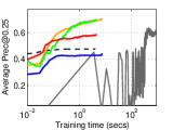
(a) PPI

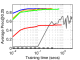
(b) Letter

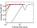
(c) Adult

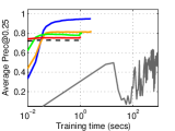
(d) IJCNN

Figure 2: A comparison of the proposed perceptron and SGD based methods with baseline methods (SVMPerf and 1PMB) on prec@0.25 maximization tasks. Perceptron@k-avg and SGD@k-avg (both based on $\ell^{\text{avg}}_{\textup{{prec@}k}}(\cdot)$) are the most consistent methods across tasks.

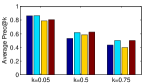
(a) KDD08

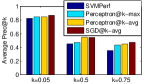
(b) PPI

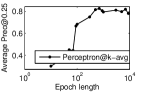
(c) KDD08

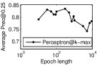
(d) KDD08

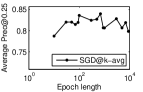
(e) KDD08

Figure 3: (a), (b): A comparison of different methods on optimizing prec@$\kappa$ for different values of $\kappa$. (c), (d), (e): The performance of the proposed perceptron and SGD methods on prec@0.25 maximization tasks with varying batch lengths $b$.

Theorem 13.

Suppose an algorithm, when fed a random stream of data points, in $T$ batches of length $b$ each, generates an ensemble of models ${\mathbf{w}}_{1},\ldots,{\mathbf{w}}_{T}$ which together suffer a cumulative mistake value of $\Delta_{T}^{C}$. Then, with probability at least $1-\delta$, we have

$$\frac{1}{T}\sum_{t=1}^{T}\textup{{prec@}$\kappa$}({\mathbf{w}}^{t};{\cal Z})\leq\frac{\Delta_{T}^{C}}{bT}+{\cal O}\left({{\sqrt{\frac{1}{b}\log\frac{T}{\delta}}}}\right).$$

The proof of this theorem follows from Theorem 12 which guarantees that w.p. $1-\delta$, $\textup{{prec@}$\kappa$}({\mathbf{w}}^{t};{\cal Z})\leq\Delta_{t}/b+{\cal O}\left({{\sqrt{\frac{1}{b}\log\frac{1}{\delta}}}}\right)$ for all $t$. Combining this with the mistake bound from Theorem 7 ensures the following generalization guarantee for the ensemble generated by Algorithm 1.

Corollary 14.

Let ${\mathbf{w}}^{1},\ldots,{\mathbf{w}}^{T}$ be the ensemble of classifiers returned by the Perceptron@k-avg algorithm on a random stream of data points and batch length $b$. Then, with probability at least $1-\delta$, for any ${\mathbf{w}}^{\ast}$ we have

$$\frac{1}{T}\sum_{t=1}^{T}\textup{{prec@}$\kappa$}({\mathbf{w}}^{t};{\cal Z})\leq\left({\sqrt{\ell^{\text{avg}}_{\textup{{prec@}$\kappa$}}({\mathbf{w}}^{\ast};{\cal Z})}+C}\right)^{2},$$

where $C={\cal O}\left({{\left\|{{\mathbf{w}}^{\ast}}\right\|R\sqrt{\frac{1}{T}}+\sqrt[4]{\frac{1}{b}\log\frac{T}{\delta}}}}\right)$.

A similar statement holds for the Perceptron@k-max algorithm with respect to the $\ell^{\text{max}}_{\textup{{prec@}$\kappa$}}(\cdot)$ surrogate as well. Using the results from Theorem 12, we can also establish the convergence rate of the SGD@k-avg algorithm.

Theorem 15.

Let $\bar{\mathbf{w}}$ be the model returned by Algorithm 3 when executed on a stream with $T$ batches of length $b$. Then with probability at least $1-\delta$, for any ${\mathbf{w}}^{\ast}\in{\cal W}$, we have

$$\ell^{\text{avg}}_{\textup{{prec@}$\kappa$}}(\bar{\mathbf{w}};{\cal Z})\leq\ell^{\text{avg}}_{\textup{{prec@}$\kappa$}}({\mathbf{w}}^{\ast};{\cal Z})+{\cal O}\left({{\sqrt{\frac{1}{b}\log\frac{T}{\delta}}}}\right)+{\cal O}\left({{\sqrt{\frac{1}{T}}}}\right)$$

The proof of this Theorem can be found in Appendix E.

6 Experiments

We shall now evaluate our methods on several benchmark datasets for binary classification problems with a rare-class.

Datasets: We evaluated our methods on 7 publicly available benchmark datasets: a) PPI, b) KDD Cup 2008, c) Letter, d) Adult, e) IJCNN, f) Covertype, and g) Cod-RNA. All datasets exhibit moderate to severe label imbalance with the KDD Cup dataset having just 0.61% positives.

Methods: We compared both perceptron algorithms, SGD@k-avg, as well as an SGD solver for the $\ell^{\text{max}}_{\textup{{prec@}k}}(\cdot)$ surrogate, with the cutting plane-based SVMPerf solver of Joachims (2005). We also compare against stochastic 1PMB solver of Kar et al. (2014). The perceptron and SGD methods were given a maximum of 25 passes over the data with a batch length of $500$. All methods were implemented in C. We used 70% of the data for training and the rest for testing. All results are averaged over $5$ random train-test splits.

Our experiments reveal three interesting insights into the problem of prec@k maximization – 1) using tighter surrogates for optimization routines is indeed beneficial, 2) the presence of a stochastic solver cannot always compensate for the use of a suboptimal surrogate, and 3) mini-batch techniques, applied with perceptron or SGD-style methods, can offer rapid convergence to accurate models.

We first timed all the methods on prec@$\kappa$ maximization tasks for $\kappa=0.25$ on various datasets (see Figure 2). Of all the methods, the cutting plane method (SVMPerf) was found to be the most expensive computationally. On the other hand, the perceptron and stochastic gradient methods, which make frequent but cheap updates, were much faster at identifying accurate solutions.

We also observed that Perceptron@k-avg and SGD@k-avg, which are based on the tight $\ell^{\text{avg}}_{\textup{{prec@}k}}(\cdot)$ surrogate, were the most consistent at converging to accurate solutions whereas Perceptron@k-max and SGD@k-max, which are based on the loose $\ell^{\text{max}}_{\textup{{prec@}k}}(\cdot)$ surrogate, showed large deviations in performance across tasks. Also, 1PMB and SVMPerf, which are based on the non upper-bounding $\ell^{\text{struct}}_{\textup{{prec@}k}}(\cdot)$ surrogate, were frequently found to converge to suboptimal solutions.

The effect of working with a tight surrogate is also clear from Figure 3 (a), (b) where the algorithms working with our novel surrogates were found to consistently outperform the SVMPerf method which works with the $\ell^{\text{struct}}_{\textup{{prec@}k}}(\cdot)$ surrogate. For these experiments, SVMPerf was allowed a runtime of up to $50\times$ of what was given to our methods after which it was terminated.

Finally, to establish the stability of our algorithms, we ran, both the perceptron, as well as the SGD algorithms with varying batch lengths (see Figure 3 (c)-(e)). We found the algorithms to be relatively stable to the setting of the batch length. To put things in perspective, all methods registered a relative variation of less than 5% in accuracies across batch lengths spanning an order of magnitude or more. We present additional experimental results in Appendix F.

Appendix A Structural SVM Surrogate for prec@k

The structural SVM surrogate for prec@k for a set of $n$ points $\{({\mathbf{x}}_{1},y_{1}),\ldots,({\mathbf{x}}_{n},y_{n})\}\in({\mathbb{R}}^{d}\times\{0,1\})^{n}$ and model $w\in{\mathbb{R}}^{d}$ can be written as $\ell_{\textup{{prec@}k}}^{\text{struct}}(w)$:

$$\max_{\begin{subarray}{c}\widehat{{\mathbf{y}}}\in\{0,1\}^{n}\\ \left\|{\widehat{\mathbf{y}}}\right\|_{1}=k\end{subarray}}\bigg{\{}1+\sum_{i=1}^{n}\widehat{{\mathbf{y}}}_{i}\bigg{(}\frac{1}{n}{\mathbf{w}}^{\top}{\mathbf{x}}_{i}-\frac{1}{k}{\mathbf{y}}_{i}\bigg{)}\,-\,\frac{1}{n}\sum_{i=1}^{n}{{\mathbf{y}}}_{i}{\mathbf{w}}^{\top}{\mathbf{x}}_{i}\bigg{\}}.$$

We shall now give a simple setting where this surrogate produces a suboptimal model.

Consider a set of 6 points in ${\mathbb{R}}\times\{0,1\}$: $\{(-1,1),(-1,1),(-2,1),(-3,0),(-3,0),(-3,0)\}$, and suppose we are interested in Prec@1. Note that the optimum model that maximizes prec@1 on these points has a positive sign. We will now show that the model $w^{*}\in{\mathbb{R}}$ that maximizes the above structural SVM surrogate on these points has a negative sign. On the contrary, let us assume that $w^{*}$ has a positive sign, and arrive at a contradiction; we shall consider the following two cases:

(i) $w^{*}>\frac{3}{2}$. It can be verified that

$$\ell_{\textup{{prec@}k}}^{\text{struct}}(w^{*}) =1+\bigg{(}\frac{1}{6}(-w^{*})-1\bigg{)}-\frac{1}{6}(-w^{*}+-w^{*}+-2w^{*})$$

$$=\frac{1}{2}w^{*}$$

On the other hand, for the model $w^{\prime}=-w^{*}$, we have

$$\ell_{\textup{{prec@}k}}^{\text{struct}}(w^{\prime}) =1+\bigg{(}\frac{1}{6}(-3w^{\prime})-0\bigg{)}-\frac{1}{6}(-w^{\prime}+-w^{\prime}+-2w^{\prime})$$

$$=1+\bigg{(}\frac{1}{6}(3w^{*})-0\bigg{)}-\frac{1}{6}(w^{*}+w^{*}+2w^{*})$$

$$=1-\frac{1}{6}w^{*}~{}<~{}\ell_{\textup{{prec@}k}}^{\text{struct}}(w^{*}),$$

where the last step follows from $w^{*}>\frac{3}{2}$; clearly, $w^{*}$ is not optimal for the structural SVM surrogate, and hence a contradiction.

(i) $w^{*}\leq\frac{3}{2}$. Here we have

$$\ell_{\textup{{prec@}k}}^{\text{struct}}(w^{*}) =1+\bigg{(}\frac{1}{6}(-3w^{*})-0\bigg{)}-\frac{1}{6}(-w^{*}+-w^{*}+-2w^{*})$$

$$=1+\frac{1}{6}w^{*}.$$

For $w^{\prime}=-w^{*}$,

$$\ell_{\textup{{prec@}k}}^{\text{struct}}(w^{\prime}) =1+\bigg{(}\frac{1}{6}(-3w^{\prime})-0\bigg{)}-\frac{1}{6}(-w^{\prime}+-w^{\prime}+-2w^{\prime})$$

$$=1+\bigg{(}\frac{1}{6}(3w^{*})-0\bigg{)}-\frac{1}{6}(w^{*}+w^{*}+2w^{*})$$

$$=1-\frac{1}{6}w^{*}~{}<~{}\ell_{\textup{{prec@}k}}^{\text{struct}}(w^{*}).$$

Here again, we have a contradiction. Notice that this surrogate can take negative values (when $w<-6$ for example) whereas prec@k is a positive valued function. This clearly indicates that this surrogate cannot upper bound prec@k. More specifically, notice that for $w<0$, we have $\textup{{prec@}k}(w)=1$, however, the above analysis demonstrates cases when $\ell_{\textup{{prec@}k}}^{\text{struct}}(w)<1$ which gives an explicit example that this surrogate is not even an upper bounding surrogate.

Appendix B Proofs of Claims from Section 3

B.1 Proof of Claim 1

Claim 1.

For any $k\leq n_{+}$ and scoring function $s$, we have

$$\ell^{\text{ramp}}_{\textup{{prec@}k}}(s)\geq\textup{{prec@}k}(s).$$

Moreover, if for some scoring function $s$, we have $\ell^{\text{ramp}}_{\textup{{prec@}k}}(s)\leq\xi$, then there necessarily exists a set $S\subset[n]$ of size at most $k$ such that for all $\left\|{\hat{\mathbf{y}}}\right\|=k$, we have

$$\sum_{i\in S}s_{i}\geq\sum_{i=1}^{n}\hat{\mathbf{y}}_{i}s_{i}+\Delta({\mathbf{y}},\hat{\mathbf{y}})-\xi.$$

Proof.

Let $\hat{\mathbf{y}}={\mathbf{y}}^{(s,k)}$ so that we have $\Delta({\mathbf{y}},\hat{\mathbf{y}})=\textup{{prec@}k}(s)$. Then we have

$$\ell^{\text{ramp}}_{\textup{{prec@}k}}(s) =\max_{\left\|{\hat{\mathbf{y}}}\right\|_{1}=k}\left\{{\Delta({\mathbf{y}},\hat{\mathbf{y}})+\sum_{i=1}^{n}\hat{\mathbf{y}}_{i}s_{i}}\right\}-{\max_{\begin{subarray}{c}\left\|{\tilde{\mathbf{y}}}\right\|_{1}=k\\ K({\mathbf{y}},\tilde{\mathbf{y}})=k\end{subarray}}\sum_{i=1}^{n}\tilde{\mathbf{y}}_{i}s_{i}}$$

$$\geq{\Delta({\mathbf{y}},\hat{\mathbf{y}})+\sum_{i=1}^{n}\hat{\mathbf{y}}_{i}s_{i}}-{\max_{\begin{subarray}{c}\left\|{\tilde{\mathbf{y}}}\right\|_{1}=k\\ K({\mathbf{y}},\tilde{\mathbf{y}})=k\end{subarray}}\sum_{i=1}^{n}\tilde{\mathbf{y}}_{i}s_{i}}$$

$$={\Delta({\mathbf{y}},\hat{\mathbf{y}})+\max_{\left\|{\tilde{\mathbf{y}}}\right\|_{1}=k}\sum_{i=1}^{n}\tilde{\mathbf{y}}_{i}s_{i}}-{\max_{\begin{subarray}{c}\left\|{\tilde{\mathbf{y}}}\right\|_{1}=k\\ K({\mathbf{y}},\tilde{\mathbf{y}})=k\end{subarray}}\sum_{i=1}^{n}\tilde{\mathbf{y}}_{i}s_{i}}$$

$$\geq\Delta({\mathbf{y}},\hat{\mathbf{y}}),$$

where the third step follows from the definition of $\hat{\mathbf{y}}$. This proves the first claim. For the second claim, suppose for some scoring function $s$, we have $\ell^{\text{ramp}}_{\textup{{prec@}k}}(s)\leq\xi$. Then if we consider $S^{\ast}$ to be the set of $k$-highest ranked positive points, then we have

$$\sum_{i\in S^{\ast}}s_{i}=\max_{\begin{subarray}{c}\left\|{\tilde{\mathbf{y}}}\right\|_{1}=k\\ K({\mathbf{y}},\tilde{\mathbf{y}})=k\end{subarray}}\sum_{i=1}^{n}\tilde{\mathbf{y}}_{i}s_{i}\geq\max_{\left\|{\hat{\mathbf{y}}}\right\|_{1}=k}\left\{{\Delta({\mathbf{y}},\hat{\mathbf{y}})+\sum_{i=1}^{n}\hat{\mathbf{y}}_{i}s_{i}}\right\}-\xi\geq\sum_{i=1}^{n}\hat{\mathbf{y}}_{i}s_{i}+\Delta({\mathbf{y}},\hat{\mathbf{y}})-\xi,$$

which proves the claim. ∎

B.2 Proof of Claim 3

Claim 3.

For any scoring function $s$ that realizes the weak $k$-margin over a dataset we have,

$$\ell^{\text{ramp}}_{\textup{{prec@}k}}(s)=\textup{{prec@}k}(s)=0.$$

Proof.

Consider a scoring function $s$ that satisfies the weak $k$-margin condition and any $\hat{\mathbf{y}}$ such that $\left\|{\hat{\mathbf{y}}}\right\|_{1}=k$. Based on the prec@k accuracy of $\hat{\mathbf{y}}$, we have the following two cases

Case 1 ($K({\mathbf{y}},\hat{\mathbf{y}})=k$): In this case we have

$$\Delta({\mathbf{y}},\hat{\mathbf{y}})+\sum_{i=1}^{n}\hat{\mathbf{y}}_{i}s_{i}-{\max_{\begin{subarray}{c}\left\|{\tilde{\mathbf{y}}}\right\|_{1}=k\\ K({\mathbf{y}},\tilde{\mathbf{y}})=k\end{subarray}}\sum_{i=1}^{n}\tilde{\mathbf{y}}_{i}s_{i}}=0+\sum_{i=1}^{n}\hat{\mathbf{y}}_{i}s_{i}-\max_{\begin{subarray}{c}\left\|{\tilde{\mathbf{y}}}\right\|_{1}=k\\ K({\mathbf{y}},\tilde{\mathbf{y}})=k\end{subarray}}\sum_{i=1}^{n}\tilde{\mathbf{y}}_{i}s_{i}\leq 0,$$

where the first step follows since $K({\mathbf{y}},\hat{\mathbf{y}})=k$ and the second step follows since $\left\|{\hat{\mathbf{y}}}\right\|_{1}=k$, as well as $K({\mathbf{y}},\hat{\mathbf{y}})=k$.

Case 2 ($K({\mathbf{y}},\hat{\mathbf{y}})=k^{\prime}<k$): In this case let $S^{\ast}$ be the set of $k$ top ranked positive points according to the scoring function $s$. Also let $S^{\ast}_{1}$ be the set of $k^{\prime}(=K({\mathbf{y}},\hat{\mathbf{y}}))$ top ranked positives and let $S^{\ast}_{2}=S^{\ast}\backslash S^{\ast}_{1}$. Then we have

$$\Delta({\mathbf{y}},\hat{\mathbf{y}})+\sum_{i=1}^{n}\hat{\mathbf{y}}_{i}s_{i}-{\max_{\begin{subarray}{c}\left\|{\tilde{\mathbf{y}}}\right\|_{1}=k\\ K({\mathbf{y}},\tilde{\mathbf{y}})=k\end{subarray}}\sum_{i=1}^{n}\tilde{\mathbf{y}}_{i}s_{i}} =\Delta({\mathbf{y}},\hat{\mathbf{y}})+\underbrace{\sum_{i=1}^{n}\hat{\mathbf{y}}_{i}{\mathbf{y}}_{i}s_{i}}_{(A)}+\sum_{i=1}^{n}\hat{\mathbf{y}}_{i}(1-{\mathbf{y}}_{i})s_{i}-{\max_{\begin{subarray}{c}\left\|{\tilde{\mathbf{y}}}\right\|_{1}=k\\ K({\mathbf{y}},\tilde{\mathbf{y}})=k\end{subarray}}\sum_{i=1}^{n}\tilde{\mathbf{y}}_{i}s_{i}}$$

$$\leq\Delta({\mathbf{y}},\hat{\mathbf{y}})+\sum_{i\in S^{\ast}_{1}}s_{i}+\underbrace{\sum_{i=1}^{n}\hat{\mathbf{y}}_{i}(1-{\mathbf{y}}_{i})s_{i}}_{(B)}-{\max_{\begin{subarray}{c}\left\|{\tilde{\mathbf{y}}}\right\|_{1}=k\\ K({\mathbf{y}},\tilde{\mathbf{y}})=k\end{subarray}}\sum_{i=1}^{n}\tilde{\mathbf{y}}_{i}s_{i}}$$

$$\leq\Delta({\mathbf{y}},\hat{\mathbf{y}})+\sum_{i\in S^{\ast}_{1}}s_{i}+\sum_{i\in S^{\ast}_{2}}s_{i}-(k-k^{\prime})-{\max_{\begin{subarray}{c}\left\|{\tilde{\mathbf{y}}}\right\|_{1}=k\\ K({\mathbf{y}},\tilde{\mathbf{y}})=k\end{subarray}}\sum_{i=1}^{n}\tilde{\mathbf{y}}_{i}s_{i}}$$

$$=k-k^{\prime}+\sum_{i\in S^{\ast}}s_{i}-(k-k^{\prime})-{\max_{\begin{subarray}{c}\left\|{\tilde{\mathbf{y}}}\right\|_{1}=k\\ K({\mathbf{y}},\tilde{\mathbf{y}})=k\end{subarray}}\sum_{i=1}^{n}\tilde{\mathbf{y}}_{i}s_{i}}$$

$$=0,$$

where the second step follows since the term $(A)$ consists of $k^{\prime}$ true positives the third step follows since the term $(B)$ contains $k-k^{\prime}$ false positives i.e. negatives and the $k$-margin condition, the fourth step follows since $\Delta({\mathbf{y}},\hat{\mathbf{y}})=k-K({\mathbf{y}},\hat{\mathbf{y}})$ and the fifth step follows since by the definition of the set $S^{\ast}$, we have

$$\sum_{i\in S^{\ast}}s_{i}=\max_{\begin{subarray}{c}\left\|{\tilde{\mathbf{y}}}\right\|_{1}=k\\ K({\mathbf{y}},\tilde{\mathbf{y}})=k\end{subarray}}\sum_{i=1}^{n}\tilde{\mathbf{y}}_{i}s_{i}.$$

In both cases, we have shown the surrogate to be non-positive. Since the performance measure prec@k cannot take negative values, this, along with the upper bounding property implies that $\textup{{prec@}k}(s)=0$ as well. This finishes the proof. ∎

B.3 A Useful Supplementary Lemma

Lemma 16.

Given a set of $n$ real numbers $x_{1}\ldots x_{n}$ and any two integers $k\leq k^{\prime}\leq n$, we have

$$\min_{|S|=k}\frac{1}{k}\sum_{i\in S}x_{i}\leq\min_{|S^{\prime}|=k^{\prime}}\frac{1}{k^{\prime}}\sum_{j\in S^{\prime}}x_{j}$$

Proof.

The above is obviously true if $k=k^{\prime}$ so we assume that $k^{\prime}>k$. Without loss of generality assume that the set is ordered in ascending order i.e. $x_{1}\leq x_{2}\leq\ldots\leq x_{n}$. Thus, the above statement is equivalent to showing that

$$\frac{1}{k}\sum_{i=1}^{k}x_{i}\leq\frac{1}{k^{\prime}}\sum_{j=1}^{k^{\prime}}x_{j}\Leftrightarrow\left({\frac{1}{k}-\frac{1}{k^{\prime}}}\right)\sum_{i=1}^{k}x_{i}\leq\frac{1}{k^{\prime}}\sum_{j=k+1}^{k^{\prime}}x_{j}\Leftrightarrow\frac{1}{k}\sum_{i=1}^{k}x_{i}\leq\frac{1}{k^{\prime}-k}\sum_{j=k+1}^{k^{\prime}}x_{j},$$

where the last inequality is true since $k-k^{\prime}>0$ and the left hand side is the average of numbers which are all smaller than the numbers whose average forms the right hand side. This proves the lemma. ∎

B.4 Proof of the Upper-bounding Property for the $\ell^{\text{avg}}_{\textup{{prec@}k}}(\cdot)$ Surrogate

Claim 17.

For any $k\leq n_{+}$ and scoring function $s$, we have

$$\ell^{\text{avg}}_{\textup{{prec@}k}}(s)\geq\textup{{prec@}k}(s).$$

Moreover, for linear scoring functions i.e. $s({\mathbf{x}}_{i})={\mathbf{w}}^{\top}{\mathbf{x}}_{i}$ for ${\mathbf{w}}\in{\cal W}$, the surrogate $\ell^{\text{avg}}_{\textup{{prec@}k}}({\mathbf{w}})$ is convex in ${\mathbf{w}}$.

Proof.

We use the fact observed before that for any scoring function, we have $\Delta({\mathbf{y}},{\mathbf{y}}^{(s,k)})=\textup{{prec@}k}(s)$. We start off by showing the second part of the claim. Recall the definition of the surrogate $\ell^{\text{avg}}_{\textup{{prec@}k}}(s)$

$$\ell^{\text{avg}}_{\textup{{prec@}k}}({\mathbf{w}})=\max_{\left\|{\hat{\mathbf{y}}}\right\|_{1}=k}\ \left\{{\Delta({\mathbf{y}},\hat{\mathbf{y}})+\sum_{i=1}^{n}(\hat{\mathbf{y}}_{i}-{\mathbf{y}}_{i})\cdot{\mathbf{w}}^{\top}{\mathbf{x}}_{i}+\frac{1}{C(\hat{\mathbf{y}})}\sum_{i=1}^{n}(1-\hat{\mathbf{y}}_{i}){\mathbf{y}}_{i}\cdot{\mathbf{w}}^{\top}{\mathbf{x}}_{i}}\right\}$$

For sake of simplicity, for any $\hat{\mathbf{y}}\in\left\{{0,1}\right\}^{n}$, define

$$\Delta(s,\hat{\mathbf{y}})=\Delta({\mathbf{y}},\hat{\mathbf{y}})+\sum_{i=1}^{n}s_{i}(\hat{\mathbf{y}}_{i}-{\mathbf{y}}_{i})+\frac{1}{C(\hat{\mathbf{y}})}\sum_{i=1}^{n}(1-\hat{\mathbf{y}}_{i}){\mathbf{y}}_{i}s_{i}.$$

The convexity of $\ell^{\text{avg}}_{\textup{{prec@}k}}({\mathbf{w}})$ follows from the observation that the inner term in the maximization is linear (hence convex) in ${\mathbf{w}}$ and the $\max$ function is convex and increasing. We now move on to prove the first part. For sake of convenience $\tilde{\mathbf{y}}={\mathbf{y}}^{(s,k)}$. Note that $\left\|{\tilde{\mathbf{y}}}\right\|_{1}=k$ by definition. This gives us

$$\ell^{\text{avg}}_{\textup{{prec@}k}}(s) = \max_{\left\|{\hat{\mathbf{y}}}\right\|_{1}=k}\Delta(s,\hat{\mathbf{y}})\geq\Delta(s,\tilde{\mathbf{y}})$$

$$= \Delta({\mathbf{y}},\tilde{\mathbf{y}})+\sum_{i=1}^{n}s_{i}(\tilde{\mathbf{y}}_{i}-{\mathbf{y}}_{i})+\frac{1}{C(\tilde{\mathbf{y}})}\sum_{i=1}^{n}(1-\tilde{\mathbf{y}}_{i}){\mathbf{y}}_{i}s_{i}$$

$$= \Delta({\mathbf{y}},\tilde{\mathbf{y}})+\sum_{i=1}^{n}s_{i}(\tilde{\mathbf{y}}_{i}(1-{\mathbf{y}}_{i})-{\mathbf{y}}_{i}(1-\tilde{\mathbf{y}}_{i}))+\frac{n_{+}-k}{n_{+}-K({\mathbf{y}},\tilde{\mathbf{y}})}\sum_{i=1}^{n}(1-\tilde{\mathbf{y}}_{i}){\mathbf{y}}_{i}s_{i}$$

$$= \Delta({\mathbf{y}},\tilde{\mathbf{y}})+\underbrace{\sum_{i=1}^{n}\tilde{\mathbf{y}}_{i}(1-{\mathbf{y}}_{i})s_{i}}_{(A)}-\underbrace{\frac{k-K({\mathbf{y}},\tilde{\mathbf{y}})}{n_{+}-K({\mathbf{y}},\tilde{\mathbf{y}})}\sum_{i=1}^{n}(1-\tilde{\mathbf{y}}_{i}){\mathbf{y}}_{i}s_{i}}_{(B)}.$$

Now define $m=\min_{\begin{subarray}{c}\tilde{\mathbf{y}}_{i}=1\\ {\mathbf{y}}_{i}=0\end{subarray}}\ s_{i}$ and $M=\max_{\begin{subarray}{c}\tilde{\mathbf{y}}_{i}=0\\ {\mathbf{y}}_{i}=1\end{subarray}}\ s_{i}$. This gives us

$$(A)=\sum_{i=1}^{n}\tilde{\mathbf{y}}_{i}(1-{\mathbf{y}}_{i})s_{i}\geq m\sum_{i=1}^{n}\tilde{\mathbf{y}}_{i}(1-{\mathbf{y}}_{i})=\Delta({\mathbf{y}},\tilde{\mathbf{y}})\cdot m,$$

and

$$(B)=\frac{k-K({\mathbf{y}},\tilde{\mathbf{y}})}{n_{+}-K({\mathbf{y}},\tilde{\mathbf{y}})}\sum_{i=1}^{n}(1-\tilde{\mathbf{y}}_{i}){\mathbf{y}}_{i}s_{i}\leq\frac{k-K({\mathbf{y}},\tilde{\mathbf{y}})}{n_{+}-K({\mathbf{y}},\tilde{\mathbf{y}})}\sum_{i=1}^{n}(1-\tilde{\mathbf{y}}_{i}){\mathbf{y}}_{i}M=(k-K({\mathbf{y}},\tilde{\mathbf{y}}))\cdot M=\Delta({\mathbf{y}},\tilde{\mathbf{y}})\cdot M.$$

However, by definition of $\tilde{\mathbf{y}}={\mathbf{y}}^{(s,k)}$, we have

$$m\geq\min_{\tilde{\mathbf{y}}=1}\ s_{i}\geq\max_{\tilde{\mathbf{y}}=0}\ s_{i}\geq M.$$

Thus we have

$$\ell^{\text{avg}}_{\textup{{prec@}k}}(s)\geq\Delta({\mathbf{y}},\tilde{\mathbf{y}})+(A)-(B)\geq\Delta({\mathbf{y}},\tilde{\mathbf{y}})(1+m-M)\geq\Delta({\mathbf{y}},\tilde{\mathbf{y}})=\textup{{prec@}k}(s)\qed$$

B.5 Proof of Claim 6

Claim 6.

For any scoring function $s$ that realizes the $k$-margin over a dataset we have,

$$\ell^{\text{avg}}_{\textup{{prec@}k}}(s)=\textup{{prec@}k}(s)=0.$$

Proof.

We shall prove that for any $\hat{\mathbf{y}}$ such that $\left\|{\hat{\mathbf{y}}}\right\|_{1}=k$, under the $k$-margin condition, we have $\Delta(s,\hat{\mathbf{y}})=0$. This will show us that $\ell^{\text{avg}}_{\textup{{prec@}k}}(s)=\max_{\left\|{\hat{\mathbf{y}}}\right\|_{1}=k}\Delta(s,\hat{\mathbf{y}})=0$. Using Claim 17 and the fact that $\textup{{prec@}k}(s)\geq 0$ will then prove the claimed result. We will analyze two cases in order to do this

Case 1 ($K({\mathbf{y}},\hat{\mathbf{y}})=k$): In this case the labeling $\hat{\mathbf{y}}$ is able to identify $k$ relevant points correctly and thus we have $C(\hat{\mathbf{y}})=1$ and we have

$$\Delta(s,\hat{\mathbf{y}})=\Delta({\mathbf{y}},\hat{\mathbf{y}})+\sum_{i=1}^{n}s_{i}(\hat{\mathbf{y}}_{i}-{\mathbf{y}}_{i})+\sum_{i=1}^{n}(1-\hat{\mathbf{y}}_{i}){\mathbf{y}}_{i}s_{i}$$

Now, since $K({\mathbf{y}},\hat{\mathbf{y}})=k$, we have $\Delta({\mathbf{y}},\hat{\mathbf{y}})=0$ which means for all $i$ such that $\hat{\mathbf{y}}_{i}=1$, we also have ${\mathbf{y}}_{i}=1$. Thus, we have $\hat{\mathbf{y}}_{i}=\hat{\mathbf{y}}_{i}{\mathbf{y}}_{i}$. Thus,

$$\Delta(s,\hat{\mathbf{y}})=0+\sum_{i=1}^{n}s_{i}(\hat{\mathbf{y}}_{i}-{\mathbf{y}}_{i})+\sum_{i=1}^{n}({\mathbf{y}}_{i}-\hat{\mathbf{y}}_{i}{\mathbf{y}}_{i})s_{i}=\sum_{i=1}^{n}s_{i}(\hat{\mathbf{y}}_{i}-{\mathbf{y}}_{i})+\sum_{i=1}^{n}({\mathbf{y}}_{i}-\hat{\mathbf{y}}_{i})s_{i}=0$$

Case 2 ($K({\mathbf{y}},\hat{\mathbf{y}})=k^{\prime}<k$): In this case, $\hat{\mathbf{y}}$ contains false positives. Thus we have

$$\Delta(s,\hat{\mathbf{y}}) = \Delta({\mathbf{y}},\hat{\mathbf{y}})+\sum_{i=1}^{n}s_{i}(\hat{\mathbf{y}}_{i}-{\mathbf{y}}_{i})+\frac{n_{+}-k}{n_{+}-k^{\prime}}\sum_{i=1}^{n}(1-\hat{\mathbf{y}}_{i}){\mathbf{y}}_{i}s_{i}$$

$$= \Delta({\mathbf{y}},\hat{\mathbf{y}})+\sum_{i=1}^{n}\hat{\mathbf{y}}_{i}(1-{\mathbf{y}}_{i})s_{i}-\frac{k-k^{\prime}}{n_{+}-k^{\prime}}\sum_{i=1}^{n}{\mathbf{y}}_{i}(1-\hat{\mathbf{y}}_{i})s_{i}$$

$$= (k-k^{\prime})\left({\underbrace{\frac{1}{k-k^{\prime}}\Delta({\mathbf{y}},\hat{\mathbf{y}})}_{(A)}+\underbrace{\frac{1}{k-k^{\prime}}\sum_{i=1}^{n}\hat{\mathbf{y}}_{i}(1-{\mathbf{y}}_{i})s_{i}}_{(B)}-\underbrace{\frac{1}{n_{+}-k^{\prime}}\sum_{i=1}^{n}{\mathbf{y}}_{i}(1-\hat{\mathbf{y}}_{i})s_{i}}_{(C)}}\right)$$

Now we have, by definition, $(A)=1$. We also have

$$(B)=\frac{1}{k-k^{\prime}}\sum_{i=1}^{n}\hat{\mathbf{y}}_{i}(1-{\mathbf{y}}_{i})s_{i}\leq\max_{j:{\mathbf{y}}_{j}=0}s_{j},$$

as well as

$$(C) = \frac{1}{n_{+}-k^{\prime}}\sum_{i=1}^{n}{\mathbf{y}}_{i}(1-\hat{\mathbf{y}}_{i})s_{i}$$

$$\geq \min_{\begin{subarray}{c}S_{+}\subseteq{\mathbf{X}}_{+}\\ |S_{+}|=n_{+}-k^{\prime}\end{subarray}}\frac{1}{n_{+}-k^{\prime}}\sum_{i\in S_{+}}{\mathbf{y}}_{i}(1-\hat{\mathbf{y}}_{i})s_{i}$$

$$\geq \min_{\begin{subarray}{c}S_{+}\subseteq{\mathbf{X}}_{+}\\ |S_{+}|=n_{+}-k+1\end{subarray}}\frac{1}{n_{+}-k+1}\sum_{i\in S_{+}}{\mathbf{y}}_{i}(1-\hat{\mathbf{y}}_{i})s_{i},$$

where the last step follows from Lemma 16 and the fact that $k^{\prime}\leq k-1$ in this case analysis. Then we have

$$\Delta(s,\hat{\mathbf{y}})=(k-k^{\prime})((A)+(B)-(C))\leq(k-k^{\prime})\left({1+\max_{j:{\mathbf{y}}_{j}=0}s_{j}-\min_{\begin{subarray}{c}S_{+}\subseteq{\mathbf{X}}_{+}\\ |S_{+}|=n_{+}-k+1\end{subarray}}\frac{1}{n_{+}-k+1}\sum_{i\in S_{+}}{\mathbf{y}}_{i}(1-\hat{\mathbf{y}}_{i})s_{i}}\right)\leq 0$$

where the last step follows because $s$ realizes the $k$-margin. Having exhausted all cases, we establish the claim. ∎

Appendix C Proofs from Section 4

C.1 Proof of Theorem 7

Theorem 7.

Suppose $\left\|{{\mathbf{x}}_{t}^{i}}\right\|\leq R$ for all $t,i$. Let $\Delta^{C}_{T}=\sum_{t=1}^{T}\Delta_{t}$ be the cumulative observed mistake values when Algorithm 1 is run. Also, for any predictor ${\mathbf{w}}$, let $\hat{\cal L}_{T}({\mathbf{w}})=\sum_{t=1}^{T}\ell^{\text{avg}}_{\textup{{prec@}k}}({\mathbf{w}};{\mathbf{X}}_{t},{\mathbf{y}}_{t})$. Then we have

$$\Delta^{C}_{T}\leq\min_{{\mathbf{w}}}\ {\left({\left\|{{\mathbf{w}}}\right\|\cdot R\cdot\sqrt{4k}+\sqrt{\hat{\cal L}_{T}({\mathbf{w}})}}\right)^{2}}.$$

Proof.

We will prove the theorem using two lemmata that we state below.

Lemma 18.

For any time step $t$, we have

$$\left\|{{\mathbf{w}}_{t}}\right\|^{2}\leq\left\|{{\mathbf{w}}_{t-1}}\right\|^{2}+4kR^{2}\Delta_{t}$$

Lemma 19.

For any fixed ${\mathbf{w}}\in{\cal W}$, define $P_{t}:=\left\langle{{\mathbf{w}}_{t}},{{\mathbf{w}}}\right\rangle$. Then we have

$$P_{t}\geq P_{t-1}+\Delta_{t}-\ell^{\text{avg}}_{\textup{{prec@}k}}({\mathbf{w}};{\mathbf{X}}_{t},{\mathbf{y}}_{t}).$$

Using Lemmata 18 and 19, we can establish the mistake bound as follows. A repeated application of Lemma 19 tells us that

$$P_{T}\geq\sum_{t=1}^{T}\Delta_{t}-\sum_{t=1}^{T}\ell^{\text{avg}}_{\textup{{prec@}k}}({\mathbf{w}};{\mathbf{X}}_{t},{\mathbf{y}}_{t})=\Delta^{C}_{t}-\hat{\cal L}_{T}({\mathbf{w}}).$$

In case the right hand side is negative, we already have the result with us. In case it is positive, we can now analyze further using the Cauchy-Schwartz inequality, and a repeated application of Lemma 18. Starting from the above we have

$$\Delta_{T}^{C} \leq P_{T}+\hat{\cal L}_{T}({\mathbf{w}})$$

$$= \left\langle{{\mathbf{w}}_{T}},{{\mathbf{w}}}\right\rangle+\hat{\cal L}_{T}({\mathbf{w}})$$

$$\leq \left\|{{\mathbf{w}}_{T}}\right\|\left\|{{\mathbf{w}}}\right\|+\hat{\cal L}_{T}({\mathbf{w}})$$

$$\leq \left\|{{\mathbf{w}}}\right\|\sqrt{4kR^{2}\cdot\Delta_{T}^{C}}+\hat{\cal L}_{T}({\mathbf{w}}),$$

which gives us the desired result upon solving the quadratic inequality. We now prove the lemmata below. Note that in the following discussion, we have, for sake of brevity, used the notation $\hat{\mathbf{y}}=\hat{\mathbf{y}}_{t}={\mathbf{y}}^{({\mathbf{w}}_{t-1},k)}$.

Proof of Lemma 18.

For time steps where $\Delta_{t}=0$, the result obviously holds since ${\mathbf{w}}_{t}={\mathbf{w}}_{t-1}$. For analyzing other time steps, let ${\mathbf{v}}_{t}=D_{t}\cdot\sum_{i\in[b]}(1-\hat{\mathbf{y}}_{i}){\mathbf{y}}_{i}\cdot{\mathbf{x}}_{t}^{i}-\sum_{i\in[b]}(1-{\mathbf{y}}_{i})\hat{\mathbf{y}}_{i}\cdot{\mathbf{x}}_{t}^{i}$ so that ${\mathbf{w}}_{t}={\mathbf{w}}_{t-1}+{\mathbf{v}}_{t}$. This gives us

$$\left\|{{\mathbf{w}}_{t}}\right\|^{2}=\left\|{{\mathbf{w}}_{t-1}}\right\|^{2}+2\left\langle{{\mathbf{w}}_{t-1}},{{\mathbf{v}}_{t}}\right\rangle+\left\|{{\mathbf{v}}_{t}}\right\|^{2}.$$

Let $s_{i}={\mathbf{w}}_{t-1}^{\top}{\mathbf{x}}_{t}^{i}$. Then we have

$$\left\langle{{\mathbf{w}}_{t-1}},{{\mathbf{v}}_{t}}\right\rangle = D_{t}\cdot\sum_{i\in[b]}(1-\hat{\mathbf{y}}_{i}){\mathbf{y}}_{i}s_{i}-\sum_{i\in[b]}(1-{\mathbf{y}}_{i})\hat{\mathbf{y}}_{i}s_{i}$$

$$= \Delta_{t}\left({\underbrace{\frac{1}{\left\|{{\mathbf{y}}_{t}}\right\|_{1}-K({\mathbf{y}}_{t},\hat{\mathbf{y}}_{t})}\sum_{i\in[b]}(1-\hat{\mathbf{y}}_{i}){\mathbf{y}}_{i}s_{i}}_{(A)}-\underbrace{\frac{1}{\Delta_{t}}\sum_{i\in[b]}(1-{\mathbf{y}}_{i})\hat{\mathbf{y}}_{i}s_{i}}_{(B)}}\right)$$

$$\leq 0,$$

where the last step follows since $(A)$ is the average of scores given to the false negatives and $(B)$ is the average of scores given to the false positives and by the definition of $\hat{\mathbf{y}}_{t}$, since false negatives are assigned scores less than false positives, we have $(A)\leq(B)$. We also have

$$\left\|{{\mathbf{v}}_{t}}\right\|^{2} = \Delta_{t}^{2}\left\|{\frac{1}{\left\|{{\mathbf{y}}_{t}}\right\|_{1}-K({\mathbf{y}}_{t},\hat{\mathbf{y}}_{t})}\cdot\sum_{i\in[b]}(1-\hat{\mathbf{y}}_{i}){\mathbf{y}}_{i}\cdot{\mathbf{x}}_{t}^{i}-\frac{1}{\Delta_{t}}\sum_{i\in[b]}(1-{\mathbf{y}}_{i})\hat{\mathbf{y}}_{i}\cdot{\mathbf{x}}_{t}^{i}}\right\|^{2}$$

$$\leq 4\Delta_{t}^{2}R^{2}\leq 4kR^{2}\Delta_{t},$$

since $\Delta_{t}\leq k$. Combining the two gives us the desired result. ∎

Proof of Lemma 19.

We prove the result using two cases. For sake of convenience, we will refer to ${\mathbf{y}}_{t}$ and $\hat{\mathbf{y}}_{t}$ as ${\mathbf{y}}$ and $\hat{\mathbf{y}}$ respectively.

Case 1 ($\Delta_{t}=0$): In this case $P_{t}=P_{t-1}$ since the model is not updated. However, since $\ell^{\text{avg}}_{\textup{{prec@}k}}({\mathbf{w}})\geq\textup{{prec@}k}({\mathbf{w}})\geq 0$ for all ${\mathbf{w}}\in{\cal W}$ (by Claim 17), we still get

$$P_{t}\geq P_{t-1}-\ell^{\text{avg}}_{\textup{{prec@}k}}({\mathbf{w}};{\mathbf{X}}_{t},{\mathbf{y}}_{t}),$$

as required.

Case 2 ($\Delta_{t}>0$): In this case we use the update to ${\mathbf{w}}_{t-1}$ to evaluate the update to $P_{t-1}$. For sake of convenience, let us use the notation $s_{i}={\mathbf{w}}^{\top}{\mathbf{x}}_{t}^{i}$. Also note that in Algorithm 1, $D_{t}=1-\frac{1}{C(\hat{\mathbf{y}})}$.

$$P_{t} = P_{t-1}-\sum_{i\in[b]}(1-{\mathbf{y}}_{i})\hat{\mathbf{y}}_{i}s_{i}+D_{t}\cdot\sum_{i\in[b]}(1-\hat{\mathbf{y}}_{i}){\mathbf{y}}_{i}s_{i}$$

$$= P_{t-1}-\sum_{i\in[b]}(1-{\mathbf{y}}_{i})\hat{\mathbf{y}}_{i}s_{i}+\left({1-\frac{1}{C(\hat{\mathbf{y}})}}\right)\sum_{i\in[b]}(1-\hat{\mathbf{y}}_{i}){\mathbf{y}}_{i}s_{i}$$

$$= P_{t-1}-\underbrace{\left({\sum_{i\in[b]}(\hat{\mathbf{y}}_{i}-{\mathbf{y}}_{i})s_{i}+\frac{1}{C(\hat{\mathbf{y}})}\sum_{i\in[b]}(1-\hat{\mathbf{y}}_{i}){\mathbf{y}}_{i}s_{i}}\right)}_{(Q)}$$

$$\geq P_{t-1}+\Delta_{t}-\ell^{\text{avg}}_{\textup{{prec@}k}}({\mathbf{w}};{\mathbf{X}}_{t},{\mathbf{y}}_{t}),$$

where the last step follows from the definition of $\ell^{\text{avg}}_{\textup{{prec@}k}}(\cdot)$ which gives us

$$\Delta_{t}+(Q) =\Delta({\mathbf{y}},\hat{\mathbf{y}})+\sum_{i\in[b]}(\hat{\mathbf{y}}_{i}-{\mathbf{y}}_{i})s_{i}+\frac{1}{C(\hat{\mathbf{y}})}\sum_{i\in[b]}(1-\hat{\mathbf{y}}_{i}){\mathbf{y}}_{i}s_{i}$$

$$\leq\max_{\left\|{\hat{\mathbf{y}}}\right\|_{1}=k}\ \left\{{\Delta({\mathbf{y}},\hat{\mathbf{y}})+\sum_{i\in[b]}s_{i}(\hat{\mathbf{y}}_{i}-{\mathbf{y}}_{i})+\frac{1}{C(\hat{\mathbf{y}})}\sum_{i\in[b]}(1-\hat{\mathbf{y}}_{i}){\mathbf{y}}_{i}s_{i}}\right\}$$

$$=\ell^{\text{avg}}_{\textup{{prec@}k}}(s)=\ell^{\text{avg}}_{\textup{{prec@}k}}({\mathbf{w}};{\mathbf{X}}_{t},{\mathbf{y}}_{t})\qed$$

This concludes the proof of the mistake bound. ∎

C.2 Proof of Theorem 9

Theorem 9.

Suppose $\left\|{{\mathbf{x}}_{t}^{i}}\right\|\leq R$ for all $t,i$. Let $\Delta^{C}_{T}=\sum_{t=1}^{T}\Delta_{t}$ be the cumulative observed mistake values when Algorithm 2 is run. Also, for any predictor ${\mathbf{w}}$, let $\hat{\cal L}^{\text{max}}_{T}({\mathbf{w}})=\sum_{t=1}^{T}\ell^{\text{max}}_{\textup{{prec@}k}}({\mathbf{w}};{\mathbf{X}}_{t},{\mathbf{y}}_{t})$. Then we have

$$\Delta^{C}_{T}\leq\min_{{\mathbf{w}}}\ {\left({\left\|{{\mathbf{w}}}\right\|\cdot R\cdot\sqrt{4k}+\sqrt{\hat{\cal L}^{\text{max}}_{T}({\mathbf{w}})}}\right)^{2}}.$$

Proof.

As before, we will prove this theorem in two parts. Lemma 18 will continue to hold in this case as well. However, we will need a modified form of Lemma 19 that we prove below. As before, we will use the notation $\hat{\mathbf{y}}=\hat{\mathbf{y}}_{t}={\mathbf{y}}^{({\mathbf{w}}_{t-1},k)}$.

Lemma 20.

For any fixed ${\mathbf{w}}\in{\cal W}$, define $P_{t}:=\left\langle{{\mathbf{w}}_{t}},{{\mathbf{w}}}\right\rangle$. Then we have

$$P_{t}\geq P_{t-1}+\Delta_{t}-\ell^{\text{max}}_{\textup{{prec@}k}}({\mathbf{w}};{\mathbf{X}}_{t},{\mathbf{y}}_{t}).$$

Using Lemmata 18 and 20, the theorem follows as before. All that remains now is to prove Lemma 20.

Proof of Lemma 20.

We prove the result using two cases as before. For sake of convenience, we will refer to ${\mathbf{y}}_{t}$ and $\hat{\mathbf{y}}_{t}$ as ${\mathbf{y}}$ and $\hat{\mathbf{y}}$ respectively.

Case 1 ($\Delta_{t}=0$): In this case $P_{t}=P_{t-1}$ since the model is not updated. However, since $\ell^{\text{max}}_{\textup{{prec@}k}}({\mathbf{w}})\geq\textup{{prec@}k}({\mathbf{w}})\geq 0$ for all ${\mathbf{w}}\in{\cal W}$ (by Claim 1), we still get

$$P_{t}\geq P_{t-1}-\ell^{\text{max}}_{\textup{{prec@}k}}({\mathbf{w}};{\mathbf{X}}_{t},{\mathbf{y}}_{t}),$$

as required.

Case 2 ($\Delta_{t}>0$): In this case we use the update to ${\mathbf{w}}_{t-1}$ to evaluate the update to $P_{t-1}$. For sake of convenience, let us use the notation $s_{i}={\mathbf{w}}^{\top}{\mathbf{x}}_{t}^{i}$. Also note that the set $S_{t}:=\text{FN}({\mathbf{w}}^{t-1},\Delta_{t})$ contains the false negatives in the top $\Delta_{t}$ positions as ranked by ${\mathbf{w}}^{t-1}$.

$$P_{t} = P_{t-1}-\sum_{i\in[b]}(1-{\mathbf{y}}_{i})\hat{\mathbf{y}}_{i}s_{i}+\sum_{i\in S_{t}}(1-\hat{\mathbf{y}}_{i}){\mathbf{y}}_{i}s_{i}$$

$$= P_{t-1}-\sum_{i\in[b]}(1-{\mathbf{y}}_{i})\hat{\mathbf{y}}_{i}s_{i}-\sum_{i\in[b]}{\mathbf{y}}_{i}\hat{\mathbf{y}}_{i}s_{i}+\sum_{i\in[b]}{\mathbf{y}}_{i}\hat{\mathbf{y}}_{i}s_{i}+\sum_{i\in S_{t}}(1-\hat{\mathbf{y}}_{i}){\mathbf{y}}_{i}s_{i}$$

$$= P_{t-1}-\sum_{i\in[b]}\hat{\mathbf{y}}_{i}s_{i}+\sum_{i\in[b]}{\mathbf{y}}_{i}\hat{\mathbf{y}}_{i}s_{i}+\sum_{i\in S_{t}}(1-\hat{\mathbf{y}}_{i}){\mathbf{y}}_{i}s_{i}$$

$$= P_{t-1}-\left({\sum_{i\in[b]}(\hat{\mathbf{y}}_{i}-{\mathbf{y}}_{i})s_{i}+\sum_{i\in[b]}(1-\hat{\mathbf{y}}_{i}){\mathbf{y}}_{i}s_{i}-\sum_{i\in S_{t}}(1-\hat{\mathbf{y}}_{i}){\mathbf{y}}_{i}s_{i}}\right)$$

$$\geq P_{t-1}-\underbrace{\left({\sum_{i\in[b]}(\hat{\mathbf{y}}_{i}-{\mathbf{y}}_{i})s_{i}+\max_{\begin{subarray}{c}\tilde{\mathbf{y}}\preceq(1-\hat{\mathbf{y}})\cdot{\mathbf{y}}\\ \left\|{\tilde{\mathbf{y}}}\right\|_{1}=n_{+}-k\end{subarray}}\sum_{i=1}^{n}\tilde{\mathbf{y}}_{i}s_{i}}\right)}_{(Q)}$$

$$\geq P_{t-1}+\Delta_{t}-\ell^{\text{max}}_{\textup{{prec@}k}}({\mathbf{w}};{\mathbf{X}}_{t},{\mathbf{y}}_{t}),$$

where the last step follows from the definition of $\ell^{\text{avg}}_{\textup{{prec@}k}}(\cdot)$ which gives us

$$\Delta_{t}+(Q) =\Delta_{t}+\sum_{i\in[b]}(\hat{\mathbf{y}}_{i}-{\mathbf{y}}_{i})s_{i}+\max_{\begin{subarray}{c}\tilde{\mathbf{y}}\preceq(1-\hat{\mathbf{y}})\cdot{\mathbf{y}}\\ \left\|{\tilde{\mathbf{y}}}\right\|_{1}=n_{+}-k\end{subarray}}\sum_{i=1}^{n}\tilde{\mathbf{y}}_{i}s_{i}$$

$$\leq\max_{\left\|{\hat{\mathbf{y}}}\right\|_{1}=k}\ \left\{{\Delta_{t}+\sum_{i\in[b]}(\hat{\mathbf{y}}_{i}-{\mathbf{y}}_{i})s_{i}+\max_{\begin{subarray}{c}\tilde{\mathbf{y}}\preceq(1-\hat{\mathbf{y}})\cdot{\mathbf{y}}\\ \left\|{\tilde{\mathbf{y}}}\right\|_{1}=n_{+}-k\end{subarray}}\sum_{i=1}^{n}\tilde{\mathbf{y}}_{i}s_{i}}\right\}$$

$$=\ell^{\text{max}}_{\textup{{prec@}k}}(s)=\ell^{\text{max}}_{\textup{{prec@}k}}({\mathbf{w}};{\mathbf{X}}_{t},{\mathbf{y}}_{t})\qed$$

This concludes the proof of the theorem. ∎

Appendix D Proof of Theorem 12

Our proof of Theorem 12 crucially utilizes the following two lemmas that helps in exploiting the structure in our surrogate functions. The first basic lemma states that the pointwise supremum of a set of Lipschitz functions is also Lipschitz.

Lemma 21.

Let $f_{1},\ldots,f_{m}$ be $m$ real valued functions $f_{i}:{\mathbb{R}}^{n}\rightarrow{\mathbb{R}}$ such that every $f_{i}$ is $1$-Lipschitz with respect to the $\left\|{\cdot}\right\|_{\infty}$ norm. Then the function

$$g({\mathbf{v}})=\max_{i\in[m]}\ f_{i}({\mathbf{v}})$$

is $1$-Lipschitz with respect to the $\left\|{\cdot}\right\|_{\infty}$ norm too.

The second lemma establishes the convergence of additive estimates over the top of ranked lists. The abstract nature of the result would allow us to apply it to a wide variety of situations and would be crucial to our analyses.

Lemma 22.

Let ${\cal V}$ be a universe with a total order $\succeq$ established on it and let ${\mathbf{v}}_{1},\ldots,{\mathbf{v}}_{n}$ be a population of $n$ items arranged in decreasing order. Let $\hat{\mathbf{v}}_{1},\ldots,\hat{\mathbf{v}}_{b}$ be a sample chosen i.i.d. (or without replacement) from the population and arranged in decreasing order as well. Then for any fixed $h:{\cal V}\rightarrow[-1,1]$ and $\kappa\in(0,1]$, we have, with probability at least $1-\delta$ over the choice of the samples,

$$\left|{\frac{1}{\left\lceil\kappa n\right\rceil}\sum_{i=1}^{\left\lceil\kappa n\right\rceil}h({\mathbf{v}}_{i})-\frac{1}{\left\lceil\kappa b\right\rceil}\sum_{i=1}^{\left\lceil\kappa b\right\rceil}h(\hat{\mathbf{v}}_{i})}\right|\leq 4\sqrt{\frac{\log\frac{2}{\delta}}{\kappa b}}$$

Theorem 12.

The performance measure $\textup{{prec@}$\kappa$}(\cdot)$, as well as the surrogates $\ell^{\text{ramp}}_{\textup{{prec@}$\kappa$}}(\cdot)$, $\ell^{\text{avg}}_{\textup{{prec@}$\kappa$}}(\cdot)$ and $\ell^{\text{max}}_{\textup{{prec@}$\kappa$}}(\cdot)$, all exhibit uniform convergence at the rate $\alpha(b,\delta)={\cal O}\left({{\sqrt{\frac{1}{b}\log\frac{1}{\delta}}}}\right)$.

We will prove the four parts of the theorem in three separate subsections below. We shall consider a population ${\mathbf{z}}_{1},\ldots,{\mathbf{z}}_{n}$ and a sample of size $b$ $\hat{\mathbf{z}}_{1},\ldots,\hat{\mathbf{z}}_{b}$ chosen uniformly at random with (i.e. i.i.d.) or without replacement. We shall let $p$ and $\hat{p}$ denote the fraction of positives in the population and the sample respectively. In the following, we shall reserve the notation $\hat{\mathbf{y}}$ for the label vector in the sample and shall use the notation $\tilde{\mathbf{y}}$ to denote candidate labellings in the definition of the surrogate.

D.1 A Uniform Convergence Bound for the $\textup{{prec@}$\kappa$}(\cdot)$ Performance Measure

We note that a point-wise convergence result for $\textup{{prec@}$\kappa$}(\cdot)$ follows simply from Lemma 22. To see this, given a population ${\mathbf{z}}_{1},\ldots,{\mathbf{z}})n$ and a fixed model ${\mathbf{w}}\in{\cal W}$, construct a parallel population using the transformation ${\mathbf{v}}_{i}\leftarrow({\mathbf{w}}^{\top}{\mathbf{x}}_{i},{\mathbf{y}}_{i})\in{\mathbb{R}}^{2}$. We order these tuples according to their first component, i.e. along the scores and use $h({\mathbf{v}}_{i})=1-{\mathbf{y}}_{i}$. Let the population be arranged such that ${\mathbf{v}}_{1}\succeq{\mathbf{v}}_{2}\succeq\ldots$. Then this gives us

$$\sum_{i=1}^{k}h({\mathbf{v}}_{i})=\sum_{i=1}^{k}(1-{\mathbf{y}}_{i})=\textup{{prec@}k}({\mathbf{y}},{\mathbf{y}}^{({\mathbf{w}},k)})=\textup{{prec@}k}({\mathbf{w}}).$$

Thus, the application of Lemma 22 gives us the following result

Lemma 23.

For any fixed model ${\mathbf{w}}\in{\cal W}$, with probability at least $1-\delta$ over the choice of $b$ samples, we have

$$\left|{\textup{{prec@}$\kappa$}({\mathbf{w}};{\mathbf{z}}_{1},\ldots,{\mathbf{z}}_{n})-\textup{{prec@}$\kappa$}({\mathbf{w}};\hat{\mathbf{z}}_{1},\ldots,\hat{\mathbf{z}}_{b})}\right|\leq{\cal O}\left({{\sqrt{\frac{1}{b}\log\frac{1}{\delta}}}}\right).$$

To prove the uniform convergence result, we will, in some sense, require a uniform version of Lemma 22. To do so we fix some notation. For any fixed $\kappa>0$, and for any ${\mathbf{w}}\in{\cal W}$, we will define $v_{\mathbf{w}}$ as the largest real number $v$ such that

$$\sum_{i=1}^{n}{\mathbb{I}}\left[{{{\mathbf{w}}^{\top}{\mathbf{x}}_{i}\geq v}}\right]=\kappa pn$$

Similarly, we will define $\hat{v}_{\mathbf{w}}$ as the largest real number $v$ such that

$$\sum_{i=1}^{b}{\mathbb{I}}\left[{{{\mathbf{w}}^{\top}\hat{\mathbf{x}}_{i}\geq v}}\right]=\kappa\hat{p}b$$

Using this notation we can redefine $\textup{{prec@}$\kappa$}(\cdot)$ on the population, as well as the sample, as

$$\textup{{prec@}$\kappa$}({\mathbf{w}};{\mathbf{z}}_{1},\ldots,{\mathbf{z}}_{n}) :=\frac{1}{\kappa pn}\sum_{i=1}^{n}{\mathbb{I}}\left[{{{\mathbf{w}}^{\top}{\mathbf{x}}\geq v_{\mathbf{w}}}}\right]\cdot{\mathbb{I}}\left[{{{\mathbf{y}}_{i}=0}}\right]$$

$$\textup{{prec@}$\kappa$}({\mathbf{w}};\hat{\mathbf{z}}_{1},\ldots,\hat{\mathbf{z}}_{b}) :=\frac{1}{\kappa\hat{p}b}\sum_{i=1}^{b}{\mathbb{I}}\left[{{{\mathbf{w}}^{\top}{\mathbf{x}}\geq\hat{v}_{\mathbf{w}}}}\right]\cdot{\mathbb{I}}\left[{{\hat{\mathbf{y}}_{i}=0}}\right]$$

We can now write

$$\sup_{{\mathbf{w}}\in{\cal W}}\left|{\textup{{prec@}$\kappa$}({\mathbf{w}};{\mathbf{z}}_{1},\ldots,{\mathbf{z}}_{n})-\textup{{prec@}$\kappa$}({\mathbf{w}};\hat{\mathbf{z}}_{1},\ldots,\hat{\mathbf{z}}_{b})}\right|$$

$$={} \sup_{{\mathbf{w}}\in{\cal W}}\left|{\frac{1}{\kappa pn}\sum_{i=1}^{n}{\mathbb{I}}\left[{{{\mathbf{w}}^{\top}{\mathbf{x}}\geq v_{\mathbf{w}}}}\right]\cdot{\mathbb{I}}\left[{{{\mathbf{y}}_{i}=0}}\right]-\frac{1}{\kappa\hat{p}b}\sum_{i=1}^{b}{\mathbb{I}}\left[{{{\mathbf{w}}^{\top}{\mathbf{x}}\geq\hat{v}_{\mathbf{w}}}}\right]\cdot{\mathbb{I}}\left[{{\hat{\mathbf{y}}_{i}=0}}\right]}\right|$$

$$\leq{} \sup_{{\mathbf{w}}\in{\cal W}}\left|{\frac{1}{\kappa pn}\sum_{i=1}^{n}{\mathbb{I}}\left[{{{\mathbf{w}}^{\top}{\mathbf{x}}\geq v_{\mathbf{w}}}}\right]\cdot{\mathbb{I}}\left[{{{\mathbf{y}}_{i}=0}}\right]-\frac{1}{\kappa\hat{p}b}\sum_{i=1}^{b}{\mathbb{I}}\left[{{{\mathbf{w}}^{\top}{\mathbf{x}}\geq v_{\mathbf{w}}}}\right]\cdot{\mathbb{I}}\left[{{\hat{\mathbf{y}}_{i}=0}}\right]}\right|$$

$$+\sup_{{\mathbf{w}}\in{\cal W}}\left|{\frac{1}{\kappa\hat{p}b}\sum_{i=1}^{b}{\mathbb{I}}\left[{{{\mathbf{w}}^{\top}{\mathbf{x}}\geq v_{\mathbf{w}}}}\right]\cdot{\mathbb{I}}\left[{{\hat{\mathbf{y}}_{i}=0}}\right]-\frac{1}{\kappa\hat{p}b}\sum_{i=1}^{b}{\mathbb{I}}\left[{{{\mathbf{w}}^{\top}{\mathbf{x}}\geq\hat{v}_{\mathbf{w}}}}\right]\cdot{\mathbb{I}}\left[{{\hat{\mathbf{y}}_{i}=0}}\right]}\right|$$

$$\leq{} \underbrace{\sup_{{\mathbf{w}}\in{\cal W},t\in{\mathbb{R}}}\left|{\frac{1}{\kappa pn}\sum_{i=1}^{n}{\mathbb{I}}\left[{{{\mathbf{w}}^{\top}{\mathbf{x}}\geq t}}\right]\cdot{\mathbb{I}}\left[{{{\mathbf{y}}_{i}=0}}\right]-\frac{1}{\kappa\hat{p}b}\sum_{i=1}^{b}{\mathbb{I}}\left[{{{\mathbf{w}}^{\top}{\mathbf{x}}\geq t}}\right]\cdot{\mathbb{I}}\left[{{\hat{\mathbf{y}}_{i}=0}}\right]}\right|}_{(A)}$$

$$+\underbrace{\sup_{{\mathbf{w}}\in{\cal W}}\left|{\frac{1}{\kappa\hat{p}b}\sum_{i=1}^{b}{\mathbb{I}}\left[{{{\mathbf{w}}^{\top}{\mathbf{x}}\geq v_{\mathbf{w}}}}\right]\cdot{\mathbb{I}}\left[{{\hat{\mathbf{y}}_{i}=0}}\right]-\frac{1}{\kappa\hat{p}b}\sum_{i=1}^{b}{\mathbb{I}}\left[{{{\mathbf{w}}^{\top}{\mathbf{x}}\geq\hat{v}_{\mathbf{w}}}}\right]\cdot{\mathbb{I}}\left[{{\hat{\mathbf{y}}_{i}=0}}\right]}\right|}_{(B)}$$

Now, using a standard VC-dimension based uniform convergence argument over the class of thresholded classifiers, we get the following result: with probability at least $1-\delta$

$$(A)\leq{\cal O}\left({{\sqrt{\frac{1}{b}\left({\log\frac{1}{\delta}+d_{\text{VC}}({\cal W})\cdot\log b}\right)}}}\right)=\tilde{\cal O}\left({{\sqrt{\frac{1}{b}\log\frac{1}{\delta}}}}\right),$$

where $d_{\text{VC}}({\cal W})$ is the VC-dimension of the set of classifiers ${\cal W}$. Moving on to bound the second term, we can use an argument similar to the one used to prove Lemma 22 to show that

$$(B) \leq\sup_{{\mathbf{w}}\in{\cal W}}\left|{\frac{1}{\kappa\hat{p}b}\sum_{i=1}^{b}{\mathbb{I}}\left[{{{\mathbf{w}}^{\top}{\mathbf{x}}\geq v_{\mathbf{w}}}}\right]-\frac{1}{\kappa\hat{p}b}\sum_{i=1}^{b}{\mathbb{I}}\left[{{{\mathbf{w}}^{\top}{\mathbf{x}}\geq\hat{v}_{\mathbf{w}}}}\right]}\right|$$

$$\leq\sup_{{\mathbf{w}}\in{\cal W}}\left|{\frac{1}{\kappa\hat{p}b}\sum_{i=1}^{b}{\mathbb{I}}\left[{{{\mathbf{w}}^{\top}{\mathbf{x}}\geq v_{\mathbf{w}}}}\right]-\kappa}\right|$$

$$\leq\sup_{{\mathbf{w}}\in{\cal W}}\left|{\frac{1}{\kappa\hat{p}b}\sum_{i=1}^{b}{\mathbb{I}}\left[{{{\mathbf{w}}^{\top}{\mathbf{x}}\geq v_{\mathbf{w}}}}\right]-\frac{1}{\kappa pn}\sum_{i=1}^{n}{\mathbb{I}}\left[{{{\mathbf{w}}^{\top}{\mathbf{x}}\geq v_{\mathbf{w}}}}\right]}\right|$$

$$\leq\tilde{\cal O}\left({{\sqrt{\frac{1}{b}\log\frac{1}{\delta}}}}\right),$$

where the last step follows from a standard VC-dimension based uniform convergence argument as before. This establishes the following uniform convergence result for the $\textup{{prec@}k}(\cdot)$ performance measure

Theorem 24.

We have, with probability at least $1-\delta$ over the choice of $b$ samples,

$$\sup_{{\mathbf{w}}\in{\cal W}}\left|{\textup{{prec@}$\kappa$}({\mathbf{w}};{\mathbf{z}}_{1},\ldots,{\mathbf{z}}_{n})-\textup{{prec@}$\kappa$}({\mathbf{w}};\hat{\mathbf{z}}_{1},\ldots,\hat{\mathbf{z}}_{b})}\right|\leq\tilde{\cal O}\left({{\sqrt{\frac{1}{b}\log\frac{1}{\delta}}}}\right).$$

D.2 A Uniform Convergence Bound for the $\ell^{\text{ramp}}_{\textup{{prec@}$\kappa$}}(\cdot)$ Surrogate

We first recall the form of the (normalized) surrogate below - note that this is a non-convex surrogate. Also recall that $k=\kappa\cdot n_{+}({\mathbf{y}})$.

$$\ell^{\text{ramp}}_{\textup{{prec@}$\kappa$}}({\mathbf{w}};\ {\mathbf{z}}_{1},\ldots,{\mathbf{z}}_{n})=\underbrace{\max_{\left\|{\tilde{\mathbf{y}}}\right\|_{1}=k}\left\{{\frac{\Delta({\mathbf{y}},\tilde{\mathbf{y}})}{k}+\frac{1}{k}\sum_{i=1}^{n}\tilde{\mathbf{y}}_{i}{\mathbf{w}}^{\top}{\mathbf{x}}_{i}}\right\}}_{\Psi_{1}({\mathbf{w}};\ {\mathbf{z}}_{1},\ldots,{\mathbf{z}}_{n})}-\underbrace{\max_{\begin{subarray}{c}\left\|{\tilde{\mathbf{y}}}\right\|_{1}=k\\ K({\mathbf{y}},\tilde{\mathbf{y}})=k\end{subarray}}\frac{1}{k}\sum_{i=1}^{n}\tilde{\mathbf{y}}_{i}{\mathbf{w}}^{\top}{\mathbf{x}}_{i}}_{\Psi_{2}({\mathbf{w}};\ {\mathbf{z}}_{1},\ldots,{\mathbf{z}}_{n})}$$

We will now show that both the functions $\Psi_{1}(\cdot)$, as well as $\Psi_{2}(\cdot)$, exhibit uniform convergence. This shall suffice to prove that $\ell^{\text{ramp}}_{\textup{{prec@}$\kappa$}}(\cdot)$ exhibits uniform convergence. To do so we shall show that the two functions exhibit pointwise convergence and that they are Lipschitz. This will allow a standard $L_{\infty}$ covering number argument Zhang [2002] to give us the required uniform convergence results.

D.2.1 A Uniform Convergence Result for $\Psi_{1}(\cdot)$

We have

$$\Psi_{1}({\mathbf{w}};\ {\mathbf{z}}_{1},\ldots,{\mathbf{z}}_{n}) =\max_{\left\|{\tilde{\mathbf{y}}}\right\|_{1}=\kappa pn}\left\{{\frac{1}{\kappa pn}\sum_{i=1}^{n}\tilde{\mathbf{y}}_{i}({\mathbf{w}}^{\top}{\mathbf{x}}_{i}-{\mathbf{y}}_{i})}\right\}+1$$

$$\Psi_{1}({\mathbf{w}};\ \hat{\mathbf{z}}_{1},\ldots,\hat{\mathbf{z}}_{b}) =\max_{\left\|{\tilde{\mathbf{y}}}\right\|_{1}=\kappa\hat{p}b}\left\{{\frac{1}{\kappa\hat{p}b}\sum_{i=1}^{b}\tilde{\mathbf{y}}_{i}({\mathbf{w}}^{\top}\hat{\mathbf{x}}_{i}-\hat{\mathbf{y}}_{i})}\right\}+1$$

An application of Corollary 29 indicates that $\Psi_{1}(\cdot)$ is Lipschitz i.e.

$$\left|{\Psi_{1}({\mathbf{w}};\ {\mathbf{z}}_{1},\ldots,{\mathbf{z}}_{n})-\Psi_{1}({\mathbf{w}}^{\prime};\ {\mathbf{z}}_{1},\ldots,{\mathbf{z}}_{n})}\right|\leq{\cal O}\left({{\left\|{{\mathbf{w}}-{\mathbf{w}}^{\prime}}\right\|_{2}}}\right).$$

Thus, all that remains is to prove pointwise convergence. We decompose the error as follows

$$\left|{\Psi_{1}({\mathbf{w}};\ {\mathbf{z}}_{1},\ldots,{\mathbf{z}}_{n})-\Psi_{1}({\mathbf{w}};\ \hat{\mathbf{z}}_{1},\ldots,\hat{\mathbf{z}}_{b})}\right|\leq{} \underbrace{\left|{\Psi_{1}({\mathbf{w}};\ {\mathbf{z}}_{1},\ldots,{\mathbf{z}}_{n})-\max_{\left\|{\tilde{\mathbf{y}}}\right\|_{1}=\kappa pb}\left\{{\frac{1}{\kappa pb}\sum_{i=1}^{b}\tilde{\mathbf{y}}_{i}({\mathbf{w}}^{\top}\hat{\mathbf{x}}_{i}-\hat{\mathbf{y}}_{i})}\right\}+1}\right|}_{(A)}$$

$$+\underbrace{\left|{\max_{\left\|{\tilde{\mathbf{y}}}\right\|_{1}=\kappa pb}\left\{{\frac{1}{\kappa pb}\sum_{i=1}^{b}\tilde{\mathbf{y}}_{i}({\mathbf{w}}^{\top}\hat{\mathbf{x}}_{i}-\hat{\mathbf{y}}_{i})}\right\}+1-\Psi_{1}({\mathbf{w}};\ \hat{\mathbf{z}}_{1},\ldots,\hat{\mathbf{z}}_{b})}\right|}_{(B)}$$

An application of Lemma 22 using ${\mathbf{v}}_{i}={\mathbf{w}}^{\top}\hat{\mathbf{x}}_{i}-\hat{\mathbf{y}}_{i}$ and $h(\cdot)$ as the identity function shows us that

$$(A)\leq{\cal O}\left({{\frac{1}{\kappa p}\sqrt{\frac{1}{b}\log\frac{1}{\delta}}}}\right).$$

To bound the residual term $(B)$, notice that an application of the Hoeffding’s inequality tells us that with probability at least $1-\delta$

$$\left|{p-\hat{p}}\right|\leq\sqrt{\frac{1}{2b}\log\frac{2}{\delta}},$$

which lets us bound the residual as follows. Assume, for sake of simplicity, that the sample data points have been ordered in decreasing order of the quantity ${\mathbf{w}}^{\top}\hat{\mathbf{x}}_{i}-{\mathbf{y}}_{i}$ as well as that $\left|{{\mathbf{w}}^{\top}{\mathbf{x}}}\right|\leq 1$ for all ${\mathbf{x}}$.

$$(B) =\left|{\max_{\left\|{\tilde{\mathbf{y}}}\right\|_{1}=\kappa pb}\left\{{\frac{1}{\kappa pb}\sum_{i=1}^{b}\tilde{\mathbf{y}}_{i}({\mathbf{w}}^{\top}\hat{\mathbf{x}}_{i}-\hat{\mathbf{y}}_{i})}\right\}-\max_{\left\|{\tilde{\mathbf{y}}}\right\|_{1}=\kappa\hat{p}b}\left\{{\frac{1}{\kappa\hat{p}b}\sum_{i=1}^{b}\tilde{\mathbf{y}}_{i}({\mathbf{w}}^{\top}\hat{\mathbf{x}}_{i}-\hat{\mathbf{y}}_{i})}\right\}}\right|$$

$$=\left|{{\frac{1}{\kappa pb}\sum_{i=1}^{\kappa pb}({\mathbf{w}}^{\top}\hat{\mathbf{x}}_{i}-\hat{\mathbf{y}}_{i})}-{\frac{1}{\kappa\hat{p}b}\sum_{i=1}^{\kappa\hat{p}b}({\mathbf{w}}^{\top}\hat{\mathbf{x}}_{i}-\hat{\mathbf{y}}_{i})}}\right|$$

$$\leq\left|{\sum_{i=1}^{\kappa\min\left\{{p,\hat{p}}\right\}b}\left({\frac{1}{\kappa pb}-\frac{1}{\kappa\hat{p}b}}\right)({\mathbf{w}}^{\top}\hat{\mathbf{x}}_{i}-\hat{\mathbf{y}}_{i})}\right|+\left|{\frac{1}{\kappa\max\left\{{p,\hat{p}}\right\}b}\sum_{i=\kappa\min\left\{{p,\hat{p}}\right\}b+1}^{\kappa\max\left\{{p,\hat{p}}\right\}b}({\mathbf{w}}^{\top}\hat{\mathbf{x}}_{i}-\hat{\mathbf{y}}_{i})}\right|$$

$$\leq\frac{2}{\kappa b}\left|{\frac{p-\hat{p}}{p\hat{p}}}\right|\cdot\kappa\min\left\{{p,\hat{p}}\right\}b+\frac{2}{\kappa\max\left\{{p,\hat{p}}\right\}b}\cdot\kappa\left|{p-\hat{p}}\right|b$$

$$=2\left|{p-\hat{p}}\right|\cdot\left({\frac{\min\left\{{p,\hat{p}}\right\}}{p\hat{p}}+\frac{1}{\max\left\{{p,\hat{p}}\right\}}}\right)$$

$$\leq\sqrt{\frac{1}{2b}\log\frac{2}{\delta}}\cdot\frac{2}{\max\left\{{p,\hat{p}}\right\}}\leq\frac{2}{p}\sqrt{\frac{1}{2b}\log\frac{2}{\delta}}$$

This establishes that for any fixed ${\mathbf{w}}\in{\cal W}$, with probability at least $1-\delta$, we have

$$\left|{\Psi_{1}({\mathbf{w}};\ {\mathbf{z}}_{1},\ldots,{\mathbf{z}}_{n})-\Psi_{1}({\mathbf{w}};\ \hat{\mathbf{z}}_{1},\ldots,\hat{\mathbf{z}}_{b})}\right|\leq{\cal O}\left({{\sqrt{\frac{1}{b}\log\frac{1}{\delta}}}}\right)$$

which concludes the uniform convergence proof.

D.2.2 A Uniform Convergence Result for $\Psi_{2}(\cdot)$

The proof follows similarly here with a direct application of Corollary 29 showing us that $\Psi_{2}(\cdot)$ is Lipschitz and an application of Lemma 22 along with the observation that $\left|{p-\hat{p}}\right|\leq\sqrt{\frac{1}{2b}\log\frac{2}{\delta}}$ similar to the discussion used above concluding the point-wise convergence proof.

The above two part argument establishes the following uniform convergence result for the $\ell^{\text{ramp}}_{\textup{{prec@}$\kappa$}}(\cdot)$ performance measure

Theorem 25.

We have, with probability at least $1-\delta$ over the choice of $b$ samples,

$$\sup_{{\mathbf{w}}\in{\cal W}}\left|{\ell^{\text{ramp}}_{\textup{{prec@}$\kappa$}}({\mathbf{w}};{\mathbf{z}}_{1},\ldots,{\mathbf{z}}_{n})-\ell^{\text{ramp}}_{\textup{{prec@}$\kappa$}}({\mathbf{w}};\hat{\mathbf{z}}_{1},\ldots,\hat{\mathbf{z}}_{b})}\right|\leq{\cal O}\left({{\sqrt{\frac{1}{b}\log\frac{1}{\delta}}}}\right).$$

D.3 A Uniform Convergence Bound for the $\ell^{\text{avg}}_{\textup{{prec@}$\kappa$}}(\cdot)$ Surrogate

This will be the most involved of the four bounds, given the intricate nature of the surrogate. We will prove this result using a series of partial results which we state below. As before, for any ${\mathbf{w}}\in{\cal W}$ and any $\tilde{\mathbf{y}}$, we define

$$\Delta({\mathbf{w}},\tilde{\mathbf{y}}) :=\frac{1}{\kappa pn}\left({\Delta({\mathbf{y}},\tilde{\mathbf{y}})+\sum_{i=1}^{n}(\tilde{\mathbf{y}}_{i}-{\mathbf{y}}_{i}){\mathbf{w}}^{\top}{\mathbf{x}}_{i}+\frac{1}{C(\tilde{\mathbf{y}})}\sum_{i=1}^{n}(1-\tilde{\mathbf{y}}_{i}){\mathbf{y}}_{i}{\mathbf{w}}^{\top}{\mathbf{x}}_{i}}\right)$$

$$\hat{\Delta}({\mathbf{w}},\tilde{\mathbf{y}}) :=\frac{1}{\kappa\hat{p}b}\left({\Delta(\hat{\mathbf{y}},\tilde{\mathbf{y}})+\sum_{i=1}^{n}(\tilde{\mathbf{y}}_{i}-\hat{\mathbf{y}}_{i}){\mathbf{w}}^{\top}\hat{\mathbf{x}}_{i}+\frac{1}{C(\tilde{\mathbf{y}})}\sum_{i=1}^{n}(1-\tilde{\mathbf{y}}_{i})\hat{\mathbf{y}}_{i}{\mathbf{w}}^{\top}\hat{\mathbf{x}}_{i}}\right)$$

Recall that we are using $\hat{\mathbf{y}}$ to denote the true labels of the sample points and $\tilde{\mathbf{y}}$ to denote the candidate labellings while defining the surrogates. We also define, for any $\beta\in[0,1]$, the following quantities

$$\Delta({\mathbf{w}},\beta) :=\max_{\begin{subarray}{c}\left\|{\tilde{\mathbf{y}}}\right\|_{1}=\kappa pn\\ K({\mathbf{y}},\tilde{\mathbf{y}})=\beta pn\end{subarray}}\left\{{\Delta({\mathbf{w}},\tilde{\mathbf{y}})}\right\}$$

$$\hat{\Delta}({\mathbf{w}},\beta) :=\max_{\begin{subarray}{c}\left\|{\tilde{\mathbf{y}}}\right\|_{1}=\kappa\hat{p}b\\ K(\hat{\mathbf{y}},\tilde{\mathbf{y}})=\beta\hat{p}b\end{subarray}}\left\{{\hat{\Delta}({\mathbf{w}},\tilde{\mathbf{y}})}\right\}$$

Note that $\beta$ denotes a target true positive rate and consequently, can only take values between $0$ and $\kappa$. Given the above, we claim the following lemmata

Lemma 26.

For every ${\mathbf{w}}$ and any $\beta,\beta^{\prime}\in[0,\kappa]$, we have

$$\left|{\Delta({\mathbf{w}},\beta)-\Delta({\mathbf{w}},\beta^{\prime})}\right|\leq{\cal O}\left({{\left|{\beta-\beta^{\prime}}\right|}}\right).$$

Lemma 27.

For any fixed $\beta$, we have, with probability at least $1-\delta$ over the choice of the sample

$$\sup_{{\mathbf{w}}\in{\cal W}}\left|{\Delta({\mathbf{w}},\beta)-\hat{\Delta}({\mathbf{w}},\beta)}\right|\leq{\cal O}\left({{\sqrt{\frac{1}{b}\log\frac{1}{\delta}}}}\right).$$

Using the above two lemmata as given, we can now prove the desired uniform convergence result for the $\ell^{\text{avg}}_{\textup{{prec@}$\kappa$}}(\cdot)$ surrogate:

Theorem 28.

With probability at least $1-\delta$ over the choice of the samples, we have

$$\sup_{{\mathbf{w}}\in{\cal W}}\left|{\ell^{\text{avg}}_{\textup{{prec@}$\kappa$}}({\mathbf{w}};{\mathbf{z}}_{1},\ldots,{\mathbf{z}}_{n})-\ell^{\text{avg}}_{\textup{{prec@}$\kappa$}}({\mathbf{w}};\hat{\mathbf{z}}_{1},\ldots,\hat{\mathbf{z}}_{b})}\right|\leq\tilde{\cal O}\left({{\sqrt{\frac{1}{b}\log\frac{1}{\delta}}}}\right).$$

Proof.

We note that given the definitions of $\Delta({\mathbf{w}},\beta)$ and $\hat{\Delta}({\mathbf{w}},\beta)$, we can redefine the performance measure as follows

$$\ell^{\text{avg}}_{\textup{{prec@}$\kappa$}}({\mathbf{w}};{\mathbf{z}}_{1},\ldots,{\mathbf{z}}_{n})=\max_{\beta\in[0,\kappa]}\Delta({\mathbf{w}},\beta)$$

We now note that for the population, the set of achievable values of true positive rates i.e. $\beta$ is

$$B=\left\{{0,\frac{1}{\kappa pn},\frac{2}{\kappa pn},\ldots,\frac{\kappa pn-1}{\kappa pn},1}\right\},$$

which correspond, respectively, to classifiers for which the number of true positives equals $\left\{{0,1,2\ldots\kappa pn-1,\kappa pn}\right\}$. Similarly, the set of achievable values of true positive rates i.e. $\beta$ for the sample is

$$\hat{B}=\left\{{0,\frac{1}{\kappa\hat{p}b},\frac{2}{\kappa\hat{p}b},\ldots,\frac{\kappa\hat{p}b-1}{\kappa\hat{p}b},1}\right\}.$$

Clearly, for any $\beta\in B$, there exists a $\pi_{\hat{B}}(\beta)\in\hat{B}$ such that

$$\left|{\pi_{\hat{B}}(\beta)-\beta}\right|\leq\frac{1}{\kappa\hat{p}b}.$$

Given this, let us define

$$\beta^{\ast}({\mathbf{w}}) =\arg\max_{\beta\in[0,\kappa]}\Delta({\mathbf{w}},\beta)$$

$$\hat{\beta}^{\ast}({\mathbf{w}}) =\arg\max_{\hat{\beta}\in[0,\kappa]}\hat{\Delta}({\mathbf{w}},\hat{\beta})$$

We shall assume, for the sake of simplicity, that $s|n$ so that $\hat{B}\subset B$. This gives us the following set of inequalities for any ${\mathbf{w}}\in{\cal W}$:

$$\Delta({\mathbf{w}},\beta^{\ast}({\mathbf{w}})) \leq\Delta({\mathbf{w}},\pi_{\hat{B}}(\beta^{\ast}({\mathbf{w}})))+\left|{\beta^{\ast}({\mathbf{w}})-\pi_{\hat{B}}(\beta^{\ast}({\mathbf{w}}))}\right|$$

$$\leq\hat{\Delta}({\mathbf{w}},\pi_{\hat{B}}(\beta^{\ast}({\mathbf{w}})))+\sup_{{\mathbf{w}}\in{\cal W}}\left|{\Delta({\mathbf{w}},\pi_{\hat{B}}(\beta^{\ast}({\mathbf{w}})))-\hat{\Delta}({\mathbf{w}},\pi_{\hat{B}}(\beta^{\ast}({\mathbf{w}})))}\right|+\frac{1}{\kappa\hat{p}b}$$

$$\leq\hat{\Delta}({\mathbf{w}},\pi_{\hat{B}}(\beta^{\ast}({\mathbf{w}})))+\sup_{{\mathbf{w}}\in{\cal W},\hat{\beta}\in\hat{B}}\left|{\Delta({\mathbf{w}},\hat{\beta})-\hat{\Delta}({\mathbf{w}},\hat{\beta})}\right|+\frac{1}{\kappa\hat{p}b}$$

$$\leq\hat{\Delta}({\mathbf{w}},\pi_{\hat{B}}(\beta^{\ast}({\mathbf{w}})))+{\cal O}\left({{\sqrt{\frac{1}{b}\log\frac{b}{\delta}}}}\right)+\frac{1}{\kappa\hat{p}b}$$

$$\leq\hat{\Delta}({\mathbf{w}},\hat{\beta}^{\ast}({\mathbf{w}}))+{\cal O}\left({{\sqrt{\frac{1}{b}\log\frac{b}{\delta}}}}\right)+\frac{1}{\kappa\hat{p}b},$$

where the first step follows from Lemma 26, the third step follows since $\pi_{\hat{B}}(\beta^{\ast}({\mathbf{w}}))\in\hat{B}$, the fourth step follows from an application of the union bound with Lemma 27 over the set of elements in $\hat{B}$ and noting $\left|{\hat{B}}\right|\leq{\cal O}\left({{b}}\right)$, and the last step follows from the optimality of $\hat{\beta}^{\ast}({\mathbf{w}})$. Similarly we can write, for any ${\mathbf{w}}\in{\cal W}$,

$$\hat{\Delta}({\mathbf{w}},\hat{\beta}^{\ast}({\mathbf{w}})) \leq\Delta({\mathbf{w}},\hat{\beta}^{\ast}({\mathbf{w}}))+{\cal O}\left({{\sqrt{\frac{1}{b}\log\frac{b}{\delta}}}}\right)$$

$$\leq\Delta({\mathbf{w}},\beta^{\ast}({\mathbf{w}}))+{\cal O}\left({{\sqrt{\frac{1}{b}\log\frac{b}{\delta}}}}\right),$$

where the first step uses Lemma 27 with a union bound over elements in $\hat{B}$ and the fact that $\hat{\beta}^{\ast}({\mathbf{w}})\in\hat{B}\subset B$ (note that this assumption is not crucial to the argument – indeed, even if $\hat{\beta}^{\ast}({\mathbf{w}})\notin B$, we would only incur an extra ${\cal O}\left({{\frac{1}{n}}}\right)$ error by an application of Lemma 26 since given the granularity of $B$, we would always be able to find a value in $B$ that is no more than ${\cal O}\left({{\frac{1}{n}}}\right)$ far from $\hat{\beta}^{\ast}({\mathbf{w}})$), and the last step uses the optimality of $\beta^{\ast}({\mathbf{w}})$. Thus, we can write

$$\sup_{{\mathbf{w}}\in{\cal W}}\left|{\ell^{\text{avg}}_{\textup{{prec@}$\kappa$}}({\mathbf{w}};{\mathbf{z}}_{1},\ldots,{\mathbf{z}}_{n})-\ell^{\text{avg}}_{\textup{{prec@}$\kappa$}}({\mathbf{w}};\hat{\mathbf{z}}_{1},\ldots,\hat{\mathbf{z}}_{b})}\right| =\sup_{{\mathbf{w}}\in{\cal W}}\left|{\Delta({\mathbf{w}},\beta^{\ast}({\mathbf{w}}))-\hat{\Delta}({\mathbf{w}},\hat{\beta}^{\ast}({\mathbf{w}}))}\right|$$

$$\leq{\cal O}\left({{\sqrt{\frac{1}{b}\log\frac{b}{\delta}}}}\right)+\frac{1}{\kappa\hat{p}b}$$

$$\leq\tilde{\cal O}\left({{\sqrt{\frac{1}{b}\log\frac{1}{\delta}}}}\right),$$

since $\hat{p}\geq\Omega\left({{1}}\right)$ with probability at least $1-\delta$. Thus, all we are left is to prove Lemmata 26 and 27 which we do below. To proceed with the proofs, we first write the form of $\Delta({\mathbf{w}},\beta)$ for a fixed ${\mathbf{w}}$ and $\beta$ and simplify the expression for ease of further analysis. We shall assume, for sake of simplicity, that $\beta pn,\kappa pn,\beta\hat{p}b$, and $\kappa\hat{p}b$ are all integers.

$$\Delta({\mathbf{w}},\beta) =\max_{\begin{subarray}{c}\left\|{\tilde{\mathbf{y}}}\right\|_{1}=\kappa pn\\ K({\mathbf{y}},\tilde{\mathbf{y}})=\beta pn\end{subarray}}\left\{{\frac{1}{\kappa pn}\left({\Delta({\mathbf{y}},\tilde{\mathbf{y}})+\sum_{i=1}^{n}(\tilde{\mathbf{y}}_{i}-{\mathbf{y}}_{i}){\mathbf{w}}^{\top}{\mathbf{x}}_{i}+\frac{1}{C(\tilde{\mathbf{y}})}\sum_{i=1}^{n}(1-\tilde{\mathbf{y}}_{i}){\mathbf{y}}_{i}{\mathbf{w}}^{\top}{\mathbf{x}}_{i}}\right)}\right\}$$

$$=1-\frac{\beta}{\kappa}-\underbrace{\frac{1}{\kappa pn}\left({\frac{\kappa-\beta}{1-\beta}}\right)\sum_{i=1}^{n}{\mathbf{y}}_{i}{\mathbf{w}}^{\top}{\mathbf{x}}_{i}}_{A({\mathbf{w}},\beta)}+\underbrace{\max_{\begin{subarray}{c}\left\|{\tilde{\mathbf{y}}}\right\|_{1}=\kappa pn\\ K({\mathbf{y}},\tilde{\mathbf{y}})=\beta pn\end{subarray}}\left\{{\frac{1}{\kappa pn}{\sum_{i=1}^{n}\tilde{\mathbf{y}}_{i}\left({1-\frac{1-\kappa}{1-\beta}\cdot{\mathbf{y}}_{i}}\right){\mathbf{w}}^{\top}{\mathbf{x}}_{i}}}\right\}}_{B({\mathbf{w}},\beta)}$$

We can similarly define $\hat{A}({\mathbf{w}},\beta)$ and $\hat{B}({\mathbf{w}},\beta)$ for the samples.

Proof of Lemma 26.

We have, by the above simplification,

$$\left|{\Delta({\mathbf{w}},\beta)-\Delta({\mathbf{w}},\beta^{\prime})}\right|=\frac{1}{\kappa}\left|{\beta-\beta^{\prime}}\right|+\left|{A({\mathbf{w}},\beta)-A({\mathbf{w}},\beta^{\prime})}\right|+\left|{B({\mathbf{w}},\beta)-B({\mathbf{w}},\beta^{\prime})}\right|,$$

as well as, assuming without loss of generality, that $\left|{{\mathbf{w}}^{\top}{\mathbf{x}}}\right|\leq 1$ for all ${\mathbf{w}}$ and ${\mathbf{x}}$,

$$\left|{A({\mathbf{w}},\beta)-A({\mathbf{w}},\beta^{\prime})}\right| \leq\left|{\frac{\kappa-\beta}{1-\beta}-\frac{\kappa-\beta^{\prime}}{1-\beta^{\prime}}}\right|\cdot\left|{\frac{1}{\kappa pn}\sum_{i=1}^{n}{\mathbf{y}}_{i}{\mathbf{w}}^{\top}{\mathbf{x}}_{i}}\right|$$

$$\leq\frac{(1-\kappa)\left|{\beta-\beta^{\prime}}\right|}{\kappa(1-\beta)(1-\beta^{\prime})}\leq\frac{1}{\kappa(1-\kappa)}\left|{\beta-\beta^{\prime}}\right|,$$

where the last step follows since $\beta,\beta^{\prime}\leq\kappa$. To analyze the third term i.e. $\left|{B({\mathbf{w}},\beta)-B({\mathbf{w}},\beta^{\prime})}\right|$, we analyze the nature of the assignment $\tilde{\mathbf{y}}$ which defines $B({\mathbf{w}},\beta)$. Clearly $\tilde{\mathbf{y}}$ must assign $\beta pn$ positives and $(\kappa-\beta)pn$ negatives a label of $1$ and the rest, a label of $0$. Since it is supposed to maximize the scores thus obtained, it clearly assigns the top ranked $(\kappa-\beta)pn$ negatives a label of $1$. As far as positives are concerned, $\beta<\kappa$, we have $\left({1-\frac{1-\kappa}{1-\beta}}\right)\geq 0$ which means that the $\beta pn$ top ranked positives will get assigned a label of $1$.

To formalize this, let us set some notation. Let $s^{+}_{1}\geq s^{+}_{2}\geq\ldots\geq s^{+}_{pn}$ denote the scores of the positive points arranged in descending order. Similarly, let $s^{-}_{1}\geq s^{-}_{2}\geq\ldots\geq s^{-}_{(1-p)n}$ denote the scores of the negative points arranged in descending order. Given this notation, we can rewrite $B({\mathbf{w}},\beta)$ as follows:

$$B({\mathbf{w}},\beta)=\frac{1}{\kappa pn}\left({\left({\frac{\kappa-\beta}{1-\beta}}\right)\sum_{i=1}^{\beta pn}s^{+}_{i}+\sum_{i=1}^{(\kappa-\beta)pn}s^{-}_{i}}\right).$$

Thus, assuming without loss of generality that $\left|{s^{+}_{i}}\right|,\left|{s^{-}_{i}}\right|\leq 1$, we have,

$$\left|{B({\mathbf{w}},\beta)-B({\mathbf{w}},\beta^{\prime})}\right| =\frac{1}{\kappa pn}\left|{\left({\frac{\kappa-\beta}{1-\beta}}\right)\sum_{i=1}^{\beta pn}s^{+}_{i}+\sum_{i=1}^{(\kappa-\beta)pn}s^{-}_{i}-\left({\frac{\kappa-\beta^{\prime}}{1-\beta^{\prime}}}\right)\sum_{i=1}^{\beta^{\prime}pn}s^{+}_{i}-\sum_{i=1}^{(\kappa-\beta^{\prime})pn}s^{-}_{i}}\right|$$

$$\leq\frac{1}{\kappa pn}\left|{\left({\frac{\kappa-\beta}{1-\beta}}\right)\sum_{i=1}^{\beta pn}s^{+}_{i}-\left({\frac{\kappa-\beta^{\prime}}{1-\beta^{\prime}}}\right)\sum_{i=1}^{\beta^{\prime}pn}s^{+}_{i}}\right|+\frac{1}{\kappa pn}\left|{\sum_{i=1}^{(\kappa-\beta)pn}s^{-}_{i}-\sum_{i=1}^{(\kappa-\beta^{\prime})pn}s^{-}_{i}}\right|$$

$$\leq\left|{\frac{\kappa-\beta}{1-\beta}-\frac{\kappa-\beta^{\prime}}{1-\beta^{\prime}}}\right|\cdot\left|{\frac{1}{\kappa pn}\sum_{i=1}^{\min\left\{{\beta,\beta^{\prime}}\right\}pn}s^{+}_{i}}\right|+\frac{1}{\kappa pn}\frac{\kappa-\max\left\{{\beta,\beta^{\prime}}\right\}}{1-\max\left\{{\beta,\beta^{\prime}}\right\}}\left|{\beta-\beta^{\prime}}\right|pn+\frac{\left|{\beta-\beta^{\prime}}\right|pn}{\kappa pn}$$

$$\leq\frac{1}{\kappa(1-\kappa)}\left|{\beta-\beta^{\prime}}\right|\frac{\min\left\{{\beta,\beta^{\prime}}\right\}pn}{\kappa pn}+\frac{1}{\kappa}\frac{\kappa-\max\left\{{\beta,\beta^{\prime}}\right\}}{1-\max\left\{{\beta,\beta^{\prime}}\right\}}\left|{\beta-\beta^{\prime}}\right|+\frac{\left|{\beta-\beta^{\prime}}\right|}{\kappa}$$

$$\leq\frac{2}{\kappa(1-\kappa)}\left|{\beta-\beta^{\prime}}\right|,$$

where the last step uses the fact that $0\leq\beta,\beta^{\prime}\leq\kappa$. This tells us that

$$\left|{\Delta({\mathbf{w}},\beta)-\Delta({\mathbf{w}},\beta^{\prime})}\right|\leq\frac{4-\kappa}{\kappa(1-\kappa)}\left|{\beta-\beta^{\prime}}\right|,$$

which finishes the proof. ∎

Proof of Lemma 27.

We will prove the theorem by showing that the terms $A({\mathbf{w}},\beta)$ and $B({\mathbf{w}},\beta)$ exhibit uniform convergence.

It is easy to see that $A({\mathbf{w}},\beta)$ exhibits uniform convergence since it is a simple average of population scores. The only thing to be taken care of is that $A({\mathbf{w}},\beta)$ contains $p$ in the normalization whereas $\hat{A}({\mathbf{w}},\beta)$ contains $\hat{p}$. However, since $p$ and $\hat{p}$ are very close with high probability, an argument similar to the one used in the proof of Theorem 25 can be used to conclude that with probability at least $1-\delta$, we have

$$\sup_{{\mathbf{w}}\in{\cal W}}\left|{A({\mathbf{w}},\beta)-\hat{A}({\mathbf{w}},\beta)}\right|\leq{\cal O}\left({{\sqrt{\frac{1}{b}\log\frac{1}{\delta}}}}\right).$$

To prove uniform convergence for $B({\mathbf{w}},\beta)$ we will use our earlier method of showing that this function exhibits pointwise convergence and that this function is Lipschitz with respect to ${\mathbf{w}}$. The Lipschitz property of $B({\mathbf{w}},\beta)$ is evident from an application of Corollary 29. To analyze its pointwise convergence property

Thus the function $B({\mathbf{w}},\beta)$, as analyzed in the proof of Lemma 26, is composed by sorting the positives and negatives separately and taking the top few positions in each list and adding the scores present therein. This allows an application of Lemma 22, as used in the proof of Theorem 25, separately to the positive and negative lists, to conclude the pointwise convergence bound for $B({\mathbf{w}},\beta)$. ∎

This concludes the proof of the uniform convergence bound for $\ell^{\text{avg}}_{\textup{{prec@}$\kappa$}}(\cdot)$. ∎

D.4 Proof of Lemma 21

Lemma 21.

Let $f_{1},\ldots,f_{m}$ be $m$ real valued functions $f_{i}:{\mathbb{R}}^{n}\rightarrow{\mathbb{R}}$ such that every $f_{i}$ is $1$-Lipschitz with respect to the $\left\|{\cdot}\right\|_{\infty}$ norm. Then the function

$$g({\mathbf{v}})=\max_{i\in[m]}\ f_{i}({\mathbf{v}})$$

is $1$-Lipschitz with respect to the $\left\|{\cdot}\right\|_{\infty}$ norm too.

Proof.

Fix ${\mathbf{v}},{\mathbf{v}}^{\prime}\in{\mathbb{R}}^{n}$. The premise guarantees us that for any $i\in[m]$, we have

$$\left|{f_{i}({\mathbf{v}})-f_{i}({\mathbf{v}}^{\prime})}\right|\leq\left\|{{\mathbf{v}}-{\mathbf{v}}^{\prime}}\right\|_{\infty}.$$

Now let $g({\mathbf{v}})=f_{i}({\mathbf{v}})$ and $g({\mathbf{v}}^{\prime})=f_{j}({\mathbf{v}}^{\prime})$. Then we have

$$g({\mathbf{v}})-g({\mathbf{v}}^{\prime})=f_{i}({\mathbf{v}})-f_{j}({\mathbf{v}}^{\prime})\leq f_{i}({\mathbf{v}})-f_{i}({\mathbf{v}}^{\prime})\leq\left\|{{\mathbf{v}}-{\mathbf{v}}^{\prime}}\right\|_{\infty},$$

since $f_{j}({\mathbf{v}}^{\prime})\geq f_{i}({\mathbf{v}}^{\prime})$. Similarly we have $g({\mathbf{v}}^{\prime})-g({\mathbf{v}})\leq\left\|{{\mathbf{v}}-{\mathbf{v}}^{\prime}}\right\|_{\infty}$. This completes the proof. ∎

The following corollary would be most useful in our subsequent analyses.

Corollary 29.

Let $\Psi:{\cal W}\rightarrow{\mathbb{R}}$ be a function defined as follows

$$\Psi({\mathbf{w}})=\max_{\begin{subarray}{c}\hat{\mathbf{y}}\in\left\{{0,1}\right\}^{n}\\ \left\|{\hat{\mathbf{y}}}\right\|_{1}=k\end{subarray}}\frac{1}{k}\sum\hat{\mathbf{y}}_{i}({\mathbf{w}}^{\top}{\mathbf{x}}_{i}-c_{i}),$$

where $c_{i}$ are constants independent of ${\mathbf{w}}$ and we assume without loss of generality that $\left\|{{\mathbf{x}}_{i}}\right\|_{2}\leq 1$ for all $i$. Then $\Psi(\cdot)$ is $1$- Lipschitz with respect to the $L_{2}$ norm i.e. for all ${\mathbf{w}},{\mathbf{w}}^{\prime}\in{\cal W}$

$$\left|{\Psi({\mathbf{w}})-\Psi({\mathbf{w}}^{\prime})}\right|\leq\left\|{{\mathbf{w}}-{\mathbf{w}}^{\prime}}\right\|_{2}.$$

Proof.

Note that for any $\hat{\mathbf{y}}$ such that $\left\|{\hat{\mathbf{y}}}\right\|_{1}=k$, the function $f_{\hat{\mathbf{y}}}({\mathbf{v}})=\frac{1}{k}\sum\hat{\mathbf{y}}_{i}({\mathbf{v}}_{i}-c_{i})$ is $1$-Lipschitz with respect to the $\left\|{\cdot}\right\|_{\infty}$ norm. Thus if we define

$$\Phi({\mathbf{v}})=\max_{\left\|{\hat{\mathbf{y}}}\right\|_{1}=k}\ f_{\hat{\mathbf{y}}}({\mathbf{v}}),$$

then an application of Lemma 21 tells us that $\Phi(\cdot)$ is $1$-Lipschitz with respect to the $\left\|{\cdot}\right\|_{\infty}$ norm as well. Also note that if we define

$${\mathbf{v}}({\mathbf{w}})=\left({{\mathbf{w}}^{\top}{\mathbf{x}}_{1}-c_{1},\ldots,{\mathbf{w}}^{\top}{\mathbf{x}}_{n}-c_{n}}\right),$$

then we have

$$\Psi({\mathbf{w}})=\Phi({\mathbf{v}}({\mathbf{w}}))$$

We now note that by an application of Cauchy-Schwartz inequality, and the fact that $\left\|{{\mathbf{x}}_{i}}\right\|_{2}\leq 1$ for all $i$, we have

$$\left\|{{\mathbf{v}}({\mathbf{w}})-{\mathbf{v}}({\mathbf{w}}^{\prime})}\right\|_{\infty}\leq\left\|{{\mathbf{w}}-{\mathbf{w}}^{\prime}}\right\|_{2}$$

Thus we have

$$\left|{\Psi({\mathbf{w}})-\Psi({\mathbf{w}}^{\prime})}\right|=\left|{\Phi({\mathbf{v}}({\mathbf{w}}))-\Phi({\mathbf{v}}({\mathbf{w}}^{\prime}))}\right|\leq\left\|{{\mathbf{v}}({\mathbf{w}})-{\mathbf{v}}({\mathbf{w}}^{\prime})}\right\|_{\infty}\leq\left\|{{\mathbf{w}}-{\mathbf{w}}^{\prime}}\right\|_{2}$$

which gives us the desired result. ∎

D.5 Proof of Lemma 22

Lemma 22.

Let ${\cal V}$ be a universe with a total order $\succeq$ established on it and let ${\mathbf{v}}_{1},\ldots,{\mathbf{v}}_{n}$ be a population of $n$ items arranged in decreasing order. Let $\hat{\mathbf{v}}_{1},\ldots,\hat{\mathbf{v}}_{b}$ be a sample chosen i.i.d. (or without replacement) from the population and arranged in decreasing order as well. Then for any fixed $h:{\cal V}\rightarrow[-1,1]$ and $\kappa\in(0,1]$, we have, with probability at least $1-\delta$ over the choice of the samples,

$$\left|{\frac{1}{\left\lceil\kappa n\right\rceil}\sum_{i=1}^{\left\lceil\kappa n\right\rceil}h({\mathbf{v}}_{i})-\frac{1}{\left\lceil\kappa b\right\rceil}\sum_{i=1}^{\left\lceil\kappa b\right\rceil}h(\hat{\mathbf{v}}_{i})}\right|\leq 4\sqrt{\frac{\log\frac{2}{\delta}}{\kappa b}}$$

Proof.

We will assume, for sake of simplicity, that $\kappa n$ and $\kappa b$ are both integers so that there are no rounding off issues. Let ${\mathbf{v}}^{\ast}_{n}:={\mathbf{v}}_{\kappa n}$ and ${\mathbf{v}}^{\ast}_{b}:=\hat{\mathbf{v}}_{\kappa b}$ denote the elements at the bottom of the $\kappa$-th fraction of the top in the sorted population and sample lists (recall that the population and the sample lists are sorted in descending order). Also let ${\mathbb{T}}({\mathbf{v}}):={\mathbb{I}}\left[{{{\mathbf{v}}\succeq{\mathbf{v}}^{\ast}_{n}}}\right]$ and $\hat{\mathbb{T}}({\mathbf{v}}):={\mathbb{I}}\left[{{{\mathbf{v}}\succeq{\mathbf{v}}^{\ast}_{b}}}\right]$ (note that ${\mathbb{I}}\left[{{E}}\right]$ is the indicator variable for the event $E$) so that we have

$$\left|{\frac{1}{\kappa n}\sum_{i=1}^{\kappa n}h({\mathbf{v}}_{i})-\frac{1}{\kappa b}\sum_{i=1}^{\kappa b}h(\hat{\mathbf{v}}_{i})}\right| =\left|{\frac{1}{\kappa n}\sum_{i=1}^{n}{\mathbb{T}}({\mathbf{v}}_{i})\cdot h({\mathbf{v}}_{i})-\frac{1}{\kappa b}\sum_{i=1}^{b}\hat{\mathbb{T}}(\hat{\mathbf{v}}_{i})\cdot h(\hat{\mathbf{v}}_{i})}\right|$$

$$\leq\left|{\frac{1}{\kappa n}\sum_{i=1}^{n}{\mathbb{T}}({\mathbf{v}}_{i})\cdot h({\mathbf{v}}_{i})-\frac{1}{\kappa b}\sum_{i=1}^{b}{\mathbb{T}}(\hat{\mathbf{v}}_{i})\cdot h(\hat{\mathbf{v}}_{i})}\right|+\left|{\frac{1}{\kappa b}\sum_{i=1}^{b}\left({{\mathbb{T}}(\hat{\mathbf{v}}_{i})-\hat{\mathbb{T}}(\hat{\mathbf{v}}_{i})}\right)\cdot h(\hat{\mathbf{v}}_{i})}\right|$$

$$\leq 2\sqrt{\frac{\log\frac{2}{\delta}}{\kappa b}}+\underbrace{\left|{\frac{1}{\kappa b}\sum_{i=1}^{b}\left({{\mathbb{T}}(\hat{\mathbf{v}}_{i})-\hat{\mathbb{T}}(\hat{\mathbf{v}}_{i})}\right)\cdot h(\hat{\mathbf{v}}_{i})}\right|}_{(A)},$$

where the third step follows from Bernstein’s inequality (which holds in situations with sampling without replacement as well Boucheron et al. [2004]) since $\left|{{\mathbb{T}}({\mathbf{v}})\cdot h({\mathbf{v}})}\right|\leq 1$ for all ${\mathbf{v}}$ and we have assumed $b\geq\frac{1}{\kappa}\log\frac{2}{\delta}$. Now if ${\mathbf{v}}^{\ast}_{n}\succeq{\mathbf{v}}^{\ast}_{b}$, then we have $\hat{\mathbb{T}}({\mathbf{v}})\geq{\mathbb{T}}({\mathbf{v}})$ for all ${\mathbf{v}}$. On the other hand if ${\mathbf{v}}^{\ast}_{b}\succeq{\mathbf{v}}^{\ast}_{n}$, then we have $\hat{\mathbb{T}}({\mathbf{v}})\leq{\mathbb{T}}({\mathbf{v}})$ for all ${\mathbf{v}}$. This means that since $\left|{h({\mathbf{v}})}\right|\leq 1$ for all ${\mathbf{v}}$, we have

$$(A)\leq\left|{\frac{1}{\kappa b}\sum_{i=1}^{b}\left({{\mathbb{T}}(\hat{\mathbf{v}}_{i})-\hat{\mathbb{T}}(\hat{\mathbf{v}}_{i})}\right)}\right|=\left|{\frac{1}{\kappa b}\sum_{i=1}^{b}{\mathbb{T}}(\hat{\mathbf{v}}_{i})-1}\right|\leq 2\sqrt{\frac{\log\frac{2}{\delta}}{\kappa b}},$$

where the second step follows since $\frac{1}{\kappa b}\sum_{i=1}^{b}\hat{\mathbb{T}}(\hat{\mathbf{v}}_{i})=1$ by definition and the last step follows from another application of Bernstein’s inequality. This completes the proof. ∎

D.6 A Uniform Convergence Bound for the $\ell^{\text{max}}_{\textup{{prec@}$\kappa$}}(\cdot)$ Surrogate

Having proved a generalization bound for the $\ell^{\text{avg}}_{\textup{{prec@}$\kappa$}}(\cdot)$ surrogate, we note that similar techniques, that involve partitioning the candidate label space into labels that have a fixed true positive rate $\beta$, and arguing uniform convergence for each partition, can be used to prove a generalization bound for the $\ell^{\text{max}}_{\textup{{prec@}$\kappa$}}(\cdot)$ surrogate as well. We postpone the details of the argument to a later version of the paper.

Appendix E Proof of Theorem 15

Theorem 15.

Let $\bar{\mathbf{w}}$ be the model returned by Algorithm 3 when executed on a stream with $T$ batches of length $b$. Then with probability at least $1-\delta$, for any ${\mathbf{w}}^{\ast}\in{\cal W}$, we have

$$\ell^{\text{avg}}_{\textup{{prec@}$\kappa$}}(\bar{\mathbf{w}};{\cal Z})\leq\ell^{\text{avg}}_{\textup{{prec@}$\kappa$}}({\mathbf{w}}^{\ast};{\cal Z})+{\cal O}\left({{\sqrt{\frac{1}{b}\log\frac{T}{\delta}}}}\right)+{\cal O}\left({{\sqrt{\frac{1}{T}}}}\right)$$

Proof.

The proof of this theorem closely follows that of Theorems 7 and 8 in Kar et al. [2014]. More specifically, Theorem 6 from Kar et al. [2014] ensures that any convex loss function demonstrating uniform convergence would ensure a result of the kind we are trying to prove. Since Theorem 12 confirms that $\ell^{\text{avg}}_{\textup{{prec@}$\kappa$}}(\cdot)$ exhibits uniform convergence, the proof follows. ∎

Appendix F Additional Empirical Results

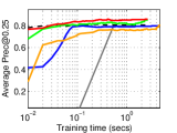
(a) KDD08

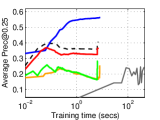
(b) Covtype

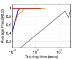
(c) Cod-RNA

Figure 4: A comparison of the proposed perceptron and SGD based methods with baseline methods (SVMPerf and 1PMB) on prec@0.25 maximization tasks.

References

- Agarwal [2011] S. Agarwal. The Infinite Push: A new support vector ranking algorithm that directly optimizes accuracy at the absolute top of the list. In 11th SIAM International Conference on Data Mining (SDM), pages 839–850, 2011.
- Boucheron et al. [2004] St phane Boucheron, G bor Lugosi, and Olivier Bousquet. Concentration inequalities. In Advanced Lectures in Machine Learning, pages 208–240. Springer, 2004.
- Boyd et al. [2012] Stephen Boyd, Corinna Cortes, Mehryar Mohri, and Ana Radovanovic. Accuracy at the top. In 26th Annual Conference on Neural Information Processing Systems (NIPS), pages 953–961, 2012.
- Burges et al. [2005] C. Burges, T. Shaked, E. Renshaw, A. Lazier, M. Deeds, N. Hamilton, and G. Hullender. Learning to rank using gradient descent. In 22nd International Conference on Machine Learning (ICML), pages 89–96, 2005.
- Calauzènes et al. [2012] Clément Calauzènes, Nicolas Usunier, and Patrick Gallinari. On the (Non-)existence of Convex, Calibrated Surrogate Losses for Ranking. In 26th Annual Conference on Neural Information Processing Systems (NIPS), 2012.
- Cao et al. [2007] Zhe Cao, Tao Qin, Tie-Yan Liu, Ming-Feng Tsai, and Hang Li. Learning to rank: from pairwise approach to listwise approach. In 24th International Conference on Machine learning (ICML), pages 129–136. ACM, 2007.
- Chakrabarti et al. [2008] Soumen Chakrabarti, Rajiv Khanna, Uma Sawant, and Chiru Bhattacharyya. Structured Learning for Non-Smooth Ranking Losses. In 14th ACM SIGKDD International Conference on Knowledge Discovery and Data Mining (KDD), 2008.
- Chaudhuri and Tewari [2014] Sougata Chaudhuri and Ambuj Tewari. Perceptron-like algorithms and generalization bounds for learning to rank. CoRR, abs/1405.0591, 2014.
- Chaudhuri and Tewari [2015] Sougata Chaudhuri and Ambuj Tewari. Online ranking with top-1 feedback. In 18th International Conference on Artificial Intelligence and Statistics (AISTATS), 2015.
- Clémençon and Vayatis [2007] Stéphan Clémençon and Nicolas Vayatis. Ranking the best instances. The Journal of Machine Learning Research, 8:2671–2699, 2007.
- Do et al. [2008] Chuong B. Do, Quoc Le, Choon Hui Teo, Olivier Chapelle, and Alex Smola. Tighter Bounds for Structured Estimation. In 22nd Annual Conference on Neural Information Processing Systems (NIPS), 2008.
- Freund et al. [2003] Y. Freund, R. Iyer, R. E. Schapire, and Y. Singer. An efficient boosting algorithm for combining preferences. Journal of Machine Learning Research, 4:933–969, 2003.
- Guruswami and Raghavendra [2009] Venkatesan Guruswami and Prasad Raghavendra. Hardness of learning halfspaces with noise. SIAM J. Comput., 39(2):742–765, 2009.
- Herbrich et al. [2000] R. Herbrich, T. Graepel, and K. Obermayer. Large margin rank boundaries for ordinal regression. In A. Smola, P. Bartlett, B. Schoelkopf, and D. Schuurmans, editors, Advances in Large Margin Classifiers, pages 115–132. MIT Press, 2000.
- Joachims [2002] T. Joachims. Optimizing search engines using clickthrough data. In 8th ACM SIGKDD International Conference on Knowledge Discovery and Data Mining (KDD), pages 133–142, 2002.
- Joachims [2005] Thorsten Joachims. A Support Vector Method for Multivariate Performance Measures. In 22nd International Conference on Machine Learning (ICML), 2005.
- Kar et al. [2014] Purushottam Kar, Harikrishna Narasimhan, and Prateek Jain. Online and stochastic gradient methods for non-decomposable loss functions. In 28th Annual Conference on Neural Information Processing Systems (NIPS), pages 694–702, 2014.
- Le and Smola [2007] Quoc V. Le and Alexander J. Smola. Direct optimization of ranking measures. arXiv preprint arXiv:0704.3359, 2007.
- Li et al. [2014] Nan Li, Rong Jin, and Zhi-Hua Zhou. Top rank optimization in linear time. In 28th Annual Conference on Neural Information Processing Systems (NIPS), pages 1502–1510, 2014.
- Minsky and Papert [1988] Marvin Lee Minsky and Seymour Papert. Perceptrons: An Introduction to Computational Geometry. MIT Press, 1988. ISBN 0262631113.
- Narasimhan and Agarwal [2013a] Harikrishna Narasimhan and Shivani Agarwal. A Structural SVM Based Approach for Optimizing Partial AUC. In 30th International Conference on Machine Learning (ICML), 2013a.
- Narasimhan and Agarwal [2013b] Harikrishna Narasimhan and Shivani Agarwal. : A New Support Vector Method for Optimizing Partial AUC Based on a Tight Convex Upper Bound. In 19th ACM SIGKDD Conference on Knowledge, Discovery and Data Mining (KDD), 2013b.
- Narasimhan et al. [2015] Harikrishna Narasimhan, Purushottam Kar, and Prateek Jain. Optimizing Non-decomposable Performance Measures: A Tale of Two Classes. In 32nd International Conference on Machine Learning (ICML), 2015.
- Novikoff [1962] A.B.J. Novikoff. On convergence proofs on perceptrons. In Proceedings of the Symposium on the Mathematical Theory of Automata, volume 12, pages 615–622, 1962.
- Prabhu and Varma [2014] Yashoteja Prabhu and Manik Varma. Fastxml: a fast, accurate and stable tree-classifier for extreme multi-label learning. In 20th ACM SIGKDD International Conference on Knowledge Discovery and Data Mining, KDD, pages 263–272, 2014.
- Rosenblatt [1958] Frank Rosenblatt. The perceptron: A probabilistic model for information storage and organization in the brain. Psychological Review, 65(6):386–408, 1958.
- Rudin [2009] C. Rudin. The p-norm push: A simple convex ranking algorithm that concentrates at the top of the list. Journal of Machine Learning Research, 10:2233–2271, 2009.
- Tsoumakas and Katakis [2007] Grigorios Tsoumakas and Ioannis Katakis. Multi-Label Classification: An Overview. International Journal of Data Warehousing and Mining, 3(3):1–13, 2007.
- Valizadegan et al. [2009] Hamed Valizadegan, Rong Jin, Ruofei Zhang, and Jianchang Mao. Learning to rank by optimizing NDCG measure. In 26th Annual Conference on Neural Information Processing Systems (NIPS), pages 1883–1891, 2009.
- Yue et al. [2007] Y. Yue, T. Finley, F. Radlinski, and T. Joachims. A support vector method for optimizing average precision. In 30th Annual International ACM SIGIR Conference on Research and Development in Information Retrieval (SIGIR), pages 271–278, 2007.
- Yun et al. [2014] Hyokun Yun, Parameswaran Raman, and S Vishwanathan. Ranking via robust binary classification. In 28th Annual Conference on Neural Information Processing Systems (NIPS), pages 2582–2590, 2014.
- Zhang [2002] Tong Zhang. Covering Number Bounds of Certain Regularized Linear Function Classes. Journal of Machine Learning Research, 2:527–550, 2002.