On the Reachability of Networked Systems

Abstract

In this paper, we study networks of discrete-time linear time-invariant subsystems. Our focus is on situations where subsystems are connected to each other through a time-invariant topology and where there exists a base-station whose aim is to control the subsystems into any desired destinations. However, the base-station can only communicate with some of the subsystems that we refer to as leaders. There are no direct links between the base-station and the rest of subsystems, known as followers, as they are only able to liaise among themselves and with some of the leaders.

The current paper formulates this framework as the well-known reachability problem for linear systems. Then to address this problem, we introduce notions of leader-reachability and base-reachability. We present algebraic conditions under which these notions hold. It turns out that if subsystems are represented by minimal state space representations, then base-reachability always holds. Hence, we focus on leader-reachability and investigate the corresponding conditions in detail. We further demonstrate that when the networked system parameters i.e. subsystems’ parameters and interconnection matrices, assume generic values then the whole network is both leader-reachable and base-reachable.

1 Introduction

Recent developments of enabling technologies such as communication systems, cheap computation equipment and sensor platforms have given great impetus to the creation of networked systems. Due to their large application in different branches of science and technology, these systems have attracted significant attention worldwide and researchers have studied networked systems from different perspectives (see e.g. [1], [2], [3], [4], [5], [6], [7]).

In this paper, we consider networks consisting of finite-dimensional linear time-invariant subsystems. We suppose that each subsystem in the network has discrete-time dynamics and the interconnection topology among subsystems is time-invariant. In the framework under study, there exists a base-station that can only send command signals to some of the subsystems with superior capabilities, known as leaders. The remainder of the subsystems referred to as followers can only accept input signals from some of the leaders and followers.

Here, we address a fundamental issue associated with the above framework namely the reachability. The concept of reachability is well-understood in the systems and control literature [8]. We adopt this concept to address the following question.

Under which conditions can the state of followers reach any desired values using the commands generated from the base-station?

We tackle this question by providing a mathematical model for the networked system under study. We introduce the notions of base-reachability and leader-reachability. Then we show that systems networked according to the model considered here are generically both base-reachable and leader-reachable. This means that when the parameters of the network i.e. parameter matrices of each subsystem as well as the interconnection topology, assume generic values, these properties hold. We also investigate some topologies that give rise to state matrices with symmetric or circulant structures.

The problem studied in this paper has some connections with the existing literature concerned with controllability of multi-agent systems. There exists a body of works in this area and among many, interested readers can refer to [9], [10], [11], [12], [13], [14], [10], [15] and references listed therein. These references studied the controllability problem for a group of single integrators connected through the nearest neighbourhood law. We comment on some of the works along this line in the next paragraph.

The controllability problem of multi-agent systems was proposed in [9] and the author formulated this problem as the controllability problem of linear systems, whose state matrices are induced from the graph Laplacian matrix. Necessary and sufficient algebraic conditions on the state matrices were given based on linear system tools. Under the same setup, a sufficient condition was derived in [16] where it was shown that the system is controllable if the null space of the leader set is a subset of the null space of the follower set. In [11], it was shown that a necessary and sufficient condition for controllability is not sharing any common eigenvalues between the Laplacian matrix of the follower set and the Laplacian matrix of the whole topology. However, it remains elusive on what exactly the graphical meaning of these rank conditions related to the Laplacian matrix is. This motivates several research activities on illuminating the controllability of multi-agent systems from a graph theoretic point of view. For example, a notion of anchored systems was introduced in [17], and it was shown that symmetry with respect to the anchored vertices makes the system uncontrollable. In [18], the authors characterized some necessary conditions for the controllability problem based on a new concept called leader-follower connectedness. While [18] was focused on the case of fixed topology, the corresponding controllability problem under switching topologies was investigated in [10], which employed some recent achievements in the switched systems literature. Later, the authors of [14] assumed the graph to be weighted with freely chosen entries. Under this setup, they proposed the notion of structural controllability for multi-agent systems. It turned out that this controllability notion, solely depends on the topology of the communication scheme; the multi-agent system is controllable if and only if the graph is connected. This result is later extended in [19] to the case where the dynamics of each subsystem are expressed by high order integrators rather than a single integrator. The authors of [20] examined the connection between the controllability of networks comprising single integrator subsystems and those consisting of subsystems with high order integrators.

The current paper has several contributions. Firstly, in contrast to the works described above, we relax the limitation imposed on subsystems dynamics by allowing subsystems to be general discrete-time linear time-invariant (DLTI) state space systems. Secondly, in most of the literature the followers are connected to one another by the nearest neighbourhood law. We relax this constraint here as well. Thirdly, as opposed to existing literature, we explicity examine the role of the base-station and its connections to the leaders.

The structure of this paper is as follows. In the next section, we formulate the problem under study. The main results of the paper are introduced in Section 3. Finally, Section 4 provides the concluding remarks and comments about future research directions.

2 Problem Formulation

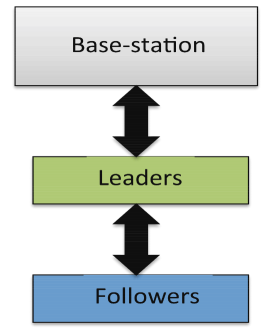
Figure 1: The connection structure between the base-station, leaders and follower

We assume that there exist $N$ linear subsystems which are connected together through linear coupling rules. Suppose that there exist $N_{l}$ subsystems with higher levels of computing and communicating powers that we refer to as leaders. The rest of the subsystems are called followers denoted by $N_{f}$. It is natural to assume that the number of leaders is strictly less than the number of followers i.e. $N_{f}>N_{l}$. The framework studied in this paper is depicted in Fig. 1.

Without loss of generality, we assume that the first $N_{f}$ subsystems are followers and the remaining $N-N_{f}$ subsystems act as leaders.

Suppose that the linear state space dynamics of the followers are expressed by a set of difference equations as

$$\begin{split}x^{i}_{t+1}&=A_{i}x^{i}_{t}+B_{i}v^{i}_{t},\\ w^{i}_{t}&=C_{i}x^{i}_{t},\;i=1,\dots,N_{f}.\end{split}$$ (1)

where $x^{i}_{t}\in\mathbb{R}^{n_{i}}$, $v^{i}_{t}\in\mathbb{R}^{m_{i}}$, $w^{i}_{t}\in\mathbb{R}^{p_{i}}$. We suppose that all $N$ subsystems are reachable and observable. The control command $v^{i}_{t}$ is constructed based on the following law

$$v^{i}_{t}=\sum_{j=1}^{N}L_{ij}w^{j}_{t}.$$ (2)

Remark 2.1.

Note that the control law (2) allows consideration of both centralized and distributed control schemes. If the control law (2) is implemented locally, then the control gains $L_{ij}$ corresponding to those subsystems which are not neighbors of $i$-th subsystem are assumed to be zero. This ensures that the summation $\sum_{j=1}^{N}{L_{ij}{w^{j}_{t}}}$ simplifies into a summation over the neighbor set of $i$-th subsystem. Hence, the control law (2) represents the topology of the network i.e. the matrices $L_{ij}$ represent which components of the state vector associated with the $j$-th subsystem are available to the local controller corresponding to the $i$-th subsystem. Thus, one can readily verify that the consensus law [21] can be regarded as a special case of the control strategy (2).

Let us also define the linear dynamics of each leader as

$$\begin{split}x^{i}_{t+1}&=A_{i}x^{i}_{t}+B_{i}u_{t},\\ w^{i}_{t}&=C_{i}x^{i}_{t},\>\>\>N_{f+1},\ldots,N,\end{split}$$ (3)

where $u_{t}\in\mathbb{R}^{m}$ is the control command generated from the base-station.

For our subsequent analysis it is convenient to define

$$\begin{split}\overline{A}_{f}&:=\mbox{\rm diag}\,(A_{1},\ldots,A_{N_{f}}),\\ \overline{B}_{f}&:=\mbox{\rm diag}\,(B_{1},\ldots,B_{N_{f}}),\\ C_{f}&:=\mbox{\rm diag}\,(C_{1},\ldots,C_{N_{f}}),\\ L&:=\begin{pmatrix}L_{11}&\ldots&{L_{1N}}\\ \vdots&\ddots&\vdots\\ L_{N_{f}1}&\ldots&L_{N_{f}N}\end{pmatrix}\in\mathbb{R}^{{m_{f}}\times\overline{p}},\\ x^{f}_{t}&:=\begin{pmatrix}x^{1}_{t}\\ \vdots\\ x^{N_{f}}_{t}\end{pmatrix}\in\mathbb{R}^{n_{f}},\\ v_{t}&:=\begin{pmatrix}v^{1}_{t}\\ \vdots\\ v^{N_{f}}_{t}\end{pmatrix}\in\mathbb{R}^{m_{f}},\\ w^{f}_{t}&:=\begin{pmatrix}w^{1}_{t}\\ \vdots\\ w^{N_{f}}_{t}\end{pmatrix}\in\mathbb{R}^{p_{f}}.\\ \end{split}$$ (4)

where $m_{f}=\sum_{i=1}^{N_{f}}m_{i}$, $p_{f}=\sum_{i=1}^{N_{f}}p_{i}$, $n_{f}=\sum_{i=1}^{N_{f}}n_{i}$, $\overline{p}=\sum_{i=1}^{N}p_{i}$.

We split the gain matrix $L$ as

$$L=\left(L_{ff}\>L_{lf}\right),$$

where $L_{ff}$ captures the first $p_{f}$ columns of $L$. This matrix captures the interconnection existing among followers only. Furthermore, $L_{lf}$ contains those columns of $L$ that are not contained in $L_{ff}$ and thereby exhibits the relation between followers and leaders.

In terms of the above quantities, the aggregated closed-loop system associated with the followers can be succinctly described via

$$\begin{split}x^{f}_{t+1}&=\underbrace{\left(\overline{A}_{f}+\overline{B}_{f}L_{ff}\mathcal{\overline{}}C_{f}\right)}_{A_{f}}x^{f}_{t}+\underbrace{\overline{B}_{f}L_{lf}C_{l}}_{B_{f}}x^{l}_{t},\\ w^{f}_{t}&=C_{f}x^{f}_{t}.\end{split}$$ (5)

We also record the aggregated dynamics for the leaders as

$$\begin{split}x^{l}_{t+1}&=A_{l}x^{l}_{t}+B_{l}u_{t},\\ w^{l}_{t}&=C_{l}x^{l}_{t},\end{split}$$ (6)

where

$$\begin{split}A_{l}&:=\mbox{\rm diag}\,(A_{N_{f}+1},\ldots,A_{N}),\\ B_{l}&:=\mbox{\rm diag}\,(B_{N_{f}+1},\ldots,B_{N}),\\ C_{l}&:=\mbox{\rm diag}\,(C_{N_{f}+1},\ldots,C_{N}),\\ x^{l}_{t}&:=\begin{pmatrix}x^{N_{f}+1}_{t}\\ \vdots\\ x^{N}_{t}\end{pmatrix}\in\mathbb{R}^{n_{l}},\\ w^{l}_{t}&:=\begin{pmatrix}w^{N_{f}+1}_{t}\\ \vdots\\ w^{N}_{t}\end{pmatrix}\in\mathbb{R}^{p_{l}},\end{split}$$ (7)

with dimensions $n_{l}=\sum_{i=N_{f}+1}^{N}n_{i}$ and $p_{l}=\sum_{i=N_{f}+1}^{N}p_{i}$.

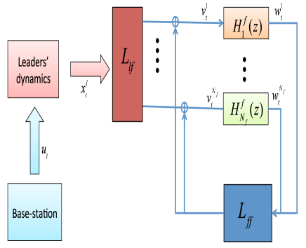
Figure 2: The dynamics of each follower are represented by $H^{f}_{i}(z)$, $i=1,\ldots,N_{f}$.

In this paper, our objective is to address the following question

Under which conditions can states of followers be steered into any desired values from any intial conditions, using the command signal $u_{t}$ and control law (2).

To this end, we first introduce Fig. 2 that provides a detailed pictorial description of the framework under study. It is clear that indeed there exist two levels of control in this framework i.e. from the base-station to leaders and from the leaders to followers.

3 Reachability of Networked Systems

We start this section by formally introducing definitions of reachability for each levels of control in Fig. 2. These definitions are adapted from the literature [22] for the purpose of the current paper.

Definition 3.1.

The follower dynamics (5) is said to be leader-reachable if and only if for any intial state $x^{f}_{t_{0}}\in\mathbb{R}^{n_{f}}$ and an arbirary final state $\bar{x}^{f}_{t_{f}}\in\mathbb{R}^{n_{f}}$, there exists $x^{l}_{t}$, $t\in[t_{0},t_{f}]$ such that $x^{f}_{t_{f}}=\bar{x}^{f}_{t_{f}}$.

Similarly for the dynamics (6), we state the following definition.

Definition 3.2.

The leader dynamics (6) is said to be base-reachable if and only if for any intial state $x^{l}_{t_{0}}\in\mathbb{R}^{n_{l}}$ and an arbirary final state $\bar{x}^{l}_{t_{f}}\in\mathbb{R}^{n_{l}}$, there exists $u_{t}$, $t\in[t_{0},t_{f}]$ such that $x^{l}_{t_{f}}=\bar{x}^{l}_{t_{f}}$.

The following lemma follows standard systems and control literature see e.g. [8].

Lemma 3.3.

The system (5)/(6) is leader-reachable/base-reachable if and only if the matrix $\mathcal{R}_{l}=\left(B_{f},\;A_{f}B_{f},\;\dots,\;A^{n_{f}-1}_{f}B_{f}\right)$/ $\mathcal{R}_{b}=\left(B_{l},\;A_{l}B_{l},\;\dots,\;A^{n_{l}-1}_{l}B_{l}\right)$ has full-row rank.

The above definitions enable us to introduce the following lemma.

Lemma 3.4.

Suppose the system (5) is leader-reachable and the system (6) is base-reachable. Then there exists $u_{t}$, $t\in[t_{0},t_{f}]$, such that for any arbirary final state $\bar{x}^{f}_{t_{f}}$, $x^{f}_{t_{f}}=\bar{x}^{f}_{t_{f}}$.

Proof.

Under the conditions in the lemma statement the reachable subspaces for the system (5) and (6) are equal to $\mathbb{R}^{n_{f}}$ and $\mathbb{R}^{n_{l}}$ respectively. Thus, one can always construct a proper input signal $u_{t}$ [22] to steer the states of the system (5) into any desired value. ∎

The result of Lemma 3.4 is illustrated further in the following example.

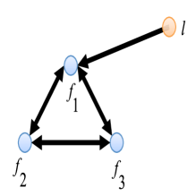
Figure 3: Followers are colored in blue and denoted by $f_{i}$ and the single leader is yellow indicated by $l$.

Example 3.5.

Consider a setup as shown in Fig. 3. For the sake of illustration, we suppose that all subsystems including followers and the leader have very simple dynamics described as follows

$$\bar{x}^{i}_{t+1}=0.2\bar{x}^{i}_{t}+\bar{v}^{i}_{t},\>\>i=1,\ldots,4,$$ (8)

with $\bar{v}^{i}_{t}=\sum_{j=1}^{4}\bar{L}_{ij}\bar{x}^{j}_{t}$, $i=1,2,3$ and $\bar{v}^{4}_{t}=u_{t}$.

Given the dynamics (8), all subsystems are reachable. We let the parameters $\bar{L}_{21}=\bar{L}_{31}=1$, $\bar{L}_{21}=\bar{L}_{23}=2$ and $\bar{L}_{31}=\bar{L}_{32}=3$. Then it is easy to verify that the follower dynamics are

$$\begin{pmatrix}\bar{x}^{1}_{t+1}\\ \bar{x}^{2}_{t+1}\\ \bar{x}^{3}_{t+1}\end{pmatrix}=\underbrace{\begin{pmatrix}0.2&1&1\\ 2&0.2&2\\ 3&3&0.2\end{pmatrix}}_{A_{f}}\begin{pmatrix}\bar{x}^{1}_{t}\\ \bar{x}^{2}_{t}\\ \bar{x}^{3}_{t}\end{pmatrix}+\underbrace{\begin{pmatrix}1\\ 0\\ 0\end{pmatrix}}_{B_{f}}\bar{x}^{4}_{t+1}.$$ (9)

It can be checked that this system is base-reachable. Given the dynamics (8), one can conclude that the states of the system (9) can be driven into any desired point in the space using the input command $u_{t}$.

3.1 Leader Reachability

In the previous subsection, we introduced the notions of leader-reachability and base-reachability. It is worthwhile to investigate these notions when networked systems attain special interconnection structures. This is because in different applications, subsystems may be linked to each other in particular forms see e.g. [2], [23], [24]. Thus, in this subsection, we aim to explore networked systems with special structures.

One should note that when the pairs $A_{i},B_{i}$ are reachable, the base-reachability of the system (6) becomes immediate. However, it still remains a nontrivial task to explore the concept of leader-reachability for the system (5). In this subsection we study this notion in more detail.

The analysis of leader-reachability for the system (5) is very intricate in general. This is because the state matrix $A_{f}$ has an involved structure. Furthermore, networks with special coupling structures appear in many applications, such as cyclic pursuit [25]; shortening flows in image processing [26] or the discretization of partial differential equations [24]. Thus, in order to provide some rigorous results we study the notion of leader-reachability when the state matrix attains some particular structures. Here, we consider two scenarios namely symmetric $A_{f}$ and circulant $A_{f}$.

3.1.1 Symmetric $A_{f}$

Several interconnection topologies can lead to a symmetric $A_{f}$ matrix. For instance, consider a scenario where a set of scalar subsystems are connected to each other based on the consensus law [2].

Theorem 3.6.

Suppose that the matrix $A_{f}$ is symmetric. Let $\lambda_{i}$ and $\nu_{i}$, $\forall i\in\{1,2,\ldots,n_{f}\}$, denote eigenvalues and the corresponding eigenvectors of $A_{f}$ and $B_{f}=\left(b_{f}^{1},\;\ldots,\;b_{f}^{m_{f}}\right)$. Then the dynamics (5) is leader-reachable if $\lambda_{i}\neq\lambda_{j}$ and $\nu^{T}_{i}b_{f}^{j}\neq 0$ $\forall i,j$.

Proof.

In this case, the matrix $A_{f}$ can be written as $Q\Lambda Q^{\top}$ where $Q$ is an orthonormal matrix comprised of $\nu_{i}$ and $\Lambda$ is a diagonal matrix containing eigenvalues of $A_{f}$. It is easy to see that

$$\begin{split}\mathcal{R}_{l}&=\left(B_{f},\;Q\Lambda Q^{\top}B_{f},\ldots,Q\Lambda^{n_{f}-1}Q^{\top}B_{f}\right)\\ &=Q\underbrace{\left(Q^{\top}B_{f},\;\Lambda Q^{\top}B_{f},\ldots,\Lambda^{n_{f}-1}Q^{\top}B_{f}\right).}_{\overline{\mathcal{R}}_{l}}\ \end{split}$$

The matrix $Q$ has full rank. Thus, the rank of $\mathcal{R}_{l}$ is determined by $\overline{\mathcal{R}}_{l}$ that is expressed as

$$\begin{split}&\left(\begin{pmatrix}\nu_{1}^{\top}\\ \vdots\\ \nu_{n_{f}}^{\top}\end{pmatrix}\begin{pmatrix}b_{f}^{1}&\ldots&b_{f}^{m_{f}}\end{pmatrix},\;\begin{pmatrix}\lambda_{1}&&\\ &\ddots&\\ &&\lambda_{n_{f}}\end{pmatrix}\begin{pmatrix}\nu_{1}^{\top}\\ \vdots\\ \nu_{n_{f}}^{\top}\end{pmatrix}\right.\\ &\left.\begin{pmatrix}b_{f}^{1}&\ldots&b_{f}^{m_{f}}\end{pmatrix},\;\ldots,\begin{pmatrix}\lambda_{1}&&\\ &\ddots&\\ &&\lambda_{n_{f}}\end{pmatrix}^{n_{f}-1}\begin{pmatrix}\nu_{1}^{\top}\\ \vdots\\ \nu_{n_{f}}^{\top}\end{pmatrix}\right.\\ &\left.\begin{pmatrix}b_{f}^{1}&\ldots&b_{f}^{m_{f}}\end{pmatrix}\right.\Bigg{)}.\end{split}$$

By appealing to the theorem assumptions and the fact that $\nu_{i}^{\top}\nu_{j}\neq 0$ $\forall i\neq j$, the result immediately follows. ∎

3.1.2 Circulant $A_{f}$

In this subsection, we study the situation where the matrix $A_{f}$ has circulant structure. This situation may happen naturally when the interconnection topology is a circulant graph see e.g [23]. It is worthwhile noting that networked systems with circulant topology arise in different applications such as quantum communication [27] and complex memory management [28].

The following example illustrates a situation where the matrix $A_{f}$ acquires a circulant structure.

Example 3.7.

Let us consider a network consisting of four identical single-output-single-output (SISO) subsystems. We suppose the dynamics for each subsystem are expressed as

$$\begin{split}\hat{x}^{i}_{t+1}&=a\hat{x}^{i}_{t}+b\hat{v}^{i}_{t},\\ \hat{w}^{i}_{t}&=\hat{x}^{i}_{t},\;i=1,\dots,4.\end{split}$$

with $|a|<1$. $\hat{v}^{i}_{t}=\sum_{j=1}^{4}\hat{L}_{ij}\hat{x}^{j}_{t}$, $i=1,2,3$ and $\hat{v}^{4}_{t}=u_{t}$.

As shown in Fig. 4, the interconnection parameters i.e. $\hat{L}_{ij}$ are set as $\hat{L}_{12}=\hat{L}_{23}=\alpha_{1}$, $\hat{L}_{13}=\hat{L}_{21}=\hat{L}_{32}=\alpha_{2}$, $\hat{L}_{32}=\alpha_{3}$, $\hat{L}_{14}=b$ and $\hat{L}_{24}=\hat{L}_{34}=0$. Then it is easy to verify that $A_{f}=\begin{pmatrix}a&\alpha_{1}&\alpha_{2}\\ \alpha_{2}&a&\alpha_{1}\\ \alpha_{3}&\alpha_{2}&a\end{pmatrix}$ and $B_{f}=\begin{pmatrix}b\\ 0\\ 0\end{pmatrix}$. We set parameter of dynamics and topology to be $a=0.2$, $b=\alpha_{1}=\alpha_{3}=1$ and $\alpha_{2}=0.5$. Then it can be checked that the whole network depicted in Fig. 4 is reachable.

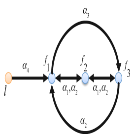
Figure 4: Followers are colored in blue and denoted by $f_{i}$ and the sole leader is yellow indicated by $l$. The weighting coefficients on connecting links are represented by $\alpha_{i}$.

As mentioned earlier, the matrix $A_{f}$ in the above example has a particular form known as circulant. Thus, we now investigate in more detail a scenario where the matrix $A_{f}$ has circulant structure i.e. is of the form

$$\begin{split}A_{f}&=\rm{Circ}(\alpha_{0},...,\alpha_{n_{f}-1})\\ &=\begin{pmatrix}\alpha_{0}&\alpha_{1}&\cdots&\alpha_{n_{f}-2}&\alpha_{n_{f}-1}\\ \alpha_{n_{f}-1}&\alpha_{0}&\alpha_{1}&\cdots&\alpha_{n_{f}-2}\\ \vdots&\ddots&\ddots&\ddots&\vdots\\ \alpha_{2}&\cdots&\alpha_{n_{f}-1}&\alpha_{0}&\alpha_{1}\\ \alpha_{1}&\alpha_{2}&\cdots&\alpha_{n_{f}-1}&\alpha_{0}\end{pmatrix}.\end{split}$$

It is well-known that circulant matrices [29] are diagonalizable by the Fourier matrix

$$\begin{split}\Phi&=\frac{1}{\sqrt{n_{f}}}\begin{pmatrix}1&1&1&\ldots&1\\ 1&\omega&\omega^{2}&\ldots&\omega^{n_{f}-1}\\ 1&\omega^{2}&\omega^{4}&\ldots&\omega^{2n_{f}-2}\\ \vdots&&&&\\ 1&\omega^{n_{f}-1}&\omega^{2n_{f}-2}&\ldots&\omega^{(n_{f}-1)^{2}}\end{pmatrix}\text{ ,}\\ &=\frac{1}{\sqrt{n_{f}}}\begin{pmatrix}\phi_{1}\\ \phi_{2}\\ \vdots\\ \phi_{n_{f}}\end{pmatrix}\end{split}$$

where $\omega=e^{2\pi j/{n_{f}}}$ denotes a primitive $n_{f}-$th root of unit and $\phi_{i}$ denote rows of $\Phi$. Note, that $\Phi$ is both a unitary and a symmetric matrix. It is then easily seen that any circulant matrix $L$ has the form $A_{f}=\Phi\mbox{\rm diag}\,(p_{L}(1),p_{L}(\omega),\ldots,p_{L}(\omega^{n_{f}-1}))\Phi^{*},$ $=\Phi\Gamma\Phi^{*}$ where $p_{L}(z):=\sum_{k=0}^{n_{f}-1}c_{k}z^{k-1}.$ As a consequence of the preceding analysis we obtain the following result.

Theorem 3.8.

Suppose that the matrix $A_{f}$ is circulant and $B_{f}=\left(b_{f}^{1},\;\ldots,\;b_{f}^{m_{f}}\right)$. Then the dynamics (5) is leader-reachable if $\phi^{\top}_{i}b_{f}^{j}\neq 0$, $\forall i,j$.

Proof.

From the above analysis, one can write

$$\begin{split}\mathcal{R}_{l}&=\left(B_{f},\;\Phi\Gamma\Phi^{*}B_{f},\ldots,\Phi\Gamma^{n_{f}-1}\Phi^{*}B_{f}\right)\\ &=\Phi\underbrace{\left(\Phi^{*}B_{f},\;\Gamma\Phi^{*}B_{f},\ldots,\Gamma^{n_{f}-1}\Phi^{*}B_{f}\right)}_{\underline{\mathcal{R}}_{l}}\ \end{split}$$

Now by using the same argument as in the proof of Theorem 3.6 the result immediately follows. ∎

3.2 Generic Reachability

The previous subsection examined the leader-reachability and base-reachability notions for special network structures. In this subsection, we show that these properties hold in almost all cases. To this end, we first need to define the parameter space $\Theta$ as

$$\begin{split}\Theta=&\{\mbox{\rm vec}\,\left(A_{1},\ldots,A_{N}\right),\mbox{\rm vec}\,\left(B_{1},\ldots,B_{N}\right),\\ &\mbox{\rm vec}\,\left(C_{1},\ldots,C_{N}\right),\mbox{\rm vec}\,(L)\}.\end{split}$$ (10)

Then we recall the notion of generic set from [30]. A subset of the parameter space $\Theta$ is said to be generic if it is an open and dense in $\Theta$. We now use this notion to introduce the next results.

Theorem 3.9.

The systems (5) and (6) are leader-reachable and base-reachable on a generic subset of the parameter space $\Theta$.

Proof.

First, one can easily find a set of matrices $A_{i}$,$B_{i}$, etc., such that the associated matrix $\mathcal{R}_{l}$ attains full- row rank. Second, let $\sigma_{i}$ $i=1,\ldots,n_{f}m_{f}$ denote the columns of $\mathcal{R}_{l}$ defined in Lemma 3.3. Then note that the system (5) is not reachable if and only if

$$\det\{\Gamma\}=0,$$ (11)

where $\Gamma\in\mathbb{R}^{n_{f}\times n_{f}}$ and the columns of $\Gamma$ are constructed by selecting any $n_{f}$ choice of $\sigma_{i}$. Then the set of zeros of (11) defines a proper algebraic set. Therefore, its complement, which is associated with all reachable systems, is the complement of a proper algebraic set and hence is open and dense in the parameter space. The latter is equivalent to the statement of the theorem. Finally, note that those parts of the theorem statement asssociated with the system (6) become trivial in the light of [31] pages 44-45. ∎

The preceding result roughly suggests that for almost all choices of parameter matrices $A_{i}$, $B_{i}$ and etc., there exists a $u_{t}$ that can steer the follower and leader states to desired values.

4 Conclusion and Future Works

We examined the reachability problem for networked systems. It was assumed that all subsystems are expressed by discrete linear time-invariant state space models.

We considered the network topology to be time-invariant. We addressed a hierarchical framework where there exists a base-station at the highest level; superior subsystems (leaders) are at an intermediate level and the rest of subsystems (followers) stay at the final stage. The followers are only able to communicate with each other and with leaders only. We introduced notions of leader-reachability and base-reachability. We explored situations under which the algebraic criteria associated with these notions are satisfied. It turned out that the reachability of leaders is enough for fulfilling base-reachability. We then studied leader-reachability and provided algebraic conditions for this property to hold. We examined different topologies such as those that give rise to symmetric and circulant state matrices. We further demonstrated that when the system parameters assume generic values, the whole network is reachable.

There are several interesting problems that still remain open. The scenarios discussed in this paper only cover certain classes of linear networked systems. It would be of interest to provide a result that includes more general instances. Another problem involves studying reachability for a scenario where interconnection matrices assume only zero and free entries. This problem is highly related with the structural controllability problem studied in the literature [32]. Another interesting issue is associated with control energy of the whole networked system. In particular, we are interested in designing topologies such that reachability is preserved but the deployed control energy remains within some given boundaries as well.

References

- [1] B. Sinopoli, C. Sharp, L. Schenato, S. Schaffert, S. Sastry, Distributed control applications within sensor networks, Proceedings of the IEEE 91 (8) (2003) 1235–1246.
- [2] R. Olfati-Saber, R. M. Murray, Distributed cooperative control of multiple vehicle formations using structural potential functions, in: Proc the IFAC World Congress, 2002, pp. 346–352.
- [3] H. G. Tanner, A. Jadbabaie, G. J. Pappas, Stable flocking of mobile agents part I: dynamic topology, in: Proc the IEEE Conference on Decision and Control, 2003, pp. 2016–2021.
- [4] R. Olfati-Saber, J. A. Fax, R. M. Murray, Consensus and cooperation in networked multi-agent systems, Proceedings of the IEEE 95 (1) (2007) 215–233.
- [5] A. G. Dankers, System identification in dynamic networks, Ph.D. thesis, TU Delft, Delft University of Technology (2014).
- [6] P. J. Hespanha, P. Naghshtabrizi, Y. Xu, A survey of recent results in networked control systems, IEEE Proceedings 95 (1) (2007) 138–162.
- [7] M. Zamani, U. Helmke, B. D. O. Anderson, Zeros of networked systems with time-invariant interconnections, submitted for publication (http://arxiv.org/abs/1408.6889).
- [8] T. Kailath, Linear Systems, Prentice-Hall, New Jersey, 1980.
- [9] H. G. Tanner, On the controllability of nearest neighbor interconnections, in: Proc the IEEE Conference on Decision and Control, Vol. 3, 2004, pp. 2467–2472.
- [10] Z. Ji, H. Lin, T. H. Lee, Controllability of multi-agent systems with switching topology., in: Proc of the IEEE conference on Robotics, Automation and Mechatronics, 2008, pp. 421–426.
- [11] M. Ji, M. Egerstedt, A graph-theoretic characterization of controllability for multi-agent systems, in: Proc the American Control Conference, 2007, pp. 4588–4593.
- [12] A. Rahmani, M. Ji, M. Mesbahi, M. Egerstedt, Controllability of multi-agent systems from a graph-theoretic perspective, SIAM Journal on Control and Optimization 48 (1) (2009) 162–186.
- [13] Y.-Y. Liu, J.-J. Slotine, A.-L. Barabási, Controllability of complex networks, Nature 473 (7346) (2011) 167–173.
- [14] M. Zamani, H. Lin, Structural controllability of multi-agent systems, in: Proc the American Control Conference, 2009, pp. 5743–5748.
- [15] S. Martini, M. Egerstedt, A. Bicchi, Controllability analysis of multi-agent systems using relaxed equitable partitions, International Journal of Systems, Control and Communications 2 (1) (2010) 100–121.
- [16] M. Ji, A. Muhammad, M. Egerstedt, Leader-based multi-agent coordination: controllability and optimal control, in: Proc the American Control Conference, 2006.
- [17] A. Rahmani, M. Mesbahi, On the controlled agreement problem, in: Proc the American Control Conference, 2006, 2006.
- [18] Z. Ji, H. Lin, T. H. Lee, A graph theory based characterization of controllability for multi-agent systems with fixed topology, in: Proc the IEEE Conference on Decision and Control, 2008, pp. 5262–5267.
- [19] A. Partovi, L. Hai, J. Zhijian, Structural controllability of high order dynamic multi-agent systems, in: Proc the IEEE Conference on Robotics, Automation and Mechatronics, 2010.
- [20] L. Wang, F. Jiang, G. Xie, Z. Ji, Controllability of multi-agent systems based on agreement protocols, Science in China Series F: Information Sciences 52 (11) (2009) 2074–2088.
- [21] J. A. Fax, R. M. Murray, Information flow and cooperative control of vehicle formations, IEEE Transactions on Automatic Control 49 (9) (2004) 1465–1476.
- [22] J. P. Hespanha, Linear Systems Theory, Princton University Press, 2009.
- [23] M. Nabi-Abdolyousefi, M. Mesbahi, On the controllability properties of circulant networks, IEEE Transactions on Automatic Control 58 (12) (2013) 3179–3184.
- [24] R. W. Brockett, J. L. Willems, Discretized partial differential equations: Examples of control systems defined on modules, Automatica 10 (5) (1974) 507–515.
- [25] J. A. Marshall, M. E. Broucke, B. A. Francis, Formations of vehicles in cyclic pursuit, IEEE Transactions on Automatic Control 49 (11) (2004) 1963–1974.
- [26] M. A. Bruckstein, G. Sapiro, D. Shaked, Evolutions of planar polygons., International Journal of Pattern Recognition and Artificial Intelligence 9 (6) (1995) 991–1014.
- [27] A. Ilić, M. Bašić, New results on the energy of integral circulant graphs, Applied Mathematics and Computation 218 (7) (2011) 3470 – 3482.
- [28] C. K. Wong, D. Coppersmith, A combinatorial problem relatedto multimodule memory organizations, Journal of the ACM 21 (3) (1974) 392–402.
- [29] P. J. Davis, Circulant matrices, John Wiley and Sons. New York, 1979.
- [30] B. D. Anderson, M. Deistler, E. Felsenstein, B. Funovits, L. Koelbl, M. Zamani, Multivariate AR systems and mixed frequency data: G-identifiability and estimation, Econometric Theory (2015) 1–34.
- [31] W. M. Wonham, Linear Multivariable Control: a Geometric Approach, Springer-Verlag, New York, 1979.
- [32] C.-T. Lin, Structural controllability, IEEE Transactions on Automatic Control 19 (3) (1974) 201–208.