Solution space structure of random constraint satisfaction problems with growing domains

Abstract

In this paper we study the solution space structure of model RB, a standard prototype of Constraint Satisfaction Problem (CSPs) with growing domains. Using rigorous the first and the second moment method, we show that in the solvable phase close to the satisfiability transition, solutions are clustered into exponential number of well-separated clusters, with each cluster contains sub-exponential number of solutions. As a consequence, the system has a clustering (dynamical) transition but no condensation transition. This picture of phase diagram is different from other classic random CSPs with fixed domain size, such as random $K$-Satisfiability (K-SAT) and graph coloring problems, where condensation transition exists and is distinct from satisfiability transition. Our result verifies some non-rigorous results obtained using cavity method from spin glass theory.

I Introduction

Constraint satisfaction problems are defined as a set of discrete variables whose assignments must satisfy a collection of constraints. A CSP instance is said to be satisfiable if there exists a solution, i.e. an assignment to all variables that satisfies all the constraints. The core question to CSPs is to decide whether a given instance is satisfiable. CSPs have been studied extensively in mathematics and computer science, and play an important role in the computational complexity theory. Most of the interesting CSPs, such as boolean K-satisfiability problems and graph coloring problems, are belong to class of NP-complete: in the worst case the time required to decide whether there exists a solution increases very quickly as the size of the CSP grows.

In recent years, there are many interests on the average case complexity of CSPs, which study the computational complexity of random ensembles of CSPs. It also has drawn considerable attention in statistical physics, especially in the field of spin glasses. From a statistical physics’ viewpoint, finding solutions of CSPs amounts to find the ground-state configurations of spin glasses at zero temperature, where the energy represents the number of violated constraints. Most interesting CSPs also display a spin glass behavior at thermodynamic limit (with number of variables $N\to\infty$, and number of constraints $M\to\infty$), and encounters set of phase transitions when constraint density $c=\frac{M}{N}$ increases. The first transition that caught lots of interests is the satisfiability transition $c_{s}$ Kirkpatrick, and Selman ; Monasson, and Zecchina ; Mézard, Parisi, and Zecchina where the probability of a random instance being satisfiable changes sharply from $1$ to $0$. In the satisfiable phase (the parameter regime that w.h.p. random instances are solvable), studies using cavity method Mézard and Parisi (2002); Mézard and Zecchina (2002) from spin glass theory tell us that the solution space of CSPs are highly structured: with $c$ increasing, system undergoes clustering transition, condensation transition and finally satisfiability transition Krzakala et al. (2007); Montanari, Tersenghi, and Semerjian ; color . All of these transitions are connected to the fact that solutions are clustered into clusters. The clustering phenomenon is believed to effect performance of solution-finding algorithms and to be responsible for the hardness of CSPsKrzakala et al. (2007).

Besides heuristic analysis using cavity method, rigorous mathematical studies have also made lots of progress on the satisfiability transitions and clustering of solutions in CSPs: some CSP models have been proved to have satisfiability transition such as K-XORSAT and K-SAT with growing clause length; some CSP models have been proven to have a clustering phase, such as K-SAT ($K\geq 8$), K-coloring and hypergraph 2-coloring Mézard, Mora, and Zecchina ; Achlioptas, coja-oghlan, and Tersenghi ; Achlioptas, and coja-oghlan . Hypergraph 2-coloring has been proven to have condensation phase in coja-oghlan, and Zdeborova .

In this paper we study model RB Xu, and Li , a prototype CSP model with growing domains that is revised from the famous CSP Model B Smith, and Dyer . The main difference between model RB and classic CSPs like satisfiability problems is that number of states (we called domain size here) one variable can take is an increasing function of number of variables. This is probably one of the reason that makes the satisfiability threshold rigorously solvable Xu, and Li , and the clustering of solutions also provable as we will show in the main text of this paper. It has been shown that random instances of model RB are hard to solve close to satisfiability transition Xu, and Li ; Xu, Boussemart, Hemery, and Lecoutre ; Liu, Lin and Wang ; Zhao, Zhang, Zheng, and Xu , and benchmarks based on model RB (more information on http://www.nlsde.buaa.edu.cn/~kexu/) have been widely used in algorithmic research and in various kinds of algorithm competitions (e.g., CSP, SAT and MaxSAT) in recent years. Model RB has also been used or investigated in many different fields of computer science. Hardness of model RB makes the relation between its solution space structure and its hardness an interesting problem.

Using cavity method, it has been shown that Zhao, Zhang, Zheng, and Xu replica symmetry solution is always stable in the satisfiable phase, which suggests that condensation transition does not exist in this problem. Here we use rigorous methods, namely the first and the second moment method dimitris and moore ; Achlioptas, coja-oghlan, and Tersenghi , to show that in the satisfiable phase close to the satisfiability transition, solutions are always clustered into exponential number of clusters, and each cluster contains sub-exponential number of solutions. So we are showing rigorously that the system has no condensation transition.

The main contributions of this paper are twofold:

• From mathematical point of view, we give a rigorous analysis on the geometry of solution clusters in model RB problems.

• From statistical physics point of view, we show that there is no condensation transition in this this problem. Thus as a consequence, replica symmetry results including Bethe entropy and marginals given by cavity method and associated Belief Propagation algorithm, should be asymptotically exact.

The rest of the paper is organized as follows. Section II includes definitions of model RB and brief descriptions on previously obtained results on phase transitions of model RB. Sec. III contains our main results which include rigorous analysis on clustering of solutions, number and diameter of clusters. We conclude this work in Sec. IV.

II Model RB and phase transitions

Random CSP model provides a relatively “unbiased” samples for testing algorithms, helping design better algorithms and heuristics, provides insight into complexity theory. The standard random models (such as model B) suffer from (trivial) insolubility as problem size increases, then models with varying scales of parameters was proposed to overcome this deficiency Lecoutre and (2009); smith2001 ; frize ; fan2011 ; fan2012 . Model RB is one of them, who has growing domain size. It is worth mentioning that CSPs with growing domains can describe many practical problems better, for example N-queens problem, Latin square problem, sudoku, and Golomb ruler problem.

Here is the definition of model RB. An instance of model RB contains $N$ variables, each of which takes values from its domain $D=\{1,2,\cdots,d_{N}\}$, with $d_{N}=N^{\alpha}$. Note that the domain size $|D|$ is growing polynomially with system size $N$, and this is the main difference between model RB and classic CSPs like K-SAT problems. There are $M=rN\ln N$ constrains in one instance, each constraint involves $k$ ($k\geq 2$) different variables that chosen randomly and uniformly from all variables. Total number of assignments of variables involved by a constraint is $d_{N}^{k}$. For a constraint $a$ we pick up randomly $pd_{N}^{k}$ different assignments from totally $d_{N}^{k}$ assignments to form an incompatible-set $Q_{a}$. In other words constraint $a$ is satisfiable by the assignment $\left\{\sigma_{a}\right\}=\left\{\sigma_{a1},\sigma_{a2},...,\sigma_{ak}\right\}$ if $\left\{\sigma_{a}\right\}\not\in Q_{a}$.

So given parameters ($N,k,r,\alpha,p$), an instance of model RB is generated as follows

1. Select (with repetition) $rN\ln N$ random constraints, each of which is formed by selecting (without repetition) randomly $k$ variables.

2. For each constraint, we form an incompatible-set by uniformly select (without repetition) $pN^{\alpha k}$ elements of $D^{k}$.

Note that here we consider

$$p<1-\frac{1}{k},$$ (1)

in order to exclude too few configurations in each constraint, and to facilitate the derivation.

Given an instance of model RB, the task is to find a solution, i.e. an assignment that satisfies all the constraints simultaneously. It is easy to see that total number of configurations is $N^{\alpha N}$, each of which has probability $(1-p)^{rN\ln N}$ to satisfy all the constraints. If we use $X$ to denote number of solutions in one instance, the expectation of it over all possible instances can be written as

$$\mathbb{E}(X)=N^{\alpha N}(1-p)^{rN\ln N}.$$ (2)

Let

$$r^{*}=-\frac{\alpha}{\ln(1-p)},$$ (3)

we can see that with $r>r^{*}$, expectation of number of solutions is nearly $0$ for large $N$. Using Markov’s inequality

$$P(X>0)\leq\mathbb{E}(X),$$

we know that $\mathbb{E}(X)$ gives an upper bound for probability of a formula being satisfiable. So for sure with $r>r^{*}$ w.h.p. there is no solution in an instance of model RB. With $r<r^{*}$, though expectation of number of solutions is larger than $0$, these solutions may distributed non-uniformly, that is some instances may contain exponentially many solutions while in other instances there could be no solution at all.

Fortunately in model RB it has been shown Xu, and Li that $\mathbb{E}(x)$ is square root of expectation of the second moment of number of solutions with $r<r^{*}$, hence solutions are indeed distributed uniformly. More precisely, with $N\to\infty$, using Cauchy’s inequality, with $r<r^{*}$ we have

$$P(X>0)\geq\frac{E^{2}(X)}{E(X^{2})}\rightarrow 1,$$ (4)

In other words, the satisfiability transition happens at $r^{*}$:

$$\lim_{n\rightarrow\infty}{\text{Pr}(X>0)}=1\ \text{when}\ r<r^{*}$$

$$\lim_{n\rightarrow\infty}{\text{Pr}(X>0)}=0\ \text{when}\ r>r^{*}.$$

However even in the satisfiable phase close to the satisfiability transition, where we almost sure there are solutions, it is still difficult to find a solution in an random instance. Actually many efforts have been devoted to designing efficient algorithms that work in this regime. So far, our understanding on this algorithmically hardness is based on the clustering of solutions in the satisfiable regime close to transition. In statistical physics, the methods that we can use to describe the solutions space structure are borrowed from cavity method in spin glass theory. From statistical physics point of view, CSP problems are nothing but spin glass models at zero temperature, with energy of the system defined as number of violated constraints in CSPs. Thus finding a solution is equivalent to finding a configuration $\left\{\sigma\right\}=\left\{\sigma_{i}|i=1,...,N\right\}$ that has zero energy. More precisely one can define a Gibbs measure

$$P(\left\{\sigma\right\})=\frac{1}{Z}e^{\beta\sum_{a=1}^{M}E_{a}(\left\{\sigma_{a}\right\})},$$

where $Z$ is partition function, $E_{a}(\left\{\sigma_{a}\right\})$ is $0$ if ${\left\{\sigma_{a}\right\}\not\in Q_{a}}$ and is $1$ otherwise. By taking $\beta\to\infty$, and using e.g. cavity method, one can study properties of this Gibbs distribution reflecting the structure of solutions space Krzakala et al. (2007), such as whether ground-state energy is $0$, whether Gibbs distribution is extremal, whether replica symmetry is broken etc. The previous study Krzakala et al. (2007); Montanari, Tersenghi, and Semerjian ; color have shown that the similar picture of structure of configuration space and phase transitions exist in lots of interesting constraint satisfaction problems: when number of constraints is small, replica symmetry holds and Gibbs measure is extremal. With number of constraints (or edges in the graph) increasing, system undergoes clustering, condensation and satisfiability transitions respectively. At the clustering transition (also called dynamical transition), set of solutions begins to split into exponentially number of pure states, and replica symmetry holds in each pure state. At the condensation transition, size of clusters becomes inhomogeneous such that a finite number of clusters contains almost all the solutions. If the number of constraints keeps increasing and beyond satisfiability transition, neither cluster nor solution exists any more. Note that in some CSPs like K-SAT problem with $K=3$ and some combinatorial optimization problems like independent set problem vc1 ; vc2 with low average degree, clustering transition and condensation transition are identical. While for some other problems like K-SAT problem with $K\geq 4$ and graph coloring problem, condensation transition is distinct from clustering transition, and there is a stable one step replica symmetry breaking (1RSB) phase.

Studies based on replica symmetry cavity method and its associated Belief Propagation equations have been applied to model RB in Zhao, Zhang, Zheng, and Xu , and Bethe entropy $S_{\text{Bethe}}$ (leading order of logarithm of number of solutions) has been calculated on single instances. There are two interesting observations in Zhao, Zhang, Zheng, and Xu . First, BP equations always converge on single instances when energy reported by BP is zero. It means that in the satisfiable phase BP is always marginally stable, indicating that replica symmetry solution is always locally stable in satisfiable phase; Second, Bethe entropy agrees very well with first moment estimate of entropy (annealed entropy) $S_{\text{Bethe}}=\ln\mathbb{E}(X)$. These two phenomenons suggest that Belief Propagation algorithm may give a asymptotically correct marginal and free energy, and condensation transition does not exist.

III solution space structure of model RB

Heuristic analysis on solution space structure using cavity method and replica symmetry breaking are based on the concept of pure state, with assumptions of extremal Gibbs measure and exponential growth of both number of clusters and number of solutions in each cluster. Following Achlioptas, and Ricci-Tersenghi , in this paper we use a more concrete definition of cluster using the Hamming distance. Let us use $\mathcal{S}$ to denote set of all solutions in an instance. The Hamming distance between two arbitrary solutions $x,y\in\mathcal{S}$, noted $d(x,y)$, is the number of configurations taking different values in $x,y$. We define diameter of an set of solution $X\subseteq\mathcal{S}$ as the maximum Hamming distance between any two elements of $X$. The distance between two sets $X,Y\subseteq\mathcal{S}$, is the minimum Hamming distance between any $x\in X$ and any $y\in Y$. We define cluster as a connected component of $\mathcal{S}$, where every $x,y\in\mathcal{S}$ are considered adjacent if they are at Hamming distance 1 (or an finite integer $q$, it does not affect the conclusion). We further define region as union of some non-empty clusters.

III.1 clustering of solutions

Our analysis is based on the number of solution pairs $Z(x)$ at Hamming distance $Nx$, with $0<x<1$. Again as it is hard to compute $Z(x)$ exactly, we turn to the expectation of $Z(x)$. As shown in Xu, and Li , the number of assignment pairs at distance $Nx$ is equal to

$$t(x)=N^{\alpha N}\binom{N}{Nx}(N^{\alpha}-1)^{Nx};$$

probability of a pair of assignments being two solutions is written as

$$q(x)=\{(1-p)^{2}+p(1-p)[(1-x)^{k}+g(x)]\}^{rN\ln{N}},$$

where

$$g(x)=\frac{-k(k-1)x(1-x)^{k-1}}{2N}.$$

So the expectation of $Z(x)$, denoted by $\mathbb{E}(Z(x))$, is the product of $t(x)$ and $q(x)$.

Since domain size grows with $N$ in model RB, it is convenient to define the normalized version of $\mathbb{E}(Z(x))$ given $\alpha,p$ and $r$:

$$f(x) = \lim_{N\rightarrow\infty}{\ln(\mathbb{E}(Z(x)))/(N\ln N)}$$ (5)

$$= \alpha(1+x)+r\ln{[(1-p)^{2}+p(1-p)(1-x)^{k}]}.$$

Actually $f(x)$ is the annealed entropy density, which is a decreasing function of number of constraints. It is easy to see when $f(x)<0$, $\mathbb{E}(Z(x))\rightarrow 0$.

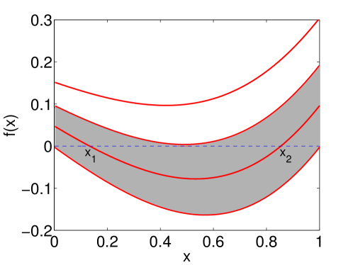
Figure 1: Annealed entropy density (leading order of logarithm of number of solution pairs $f(x)$ Eq. (5)), for $\alpha=0.8$, $p=0.4$, $k=2$. From top to bottom, $r$ values are $0.81r^{*}$, $0.8815r^{*}$, $0.94r^{*}$ and $r^{*}$ respectively. In the shaded regime $(0.8815r^{*},r^{*})$, $f(x)=0$ has two solutions, denoted by $x_{1}$ and $x_{2}$. One example of the two solutions are labeled in the figure for $r=0.94r^{*}$.

In Fig. 1 we plot $f(x)$ as a function of $x$ for $k=2$, $p=0.4$, $\alpha=0.8$ and several different $r$ values. The top line has a relatively small $r$, we can see that $f(x)$ is above $0$. It’s worth to mention this does not mean there are exponential number of solutions at distance $Nx$, because $f(x)$ is only a lower bound for $\ln(Z(x))/(N\ln N)$, indicated by Markov’s inequality

$$P(Z(x)\geq 0)\leq\mathbb{E}(Z(x)).$$

With $r$ increasing, this $f(x)$ curve becomes lower and lower. At a certain value $\hat{r}$, $=0.8815r^{*}$ in our example in Fig. 1, $f(x)$ curve reaches $0$. Beyond $\hat{r}$, $f(x)=0$ has $2$ solutions until $r$ reaches $r^{*}$. With $r>r^{*}$, it has been proved Xu, and Li that there is no solution in the system which is consistent with what the curve shows: the upper bound of $Z(x)$ becomes negative for any $x$ value.

We focus on the regime between $\hat{r}$ and $r^{*}$ (shaded regime in the figure) when $f(x)=0$ has two solutions, denoted by $x_{1}$ and $x_{2}$. Using definition of $f(x)$ in Eq. (5), we can compute number of solutions at Hamming distance between $x_{1}$ and $x_{2}$ with $N\to\infty$:

$$P\left(\sum_{xN=x_{1}N+1}^{x_{2}N-1}Z(x)\geq 0\right) \leq \mathbb{E}\left(\sum_{xN=x_{1}N+1}^{x_{2}N-1}{Z(x)}\right)$$ (6)

$$\leq (x_{2}-x_{1})N\cdot\max_{x\in(x_{1},x_{2})}{\mathbb{E}\left(Z(x)\right)}$$

$$\rightarrow (x_{2}-x_{1})N\cdot\max_{x\in(x_{1},x_{2})}{N^{f(x)N}}$$

$$\rightarrow 0.$$

Thus the last equation indicates that w.h.p. there is no solution pair at Hamming distance between $x_{1}$ and $x_{2}$.

On the other hand, with $N\to\infty$, using Paley-Zigmund inequality we have

$$P[X>\frac{1}{N}\mathbb{E}(X)] \geq \frac{\left(\mathbb{E}(X)-\frac{1}{N}\mathbb{E}(X)\right)^{2}}{\mathbb{E}(X^{2})}$$ (7)

$$\rightarrow (1-\frac{1}{N})^{2}\rightarrow 1,$$

where we have made use of Eq. (4) that $\lim_{N\to\infty}\frac{(\mathbb{E}(X))^{2}}{\mathbb{E}(X^{2})}=1$. The number of solutions $X$ is w.h.p. bigger than its mean divided by $N$.

It follows that w.h.p. in the regime where ($x_{1}$, $x_{2}$) pair exists (e.g. shaded regime in Fig. 1), system has exponentially number of solutions and their Hamming distance is discontinuously distributed. In other words, the solution space is clustered. Actually we can show that for all parameters of model RB, there always exists such clustered regime. A proof for the existence of $x_{1}$ and $x_{2}$ pair is given in Appendix A.

III.2 Organization of clusters

In this section we give a precise description on clustering of solutions, including bounds for diameter of clusters, distance between clusters, number of solutions in one cluster and number of clusters in the satisfiable phase. Given the result from last section, using method from Achlioptas and Ricci-Tersenghi (referring to section 3 of Achlioptas, and Ricci-Tersenghi , Achlioptas, coja-oghlan, and Tersenghi , section 3 of Achlioptas, and ), we actually have a concrete way to split the solution space and put solutions into different clusters: Assuming we know all the solutions, we can split the solution space by the cured surface $\{y|d(x,y)=x_{1}N\}$ for each solution, and obtain a set of regions $\mathbb{A}$. In more detail we can do it as follows:

1. Initialize $\mathbb{A}=\{\mathcal{S}\}$, with $\mathcal{S}$ denoting the set of all solutions.

2. For every solution $x\in\mathcal{S}$, repeat splitting step (step 3) around $x$.

3. Splitting step: denote the only region including $x$ in $\mathbb{A}$ by $A$. If there is $y\in A$ satisfied $d(x,y)>x_{1}N$, then let $B=\{y|y\in A,d(x,y)\leq x_{1}N\}$, $C=A\setminus B$, and let $\mathbb{A}=(\mathbb{A}\cup\{B\}\cup\{C\})\setminus\{A\}$.

The final $\mathbb{A}$ is the set of regions we want. We can show that $\mathbb{A}$ has following properties:

• The diameter of each region is at most $x_{1}N$. Because if there are two solutions at distance more than $x_{1}N$ in a region, splitting step will for sure split them into different regions.

• The distance between every pair of regions is at least $(x_{2}-x_{1})N$. To show this, assume there are three solutions $x$, $y$ and $z$, they are put into two clusters after the splitting step around $x$: $y$ is put to the same region with $x$, and $z$ is put to a different region. Then we have $d(x,y)\leq x_{1}N$, $d(x,z)\geq x_{2}N$, and the triangle rule implies that $d(y,z)\geq(x_{2}-x_{1})N$.

Another important property we are interested in is the number of solutions in clusters. Here for convenience we talk about typical instances of model RB, only to avoid repeatedly using of “w.h.p.”. From above analysis we know that the diameter of each region is at most $x_{1}N$, so number of solution pairs in one cluster is bounded above by number of solution pairs Hamming distance smaller than $x_{1}$. Letting

$$l=\max_{x\in[\frac{1}{N},x_{1}]}{\mathbb{E}(Z(x))}$$ (8)

and using Markov’s inequality we have

$$P\left(\sum_{xN=1}^{x_{1}N}{Z(x)}\geq N^{2}l\right)\leq\frac{\sum_{xN=1}^{x_{1}N}{\mathbb{E}(Z(x))}}{N^{2}l}\leq\frac{Nl}{N^{2}l}=\frac{1}{N}.$$ (9)

We can see that every region in $\mathbb{A}$ have at most $N^{2}l$ pairs of solutions, which implies that every region in $\mathbb{A}$ have at most $N\sqrt{l}$ solutions. We know that $f(x)$ is a concave function, and is monotonically decreasing with $x\in[0,x_{1}]$ (see Appendix A for a proof), so as $N$ is very large, number of solutions in one cluster is smaller than

$$N\sqrt{l}<N^{1/2[\alpha+r\ln(1-p)]N+1}.$$

Note that compared with the lower bound of total number of solutions $\frac{1}{N}\mathbb{E}(X)$ (Eq.(7)), number of solutions in one region is exponentially smaller. To make it more precise, if we define a complexity function $\Sigma$ representing leading order of logarithm of number of clusters divided by $N\log N$ (note that in our system, correct scaling for densities is $N\log N$), we have as $N$ is very large

$$\Sigma \geq \frac{1}{N\ln N}\ln\left(\frac{\frac{1}{N}\mathbb{E}(X)}{N\sqrt{l}}\right)$$ (10)

$$\geq \frac{1}{2}\left[\alpha+r\ln(1-p)\right]-\frac{2}{N}.$$

Last equation says that in the satisfiable phase, complexity is positive all the way down to the transition.

A direct implication from above results is that in whole parameter range, phase diagram of model RB does not contain condensed clustered phase, because there does not exist a set of finite number of clusters that contain almost all the solutions. In replica symmetry breaking theory, existence of clustering transition is indicated by $\hat{\Sigma}(m=1)>0$ and existence of condensation is indicated by $\hat{\Sigma}(m=1)<0$ where $\hat{\Sigma}$ denotes complexity which is leading order of logarithm of number of pure states as a function of Parisi parameter $m$ Krzakala et al. (2007). With Parisi parameter $m=1$, first step replica symmetry breaking solution actually gives equal weight to each pure state, thus the total free energy is identical to the replica symmetry free energy. We can see that our definition of complexity $\Sigma$ is very similar to $\hat{\Sigma}(m=1)$ because it gives equal weight to different clusters. Thus $\Sigma>0$ all the way down to the satisfiability transition is another way to show that there is no condensation transition in model RB. Note since our definition of clusters is different from pure state (as we do not refer to properties of Gibbs measure), our claim is not a proof.

IV conclusion and discussion

As a conclusion, in this paper we described in detail the solution space structure of model RB problem using rigorous methods. We show that close to the satisfiability transition, solutions clustered into exponential number of clusters, each of which contains sub-exponential number of solutions. And we showed that there is no condensation transition in model RB which testifies an statement of Zhao et al Zhao, Zhang, Zheng, and Xu using non-rigorous cavity methods from statistical physics.

The factor graph of model RB has a special feature that the link degree per variable is very large (growing with number of variables $N$), which is the same as model K-SAT with growing K Fri . We think this feature will affect phase transitions, and we will put more thoughts on that in future work.

We note that though we proved the clustering of solutions close to the satisfiability transition, we are still not sure where the clustered phase begins. Though lack of rigorous methods, heuristically the clustering transition can be estimated when one step replica symmetry breaking cavity method at Parisi parameter $m=1$ begins to have non-trivial solution. We will address this point in future work.

It has been shown that instead of clustering, freezing of clusters is the real reason for algorithmic hardness. Numerical experiments made in Zhao, Zhang, Zheng, and Xu and Zhao, Zhang, Zheng, and Xu showed that starting from $\hat{r}$ (where $f(x)=0$ has only one solution), the most efficient algorithms begin to fail in finding solutions, so it suggests that clusters become frozen immediately at $\hat{r}$. This would be interesting to study in detail.

V Acknowledgments

Pan Zhang wishes to thank Cristopher Moore for helpful conversations.

Appendix A Concavity of $f(x)$

The first and second derivatives of $f(x)$ with respect to $x$ read

$$\frac{\partial f}{\partial x} = \alpha-\frac{rpk(1-x)^{k-1}}{1-p+p(1-x)^{k}}$$

$$\frac{\partial^{2}f}{\partial x^{2}} = \frac{rpk}{\left[1-p+p(1-x)^{k}\right]^{2}}\left[(k-1)(1-p)(1-x)^{k-2}-p(1-x)^{2k-2}\right].$$

Then it is easy to check that $\frac{\partial^{2}f}{\partial x^{2}}$ is always positive for $x\in[0,1]$ with $k\geq 2$ and $p\leq 1-\frac{1}{k}$, which implies the concavity of $f(x)$.

Observe that both $f(0)$ and $f(1)$ are positive in the satisfiable phase, $f(0)=f(1)=0$ at the satisfiable-unsatisfiable transition, and $\left.\frac{\partial f(x)}{\partial x}\right|_{x=1}=\alpha>0.$ So using the concavity of $f(x)$, it is obvious that there must exist $r<r^{*}$, and pair $x_{1},x_{2}$ such that $f(x)<0$ with $x_{1}<x<x_{2}$. Moreover in the satisfiable phase, given $f(0)=\alpha+r\ln(1-p)>0$ and $x_{1}$ is the first point that $f(x)$ reaches $0$, we can conclude that $f(x)$ is a monotonically decreasing function with $x\in[0,x_{1}]$.

References

- (1) S. Kirkpatrick, and B. Selman, Science 264, 1297-1301 (1994).
- (2) R. Monasson, R. Zecchina, S. Kirkpatrick, B. Selman, and L. Troyansky, Nature 400, 133-137 (1999).
- (3) M. Mézard, G. Parisi, and R. Zecchina, Science 297, 812 (2002).
- Mézard and Zecchina (2002) M. Mézard and R. Zecchina, Phys. Rev. E 66, 056126 (2002).
- Mézard and Parisi (2002) M. Mézard and G. Parisi, Eur. Phys. J. B 20, 217 (2001).
- Krzakala et al. (2007) F. Krzakala, A. Montanari, F. Ricci-Tersenghi, G. Semerjian, and L. Zdeborova, in Proc. Natl. Acad. Sci. USA (2007), vol. 104 , pp. 10318.
- (7) A. Montanari, F. Ricci-Tersenghi, and G. Semerjian, J. Stat. Mech.: Theory Exp. (2008) P04004.
- (8) L. Zdeborova, and F. Krzakala, Phys. Rev. E (2007), vol. 76 , 031131.
- (9) M. Mézard, T. Mora, and R. Zecchina, Phys. Rev. Lett. 94, 197205 (2005).
- (10) D. Achlioptas, A. Coja-Oghlan, and F. Ricci-Tersenghi, Rand. Struct. Algorithms 38, 251 (2011).
- (11) D. Achlioptas, and A. Coja-Oghlan, in Proc. 49th FOCS (2008), pp. 793-802.
- (12) A. Coja-Oghlan, and L. Zdeborova, Proc. 23rd SODA (2011), pp. 241-250.
- (13) K. Xu and W. Li, J. Artif. Intell. Res. 12, 93 (2000).
- (14) B. Smith and M. Dyer, Artif. Intell. 81, 155 (1996).
- (15) K. Xu and W. Li, Theor. Comput. Sci. 355, 291 (2006).
- (16) K. Xu, F. Boussemart, F. Hemery, and C. Lecoutre, Artif. Intell. 171, 514 (2007).
- (17) T. Liu, X. Lin, and C. Wang, in IJCAI (2011), pp. 611-616.
- (18) C. Y. Zhao, H. J. Zhou, Z. M. Zheng, and K. Xu, J. Stat. Mech.: Theory Exp. (2011) P02019.
- (19) C. Y. Zhao, P. Zhang, Z. M. Zheng, and K. Xu, Phys. Rev. E 85, 016106 (2012).
- (20) D. Achlioptas, and C. Moore, SIAM J. Computing 36, 740-762 (2006).
- Lecoutre and (2009) C. Lecoutre Constraint Networks: Techniques and Algorithms (ISTE Ltd, London, 2009).
- (22) B. Smith, Theoretical Computer Science 265, 265-283 (2001).
- (23) A. Frieze, and M. Molloy, Proc. Random 03 (2003), pp. 275-289.
- (24) Y. Fan, and J. Shen, Artif Intell 175, 914-927 (2011).
- (25) Y. Fan, J. Shen, and K. Xu, Artif Intell 193, 1-17 (2012).
- (26) P. Zhang, Y. Zeng, and H. Zhou, Phys. Rev. E 80, 021122 (2009).
- (27) J. Barbier, F. Krzakala, L. Zdeborova, and P. Zhang, Journal of Physics: Conference Series 473, 012021 (2013).
- (28) D. Achlioptas, and F. Ricci-Tersenghi, Proc. STOC’06 (2006), pp. 130-139.
- (29) D. Achlioptas, Eur. Phys. J. B 64, 395 (2008).
- (30) A. M. Frieze, and N. C. Wormald, Combinatorica 25(3), 297-305 (2005).