Exploring dark matter microphysics with galaxy surveys
Abstract
We use present cosmological observations and forecasts of future experiments to illustrate the power of large-scale structure (LSS) surveys in probing dark matter (DM) microphysics and unveiling potential deviations from the standard CDM scenario. To quantify this statement, we focus on an extension of CDM with DM–neutrino scattering, which leaves a distinctive imprint on the angular and matter power spectra. After finding that future CMB experiments (such as COrE+) will not significantly improve the constraints set by the Planck satellite, we show that the next generation of galaxy clustering surveys (such as DESI) could play a leading role in constraining alternative cosmologies and even have the potential to make a discovery. Typically we find that DESI would be an order of magnitude more sensitive to DM interactions than Planck, thus probing effects that until now have only been accessible via -body simulations.
I Introduction
Dark matter (DM) is required to explain the galactic rotation curves, lensing and virial motions of galaxy clusters, observed matter power spectrum and cosmic microwave background (CMB) acoustic peaks. The current paradigm is that DM can be well-approximated by a collisionless fluid, consisting of weakly-interacting massive particles (WIMPs) and leading to a characteristic matter power spectrum (). However, direct evidence for WIMPs remains elusive and it is now legitimate to question the validity of the standard picture.
The CDM framework provides an excellent fit to the currently-available data Ade et al. (2014); Adam et al. (2015). Any future rejection or modification of this model must therefore come in the form of comparison with a (better) alternative hypothesis, or through the discovery of new data in direct conflict with CDM predictions. Possible modifications to the Standard Model either assume new relativistic species such as sterile neutrinos Dodelson and Widrow (1994); Lesgourgues and Pastor (2006), or different DM characteristics such as interactions with particles in the visible or dark sector. Either way, these “Beyond the Standard Model” scenarios predict a modification of the CDM matter power spectrum at small scales.
There is in fact a plethora of DM models in the literature that exhibit such deviations (e.g. Refs. Boehm et al. (2001, 2002); Boehm and Schaeffer (2005); Bertschinger (2006); Mangano et al. (2006); Serra et al. (2010); Wilkinson et al. (2014a); van den Aarssen et al. (2012); Farzan and Palomares-Ruiz (2014); Boehm et al. (2014); Cherry et al. (2014); Bertoni et al. (2015); Schewtschenko et al. (2015); Davis and Silk (2015); Sigurdson et al. (2004); Wilkinson et al. (2014b); Dolgov et al. (2013); Chen et al. (2002); Dvorkin et al. (2014); Park et al. (2012); Diamanti et al. (2013); Blennow et al. (2012); Cyr-Racine et al. (2014)), many of which predict additional damping and/or oscillations in the . While CMB experiments such as Planck allow one to constrain the cosmological parameters with unprecedented precision Ade et al. (2014); Adam et al. (2015), extracting the from Planck or the next-generation of CMB probes (such as COrE+ Bouchet et al. (2011) or PIXIE Kogut et al. (2011)) will be limited by the large uncertainties involved in foreground modelling, which hinder any angular power spectrum analysis at large 111An additional difficulty is that the are the result of the convolution of the with a window (Bessel) function that accounts for the angular scale, thus preventing one from detecting small features in the .. Therefore, to unravel the nature of DM, a direct probe of the is needed. Here we show that the next generation of large-scale structure (LSS) surveys could provide us with key information on the particle properties of DM, due to their extremely high precision.
Galaxy clustering surveys Anderson et al. (2014a, b); Beutler et al. (2011); Blake et al. (2011); Padmanabhan et al. (2012); Percival et al. (2010); Parkinson et al. (2012) have already observed the imprint of Baryon Acoustic Oscillations (BAOs), a standard ruler to measure the Hubble expansion rate, , and the angular diameter distance, . Recently, the Baryon Oscillation Spectroscopic Survey (BOSS) collaboration Dawson et al. (2013) reported a separate extraction of and to a precision of 1% Anderson et al. (2014a). Here we show that by exploiting all of the information contained in the shape of the full (rather than solely the BAO geometrical signature Hamann et al. (2010); Giusarma et al. (2013a, b)), one can test the validity of the CDM model at scales below a Mpc.
For concreteness, we focus on one specific scenario, in which DM scatters elastically with the active neutrinos (hereafter, CDM) Boehm et al. (2001, 2002); Boehm and Schaeffer (2005); Bertschinger (2006); Mangano et al. (2006); Serra et al. (2010); Wilkinson et al. (2014a); van den Aarssen et al. (2012); Farzan and Palomares-Ruiz (2014); Boehm et al. (2014); Cherry et al. (2014); Bertoni et al. (2015); Schewtschenko et al. (2015); Davis and Silk (2015). Such a DM candidate erases small-scale perturbations through collisional damping Boehm et al. (2001); Boehm and Schaeffer (2005) and suppresses neutrino free-streaming in the early universe. This leaves a unique signature in the angular and matter power spectra and provides us with a framework to quantify the potential of future LSS surveys to constrain DM microphysics. We exploit both the current publicly available galaxy power spectrum data (in particular, from the WiggleZ survey Parkinson et al. (2012)) and the expected full-shape power spectrum measurements from the forthcoming Dark Energy Spectroscopic Instrument (DESI) Levi et al. (2013).
The structure of the paper is as follows. In Sec. II, we describe the CDM scenario. In Sec. III, we compute up-to-date constraints using both CMB data from Planck and full-shape LSS data from the WiggleZ survey. In Sec. IV, we perform a forecast of the sensitivity of planned experiments such as COrE+ and DESI to the CDM framework (and any model that generates small deviations from CDM). Finally, we draw our main conclusions in Sec. V.
II Dark matter–neutrino interactions
In the CDM scenario, DM remains in kinetic contact with the neutrino sector long after the chemical freeze-out (see Refs. Boehm et al. (2001, 2002); Boehm and Schaeffer (2005); Bertschinger (2006); Mangano et al. (2006); Serra et al. (2010); Wilkinson et al. (2014a); van den Aarssen et al. (2012); Farzan and Palomares-Ruiz (2014); Boehm et al. (2014); Cherry et al. (2014); Bertoni et al. (2015); Schewtschenko et al. (2015); Davis and Silk (2015) for previous related work). Small-scale DM perturbations are then erased as a result of ongoing elastic scattering through “collisional damping” Boehm et al. (2001); Boehm and Schaeffer (2005), rather than slowly clustering under gravity. At the same time, neutrinos cannot free-stream as efficiently as in CDM and behave more like a relativistic perfect fluid. The main consequences are: (i) an enhancement of the CMB acoustic peaks and (ii) a reduction of small-scale power in the matter power spectrum Mangano et al. (2006); Serra et al. (2010); Wilkinson et al. (2014a).
DM–neutrino interactions do not affect the background equations but they do modify the evolution of the DM and neutrino fluctuations. They can be implemented by a modification of the Euler equations. In the conformal Newtonian gauge222In analogy to the perturbation equations governing baryon–photon interactions, see e.g. Ref. Ma and Bertschinger (1995).,
| (1) | |||||
where , and are the density, velocity and shear perturbations respectively, refer to higher () neutrino moments, is the gravitational potential, is the conformal Hubble parameter and .
The key quantity in Eq. (1) is , which can be written in terms of the dimensionless quantity defined as
| (2) |
This variable describes the ratio of the DM–neutrino elastic scattering cross section, , to the DM mass, , normalised to the Thomson cross section, (see Ref. Boehm et al. (2002)). In our analyses, we will consider both s-wave ( constant) and p-wave () cross sections. For p-wave cross sections, we can write , where is the present-day value and is the cosmological scale factor, normalised to unity today. The larger the value of , the greater the suppression in the linear matter power spectrum with respect to CDM, for a given wavenumber , as shown in Fig. 1 (and can also be seen in Refs. Mangano et al. (2006); Serra et al. (2010); Wilkinson et al. (2014a)).
DM interactions leave a further imprint in the galaxy power spectrum through damped acoustic oscillations, which, in general, show up at smaller scales than those illustrated in Fig. 1. They were first pointed out in the context of DM–photon interactions (in the weak-coupling regime) in Ref. Boehm et al. (2002) and were later observed in interactions with baryons Chen et al. (2002), neutrinos Mangano et al. (2006); Serra et al. (2010) and dark radiation Diamanti et al. (2013); Blennow et al. (2012). They arise because the DM fluid acquires a non-zero pressure as a result of interactions with the thermal bath and are therefore similar to the photon–baryon fluid before recombination. Although they cannot be observed using current data, they provide a characteristic signature for future experiments.
However, in addition to the models mentioned above, damped oscillations in the are also expected for certain types of self-interacting DM Atrio-Barandela and Davidson (1997), late-forming DM Das and Weiner (2011) and atomic DM Cyr-Racine and Sigurdson (2013). Taking all these possibilities into account, it would be difficult to determine the specific nature of the DM coupling from this feature alone. Furthermore, since the oscillations are not as prominent as in the case of DM–photon interactions Boehm et al. (2002) or atomic DM in the sDAO (strong dark acoustic oscillation) scenario Buckley et al. (2014), they may not be resolved. In this case, there could be a degeneracy with both warm DM Viel et al. (2005) and axion DM Hlozek et al. (2015) models, which predict a sharp cut-off in the matter power spectrum at small scales.
III Current constraints
To assess how powerful the constraints from future LSS surveys can be, we first derive the limits set by current CMB and galaxy clustering surveys. These will then serve as a benchmark for our forecasts in Sec. IV.
To perform this analysis, the modifications shown in Eq. (1) are implemented in the Boltzmann code class Lesgourgues (2011) (see also Ref. Wilkinson et al. (2014a)) and the posterior likelihoods are obtained using the Markov Chain Monte Carlo (MCMC) code Monte Python Audren et al. (2013). The prior ranges for these parameters are listed in Tab. 1. Since can vary by many orders of magnitude, we select a logarithmic prior distribution for this parameter, in contrast to the linear priors used in Refs. Mangano et al. (2006); Serra et al. (2010); Wilkinson et al. (2014a).
| Parameter | Prior |
|---|---|
| log (s-wave) | |
| log (p-wave) |
For simplicity, we assume massless neutrinos333This is in contrast to Planck, whose analysis assumes two massless and one massive neutrino with eV Ade et al. (2014). Such a small neutrino mass only affects the CMB through a slight shift in the angular diameter distance, which can be exactly compensated by a decrease in of Ade et al. (2014) . and fix the effective number of neutrino species, , to the standard value of 3.046 Mangano et al. (2005). We have verified that allowing to vary has an impact on the value of the Hubble parameter, , but does not change the sensitivity to the parameter.
The current CMB constraints (using Planck 2013 + WMAP polarisation data Ade et al. (2014)) are shown in Tab. 2. The corresponding upper limits on the DM–neutrino scattering cross section (at 95% CL) are
| (3) |
if s-wave and
| (4) |
if p-wave. These results are consistent with those quoted by the authors of Refs. Mangano et al. (2006); Serra et al. (2010), with the caveat that they did not perform a full MCMC analysis.
| s-wave () | p-wave () | ||||
|---|---|---|---|---|---|
| Parameter | Planck 2013 | COrE+ | Planck 2013 | COrE+ | |
| (95% CL) | (95% CL) | (95% CL) | (95% CL) | ||
We now repeat the previous analysis adding LSS data on the full shape of the matter power spectrum. Concretely, we use the galaxy clustering information from the WiggleZ Dark Energy Survey Parkinson et al. (2012). The WiggleZ sample consists of galaxies and covers a region of 1 in redshift space. Our calculations have shown that comparable results can be obtained from the BOSS DR11 measurements Anderson et al. (2014a). Following a similar analysis to Ref. Reid et al. (2010), we construct the likelihood function as follows:
| (5) |
where the covariance matrix reads
| (6) |
and
| (7) |
In Eq. (7), is the measured galaxy power spectrum and is the theoretical expectation for the set of model parameters , listed in Tab. 1. In turn, is a convolution of the computed galaxy power spectrum with the survey window functions, , and is given by
| (8) |
In this equation, represents the scaling, which takes into account that the observed galaxy redshift has to be translated into a distance using a fiducial model. In this case, we use the same values as in Ref. Riemer-Sorensen et al. (2012): , , , and . The scaling factor is given by Refs. Tegmark et al. (2006); Reid et al. (2010):
| (9) |
The theoretical galaxy power spectrum is related to the matter power spectrum through the relation
| (10) |
where is the bias, which is assumed to be constant. We analytically marginalise over as in Ref. Lewis and Bridle (2002):
| (11) |
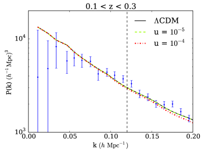
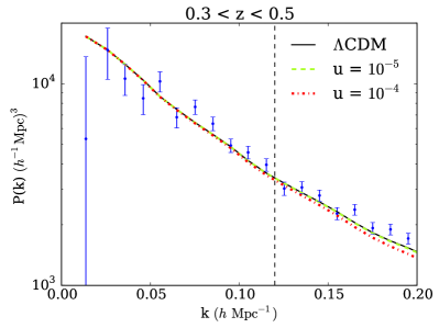
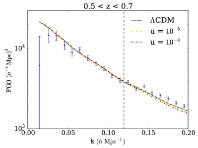
In Fig. 1, we show the measured galaxy power spectrum, , from WiggleZ in the four redshift bins (, , and ) exploited in our analyses Parkinson et al. (2012). We also depict the convolved power spectrum, , as defined in Eq. (8), for the CDM fiducial model of Ref. Riemer-Sorensen et al. (2012) and for two values of the parameter ( and , both in the s-wave scenario). The characteristic damping of the due to the interacting DM–neutrino fluid is clearly visible and allows us to tighten the constraints with respect to the previous CMB-only analysis.
| s-wave () | p-wave () | ||||
|---|---|---|---|---|---|
| Parameter | Mpc-1 | Mpc-1 | Mpc-1 | Mpc-1 | |
| (95% CL) | (95% CL) | (95% CL) | (95% CL) | ||
 |
 |
 |
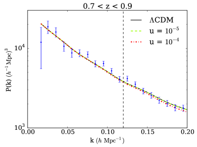 |
In Tab. 3, we present the posteriors obtained using the combination of WiggleZ and CMB data. We perform two separate analyses, including data for which: (i) Mpc-1 (purely linear regime) and (ii) Mpc-1 (weakly non-linear regime).
In terms of the DM–neutrino scattering cross section (at 95% CL) with Mpc-1 ( Mpc-1), we obtain
| (12) |
for the s-wave cross section. As we shall see in the next section, these bounds are competitive with those resulting from our forecasts for the future CMB mission COrE+.
Meanwhile, for the p-wave cross section, we obtain
| (13) |
Therefore, including data in the weakly non-linear regime ( Mpc-1) only strengthens the constraints by a factor of (s-wave) and (p-wave) with respect to those in the purely linear regime ( Mpc-1). We note that, in the s-wave scenario, the bounds are as much as times tighter than those using only CMB measurements, showing the benefits of utilising the full shape of the . The improvement is not as significant for the p-wave case because the suppression appears at larger scales (see e.g. Ref. Blennow et al. (2012)).
IV Forecasts for future experiments
The CMB and LSS analyses in Sec. III allowed us to obtain current constraints on the DM–neutrino elastic scattering cross section. We will now assess the power of future experiments in (i) constraining DM microphysics and (ii) detecting small deviations from the CDM matter power spectrum in the weakly non-linear regime. These two analyses require slightly different methodologies. In the first case, we construct a mock catalogue based on the CDM cosmology and compute the strongest possible upper limit on the parameter using the expected sensitivity of future experiments. In the second case, the mock data assumes small but non-negligible DM–neutrino interactions in order to assess our ability to detect them and more generally, reconstruct possible deviations from CDM. In both cases, we use projected sensitivities.
As in the previous section, we first consider CMB observables only and then include data from LSS surveys. We focus on two planned experiments: (i) COrE+ Bouchet et al. (2011), a CMB space mission currently proposed for the 2015-2025 ESA call, and (ii) DESI Levi et al. (2013), a multiplexed fibre-fed spectrograph to detect galaxies and quasars up to redshift , that is expected to run in the 2018-2022 timeframe.
IV.1 COrE+
We first produce full mock CMB data sets (temperature and -polarisation, plus lensing). We then compute the fiducial angular power spectra, , using the best-fit cosmology reported by the Planck 2015 final mission, including the TT, TE and EE spectra Adam et al. (2015). To these , we add a noise component consistent with each COrE+ channel specification and given by
| (14) |
where correspond to the temperature or polarisation errors (i.e. {T,E}). The expected temperature and polarisation sensitivities are given in Tab. 4.
Following Ref. Perotto et al. (2006), the effective is given by
| (15) |
where is a certain function of the noised power spectra (see Eq. (3.4) in Ref. Perotto et al. (2006)) and and represent the determinants of the theoretical and observed covariance matrices respectively. Finally, represents the observed fraction of the sky (in practice, it weights the correlations between multipoles when the map does not cover the full sky). For this analysis, we use Bouchet et al. (2011).
| Channel | T | P | |
|---|---|---|---|
| (GHz) | (arcmin) | (arcmin) | (arcmin) |
| 105 | 10.0 | 2.68 | 4.63 |
| 135 | 7.8 | 2.63 | 4.55 |
| 165 | 6.4 | 2.67 | 4.61 |
| 195 | 5.4 | 2.63 | 4.54 |
The third step in our analysis is to compute a Gaussian likelihood around our fiducial spectra, using class, tuned to obtain a 0.01% precision on the (as in Ref. Perotto et al. (2006), according to Eq. (15) and with a noise given by Eq. (14)). Then, assuming a 4-year sensitivity and using Monte Python to sample the parameter space with the priors given in Tab. 1, we can predict the sensitivity of COrE+ to the CDM parameters. Note that we only consider the TT, TE and EE observables. For simplicity, we neglect tensor modes (i.e. BT, BE and BB) as they have currently not been observed Ade et al. (2015a).
The results are presented in Tab. 2. We infer that the future sensitivity of COrE+ to a DM–neutrino coupling would be (at 95% CL)
| (16) |
if s-wave and
| (17) |
if p-wave.
While we find that the standard cosmological parameters will be measured to much higher precision than with Planck, there is only a modest gain in sensitivity to the DM–neutrino cross section. Furthermore, these limits are slightly worse than those obtained after combining Planck with current LSS data in the weakly non-linear regime. From these results, we expect detection with COrE+ to be possible for .
To assess the power of COrE+ to detect and reconstruct the CDM cosmology or similar deviations to CDM, we also produce mock data sets with and as fiducial models (for s-wave interactions). We then attempt to reconstruct these models by means of the usual MCMC method. The case is presented in Fig. 2 (and similarly for p-wave with ). With COrE+–like CMB data, one may reconstruct a universe with with a error. However, the case would provide us with CMB information entirely consistent with , in agreement with Eq. (16). Therefore, is the best sensitivity that one could achieve with CMB experiments in the near future.
IV.2 DESI
The DESI survey Levi et al. (2013) is expected to provide a wealth of information on the matter distribution (i.e. the P) in the Universe at relatively small scales and up to redshift . To forecast the ability of DESI to discover new physics, we first compute the expected errors from the DESI instrument, following a Fisher matrix approach, which is the usual method used to forecast galaxy survey experiments444http://desi.lbl.gov/,555http://sci.esa.int/euclid/.
The Fisher matrix is defined as the expectation value of the second derivative of the likelihood surface around its maximum. As long as the posterior distribution for the parameters is well approximated by a multivariate Gaussian function, its elements are given by Tegmark et al. (1997); Jungman et al. (1996); Fisher (1935)
| (18) |
where is the total covariance, which consists of signal and noise terms. Once more, we take a fiducial cosmology defined by the parameters that best fit the Planck 2015 TT, TE, EE lowP data Ade et al. (2015b) in the presence of DM–neutrino interactions with in the s-wave scenario and in the p-wave scenario666See Ref. Seo and Eisenstein (2003) for more details on the Fisher matrix formalism for galaxy redshift surveys such as DESI..
Assuming a Gaussian likelihood for the DESI band powers, the Fisher matrix can be written as:
where is the effective volume of the survey and given by
| (20) |
where is the cosine of the angle between the vector mode () and the vector along the line of sight, and is the galaxy number density (which is assumed to be constant throughout each of the redshift bins).
To perform the analysis, we divide the data in redshift bins of width and cut the small-scale data at Mpc-1 to avoid the highly non-linear regime. The lowest wavenumber (i.e. the largest scale), , is chosen to be greater than , where represents the volume of the redshift shell. We note that using data in the non-linear regime would require numerical simulations of this model. This has been performed for specific cases in Refs. Boehm et al. (2014); Schewtschenko et al. (2015). As we will discuss later, constraints using this method are competitive with our DESI forecast.
The real-space linear DM power spectrum, , is related to the linear redshift-space galaxy power spectrum, , by
| (21) |
where is the bias relating galaxy to DM overdensities in real space (as in Eq. (10)) and is the linear growth factor.
DESI is expected to cover 14,000 deg2 of the sky in the redshift range . We use the values of the bias given in Ref. Font-Ribera et al. (2014) for the three types of DESI tracers, namely for the Emission Line Galaxies (ELGs), for the Luminous Red Galaxies (LRGs) and for the high redshift quasars (QSOs). Here, is the normalised growth factor and both the bias and the growth factor are assumed to vary in each redshift bin accordingly to these expressions. To combine the Fisher matrices from the three DESI tracers, we use the multi-tracer technique of Ref. Abramo and Leonard (2013).
For the s-wave scenario, we obtain a error on the parameter of
| (22) |
for the fiducial value of . For p-wave, we obtain:
| (23) |
for the fiducial value of . Crucially, DESI will ensure a detection of DM–neutrino interactions if the strength of such a coupling is (or a detection for if p-wave).
Our results are summarised in Fig. 2, where the DESI and CL allowed regions in the (,) plane are shown (assuming the Planck 2015 fiducial cosmology plus an interaction strength of if s-wave and if p-wave), along with the current constraints and the COrE+ reconstruction. One can clearly see the improvement in the extraction of a DM–neutrino coupling that will be provided by the next-generation LSS surveys. This analysis indicates that planned galaxy clustering surveys will provide an extremely powerful tool (competitive or even better than future CMB experiments) to test the fundamental properties of DM.
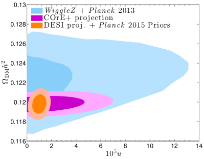
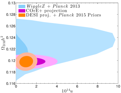
Since the main impact of CDM is the damping of structure on small scales, one of the largest effects will be a reduction in the number of satellites around galaxies such as the Milky Way. Until now, the only way to study interactions at these scales has been via -body simulations, which show that for DM–radiation couplings greater than , the number of satellites in the Milky Way would be much smaller than observed Boehm et al. (2014); Schewtschenko et al. (2015). Therefore, with the sensitivity of expected from DESI, we would have a handle on alternative scenarios to CDM that modify our cosmic neighbourhood, independently of the assumptions that go into -body simulations777With improvements in numerical algorithms and computing power, -body simulations are becoming increasingly more affordable and will continue to provide a complementary method to test structure formation in models beyond CDM. However, they will remain computationally expensive, especially if one wishes to simulate structures on both large and small scales or test a wide range of modifications to the P..
V Conclusion
Cosmology provides a promising tool to measure the particle properties of dark matter (DM). A DM coupling to visible or dark radiation (including neutrinos, axions, dark photons or any other light uncharged particle) can lead to strong departures from the standard CDM cosmology and produce visible signatures for CMB experiments and LSS surveys. In the specific case of DM–neutrino scattering, one expects an enhancement of the CMB acoustic peaks due to the fact that DM is strongly coupled to neutrinos and vice versa, which delays the neutrino free-streaming epoch and alters DM clustering with respect to the standard CDM picture. However, the largest impact is imprinted as a damping in the matter power spectrum, surveyed by large-scale structure (LSS) galaxy surveys.
In this study, we have looked for the optimal method to measure such small departures from the CDM scenario. As cosmological measurements may constitute the only tool available to detect such effects, it is crucial to study the potential sensitivity of future experiments. We have shown that i) with current CMB measurements, one can probe s-wave and p-wave DM–neutrino cross sections of and , respectively (at CL) and ii) by simulating a next-generation CMB experiment (i.e. a COrE+-like mission) by means of a Markov Chain Monte Carlo analysis, one can only weakly improve on the current sensitivity.
The prospects for both constraints and detection are far better for future galaxy surveys, such as the DESI or Euclid experiments. Already, current LSS data, combined with Planck CMB measurements, provide competitive constraints to those forecasted for a future CMB experiment such as COrE+. Future data from the DESI experiment alone could improve the current sensitivity limit by an order of magnitude, and provide an accurate (percent-level) measurement of the scattering cross section for values above that limit. Therefore, we have shown that galaxy clustering surveys are an excellent probe to detect new physics beyond CDM. Remarkably, future LSS experiments will be sensitive to effects that until now have only been accessible via -body simulations.
VI Acknowledgements
The authors would like to thank Andreu Ariño for useful discussions and Will Percival for precious BOSS DR11 measurements. The authors acknowledge the use of the publicly available numerical codes class and Monte Python, and the data from the Planck Legacy Archive and WiggleZ survey. ME is supported by Spanish grant FPU13/03111 of the MECD. RJW is supported by the STFC grant ST/K501979/1. This work was supported by the European Union FP7 ITN INVISIBLES (Marie Curie Actions, PITN-GA-2011-289442). We would like to thank the Universitad Autónoma de Madrid and IFT for hospitality while this work was completed.
References
- Ade et al. (2014) P. Ade et al. (Planck Collaboration), Astron.Astrophys. 571, A16 (2014), arXiv:1303.5076 [astro-ph.CO] .
- Adam et al. (2015) R. Adam et al. (Planck Collaboration), (2015), arXiv:1502.01582 [astro-ph.CO] .
- Dodelson and Widrow (1994) S. Dodelson and L. M. Widrow, Phys. Rev. Lett. 72, 17 (1994), arXiv:hep-ph/9303287 [hep-ph] .
- Lesgourgues and Pastor (2006) J. Lesgourgues and S. Pastor, Phys.Rept. 429, 307 (2006), arXiv:astro-ph/0603494 [astro-ph] .
- Boehm et al. (2001) C. Boehm, P. Fayet, and R. Schaeffer, Phys.Lett. B518, 8 (2001), arXiv:astro-ph/0012504 [astro-ph] .
- Boehm et al. (2002) C. Boehm, A. Riazuelo, S. H. Hansen, and R. Schaeffer, Phys.Rev. D66, 083505 (2002), arXiv:astro-ph/0112522 [astro-ph] .
- Boehm and Schaeffer (2005) C. Boehm and R. Schaeffer, Astron.Astrophys. 438, 419 (2005), arXiv:astro-ph/0410591 [astro-ph] .
- Bertschinger (2006) E. Bertschinger, Phys.Rev. D74, 063509 (2006), arXiv:astro-ph/0607319 [astro-ph] .
- Mangano et al. (2006) G. Mangano, A. Melchiorri, P. Serra, A. Cooray, and M. Kamionkowski, Phys.Rev. D74, 043517 (2006), arXiv:astro-ph/0606190 [astro-ph] .
- Serra et al. (2010) P. Serra, F. Zalamea, A. Cooray, G. Mangano, and A. Melchiorri, Phys.Rev. D81, 043507 (2010), arXiv:0911.4411 [astro-ph.CO] .
- Wilkinson et al. (2014a) R. J. Wilkinson, C. Boehm, and J. Lesgourgues, JCAP 1405, 011 (2014a), arXiv:1401.7597 [astro-ph.CO] .
- van den Aarssen et al. (2012) L. G. van den Aarssen, T. Bringmann, and C. Pfrommer, Phys.Rev.Lett. 109, 231301 (2012), arXiv:1205.5809 [astro-ph.CO] .
- Farzan and Palomares-Ruiz (2014) Y. Farzan and S. Palomares-Ruiz, JCAP 1406, 014 (2014), arXiv:1401.7019 [hep-ph] .
- Boehm et al. (2014) C. Boehm, J. Schewtschenko, R. Wilkinson, C. Baugh, and S. Pascoli, Mon.Not.Roy.Astron.Soc. 445, L31 (2014), arXiv:1404.7012 [astro-ph.CO] .
- Cherry et al. (2014) J. F. Cherry, A. Friedland, and I. M. Shoemaker, (2014), arXiv:1411.1071 [hep-ph] .
- Bertoni et al. (2015) B. Bertoni, S. Ipek, D. McKeen, and A. E. Nelson, JHEP 1504, 170 (2015), arXiv:1412.3113 [hep-ph] .
- Schewtschenko et al. (2015) J. Schewtschenko, R. Wilkinson, C. Baugh, C. Boehm, and S. Pascoli, Mon.Not.Roy.Astron.Soc. 449, 3587 (2015), arXiv:1412.4905 [astro-ph.CO] .
- Davis and Silk (2015) J. H. Davis and J. Silk, (2015), arXiv:1505.01843 [hep-ph] .
- Sigurdson et al. (2004) K. Sigurdson, M. Doran, A. Kurylov, R. R. Caldwell, and M. Kamionkowski, Phys.Rev. D70, 083501 (2004), arXiv:astro-ph/0406355 [astro-ph] .
- Wilkinson et al. (2014b) R. J. Wilkinson, J. Lesgourgues, and C. Boehm, JCAP 1404, 026 (2014b), arXiv:1309.7588 [astro-ph.CO] .
- Dolgov et al. (2013) A. Dolgov, S. Dubovsky, G. Rubtsov, and I. Tkachev, Phys.Rev. D88, 117701 (2013), arXiv:1310.2376 [hep-ph] .
- Chen et al. (2002) X.-l. Chen, S. Hannestad, and R. J. Scherrer, Phys.Rev. D65, 123515 (2002), arXiv:astro-ph/0202496 [astro-ph] .
- Dvorkin et al. (2014) C. Dvorkin, K. Blum, and M. Kamionkowski, Phys.Rev. D89, 023519 (2014), arXiv:1311.2937 [astro-ph.CO] .
- Park et al. (2012) C.-G. Park, J.-c. Hwang, and H. Noh, Phys.Rev. D86, 083535 (2012), arXiv:1207.3124 [astro-ph.CO] .
- Diamanti et al. (2013) R. Diamanti, E. Giusarma, O. Mena, M. Archidiacono, and A. Melchiorri, Phys.Rev. D87, 063509 (2013), arXiv:1212.6007 [astro-ph.CO] .
- Blennow et al. (2012) M. Blennow, E. Fernandez-Martinez, O. Mena, J. Redondo, and P. Serra, JCAP 1207, 022 (2012), arXiv:1203.5803 [hep-ph] .
- Cyr-Racine et al. (2014) F.-Y. Cyr-Racine, R. de Putter, A. Raccanelli, and K. Sigurdson, Phys.Rev. D89, 063517 (2014), arXiv:1310.3278 [astro-ph.CO] .
- Bouchet et al. (2011) F. Bouchet et al. (COrE Collaboration), (2011), arXiv:1102.2181 [astro-ph.CO] .
- Kogut et al. (2011) A. Kogut, D. Fixsen, D. Chuss, J. Dotson, E. Dwek, et al., JCAP 1107, 025 (2011), arXiv:1105.2044 [astro-ph.CO] .
- Anderson et al. (2014a) L. Anderson et al. (BOSS), Mon.Not.Roy.Astron.Soc. 441, 24 (2014a), arXiv:1312.4877 [astro-ph.CO] .
- Anderson et al. (2014b) L. Anderson, E. Aubourg, S. Bailey, F. Beutler, A. S. Bolton, et al., Mon.Not.Roy.Astron.Soc. 439, 83 (2014b), arXiv:1303.4666 [astro-ph.CO] .
- Beutler et al. (2011) F. Beutler, C. Blake, M. Colless, D. H. Jones, L. Staveley-Smith, et al., Mon.Not.Roy.Astron.Soc. 416, 3017 (2011), arXiv:1106.3366 [astro-ph.CO] .
- Blake et al. (2011) C. Blake, E. Kazin, F. Beutler, T. Davis, D. Parkinson, et al., Mon.Not.Roy.Astron.Soc. 418, 1707 (2011), arXiv:1108.2635 [astro-ph.CO] .
- Padmanabhan et al. (2012) N. Padmanabhan, X. Xu, D. J. Eisenstein, R. Scalzo, A. J. Cuesta, et al., Mon.Not.Roy.Astron.Soc. 427, 2132 (2012), arXiv:1202.0090 [astro-ph.CO] .
- Percival et al. (2010) W. J. Percival et al. (SDSS), Mon.Not.Roy.Astron.Soc. 401, 2148 (2010), arXiv:0907.1660 [astro-ph.CO] .
- Parkinson et al. (2012) D. Parkinson, S. Riemer-Sorensen, C. Blake, G. B. Poole, T. M. Davis, et al., Phys.Rev. D86, 103518 (2012), arXiv:1210.2130 [astro-ph.CO] .
- Dawson et al. (2013) K. S. Dawson et al. (BOSS), Astron.J. 145, 10 (2013), arXiv:1208.0022 [astro-ph.CO] .
- Hamann et al. (2010) J. Hamann, S. Hannestad, J. Lesgourgues, C. Rampf, and Y. Y. Wong, JCAP 1007, 022 (2010), arXiv:1003.3999 [astro-ph.CO] .
- Giusarma et al. (2013a) E. Giusarma, R. De Putter, and O. Mena, Phys.Rev. D87, 043515 (2013a), arXiv:1211.2154 [astro-ph.CO] .
- Giusarma et al. (2013b) E. Giusarma, R. de Putter, S. Ho, and O. Mena, Phys.Rev. D88, 063515 (2013b), arXiv:1306.5544 [astro-ph.CO] .
- Levi et al. (2013) M. Levi et al. (DESI), (2013), arXiv:1308.0847 [astro-ph.CO] .
- Ma and Bertschinger (1995) C.-P. Ma and E. Bertschinger, Astrophys.J. 455, 7 (1995), arXiv:astro-ph/9506072 [astro-ph] .
- Atrio-Barandela and Davidson (1997) F. Atrio-Barandela and S. Davidson, Phys. Rev. D55, 5886 (1997), arXiv:astro-ph/9702236 [astro-ph] .
- Das and Weiner (2011) S. Das and N. Weiner, Phys. Rev. D84, 123511 (2011), arXiv:astro-ph/0611353 [astro-ph] .
- Cyr-Racine and Sigurdson (2013) F.-Y. Cyr-Racine and K. Sigurdson, Phys.Rev. D87, 103515 (2013), arXiv:1209.5752 [astro-ph.CO] .
- Buckley et al. (2014) M. R. Buckley, J. Zavala, F.-Y. Cyr-Racine, K. Sigurdson, and M. Vogelsberger, Phys. Rev. D90, 043524 (2014), arXiv:1405.2075 [astro-ph.CO] .
- Viel et al. (2005) M. Viel, J. Lesgourgues, M. G. Haehnelt, S. Matarrese, and A. Riotto, Phys. Rev. D71, 063534 (2005), arXiv:astro-ph/0501562 [astro-ph] .
- Hlozek et al. (2015) R. Hlozek, D. Grin, D. J. Marsh, and P. G. Ferreira, Phys. Rev. D91, 103512 (2015), arXiv:1410.2896 [astro-ph.CO] .
- Lesgourgues (2011) J. Lesgourgues, (2011), arXiv:1104.2932 [astro-ph.IM] .
- Audren et al. (2013) B. Audren, J. Lesgourgues, K. Benabed, and S. Prunet, JCAP 1302, 001 (2013), arXiv:1210.7183 [astro-ph.CO] .
- Mangano et al. (2005) G. Mangano, G. Miele, S. Pastor, T. Pinto, O. Pisanti, et al., Nucl.Phys. B729, 221 (2005), arXiv:hep-ph/0506164 [hep-ph] .
- Reid et al. (2010) B. A. Reid, W. J. Percival, D. J. Eisenstein, L. Verde, D. N. Spergel, et al., Mon.Not.Roy.Astron.Soc. 404, 60 (2010), arXiv:0907.1659 [astro-ph.CO] .
- Riemer-Sorensen et al. (2012) S. Riemer-Sorensen, C. Blake, D. Parkinson, T. M. Davis, S. Brough, et al., Phys.Rev. D85, 081101 (2012), arXiv:1112.4940 [astro-ph.CO] .
- Tegmark et al. (2006) M. Tegmark et al. (SDSS), Phys.Rev. D74, 123507 (2006), arXiv:astro-ph/0608632 [astro-ph] .
- Lewis and Bridle (2002) A. Lewis and S. Bridle, Phys.Rev. D66, 103511 (2002), arXiv:astro-ph/0205436 [astro-ph] .
- Perotto et al. (2006) L. Perotto, J. Lesgourgues, S. Hannestad, H. Tu, and Y. Y. Wong, JCAP 0610, 013 (2006), arXiv:astro-ph/0606227 [astro-ph] .
- Ade et al. (2015a) P. Ade et al. (Planck), (2015a), arXiv:1502.02114 [astro-ph.CO] .
- Tegmark et al. (1997) M. Tegmark, A. Taylor, and A. Heavens, Astrophys.J. 480, 22 (1997), arXiv:astro-ph/9603021 [astro-ph] .
- Jungman et al. (1996) G. Jungman, M. Kamionkowski, A. Kosowsky, and D. N. Spergel, Phys.Rev. D54, 1332 (1996), arXiv:astro-ph/9512139 [astro-ph] .
- Fisher (1935) R. A. Fisher, Journal of the Royal Statistical Society 98, pp. 39 (1935).
- Ade et al. (2015b) P. Ade et al. (Planck Collaboration), (2015b), arXiv:1502.01589 [astro-ph.CO] .
- Seo and Eisenstein (2003) H.-J. Seo and D. J. Eisenstein, Astrophys.J. 598, 720 (2003), arXiv:astro-ph/0307460 [astro-ph] .
- Font-Ribera et al. (2014) A. Font-Ribera, P. McDonald, N. Mostek, B. A. Reid, H.-J. Seo, et al., JCAP 1405, 023 (2014), arXiv:1308.4164 [astro-ph.CO] .
- Abramo and Leonard (2013) L. R. Abramo and K. E. Leonard, Mon.Not.Roy.Astron.Soc. 432, 318 (2013), arXiv:1302.5444 [astro-ph.CO] .