Seasonal Floquet states in a game-driven evolutionary dynamics

Abstract

Mating preferences of many biological species are not constant but season-dependent. Within the framework of evolutionary game theory this can be modeled with two finite opposite-sex populations playing against each other following the rules that are periodically changing. By combining Floquet theory and the concept of quasi-stationary distributions, we reveal existence of metastable time-periodic states in the evolution of finite game-driven populations. The evolutionary Floquet states correspond to time-periodic probability flows in the strategy space which cannot be resolved within the mean-field framework. The lifetime of metastable Floquet states increases with the size $N$ of populations so that they become attractors in the limit $N\rightarrow\infty$.

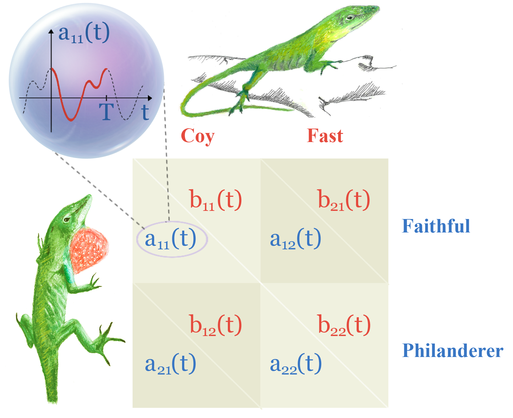
Introduction. The evolutionary dynamics of an animal group is tied to the reproductive activity of its members, a complex process which involves courtship rituals and sharing of parental care sexual . Within the game theory framework, the sex conflict over parental investment was formalized by Dawkins in his famous “Battle of Sexes” (BoS) dawkins , illustrated in Fig. 1. In this game two opposite-sex members of the group play against each other. Each player can use two behavioral strategies. Entries in the payoff matrix, $b_{ss^{\prime}}$, quantify the reward received by a female which used a strategy $s\in\{1,2\}$ after she has played against a male which used a strategy $s^{\prime}\in\{1,2\}$. Entries $a_{s^{\prime}s}$ define the reward of the male.

Figure 1: (color online) “Battle of Sexes” with seasonal variations. A female of Carolina anole lizards can be either coy and prefer an arduous courtship, to be sure that a mate is ready to contribute to a parental care, or fast, and thus not being much concerned about parental care of offspring. A male can be either faithful and ready to assure the female partner, by performing a long courtship, that he is a faithful potential husband, or philanderer and prefer to shorten the courtship stage. Depending on the strategies, $s$ ($s^{\prime}$), played by the female (male), the female (male) gets payoff $b_{ss^{\prime}}$ ($a_{s^{\prime}s}$). Both females and males are season-constrained in their strategies and preferences, which is modeled via time-periodic modulations of the payoffs.

A number of observations have shown that mating strategies and preferences of many species are not constant in time but season-dependent generic . For example, courtship srituals of the males of Carolina anole lizards (Anolis carolinensis), as well as mate selection criteria of the females of the species, are periodically changing during the year lizard1 . Even the amount of different types of muscle fibers that control the vibrations of a red throat fan (dewlap) - which males employ during the courtship - is a season dependent characteristic lizard2 . Currently, there is no agreement between the ecologists on the role this seasonal plasticity plays in determining the evolution direction of the species srev .

We address this problem within the BoS framework by allowing the payoffs to periodically vary in time, see Fig. 1. Our goal is to investigate how these modulations influence the game-driven evolutionary dynamics. Here, we first apply the concept of quasi-stationary distributions in absorbing Markov chains darroch to a stochastic evolutionary dynamics of finite populations and define the notion of evolutionary metastable states. Then, by employing the Floquet theory floquet ; floquetH , we generalize the notion of metastable states meta1 ; meta2 ; assaf to periodically modulated game-driven evolutionary dynamics. We show that in big but finite populations, the metastable Floquet states survive over extremely long (as compared to the period of modulations) timescales. We argue that, in the limit of infinitely big populations, these states become attractors while still evading the mean-field description.

Model. Finite size of animal populations favors a stochastic approach to evolutionary dynamics. Although the convergence to the deterministic mean-field dynamics is typically guaranteed in the limit $N\rightarrow\infty$ hof2 ; schlag , the stochastic dynamics of large but finite populations can still be very different from the mean-field picture traulsen1 ; traulsen2 ; traulsen3 ; frey . Here we adapt the game-oriented version of the Moran process moran , introduced in Ref. moranNature and generalized to two-player games in Ref. traulsen1 .

Players $A$ (males) and $B$ (females) form two populations, each one of a fixed size $N$ and with two available strategies, $s=\{1,2\}$, see Fig. 1. Game payoffs are time-periodic functions, $c_{ss^{\prime}}(t)=c_{ss^{\prime}}(t+T)$, $c=\{a,b\}$, and can be represented as sums of stationary and zero-mean time-periodic components, $c_{ss^{\prime}}(t)=\bar{c}_{ss^{\prime}}+\tilde{c}_{ss^{\prime}}(t)$, $\langle\tilde{c}_{ss^{\prime}}(t)\rangle_{T}=0$. The time starting from $t=0$ is incremented by $\triangle t=T/M$ after each round. After $M$ rounds the payoffs return to their initial values. The state of the populations after the $m$-th round is fully specified by the number of players playing the first strategy, $i$ (males) and $j$ (females), $0\leq i,j\leq N$. A detailed description of the corresponding stochastic process is given in Supplemental Material. It can also be shown that, in the limit $N\rightarrow\infty$ traulsen1 , the dynamics of the variables $x=i/N$ and $y=j/N$ is defined by the adjusted replicator equations generic ; see Refs. smith ; hof2 .

For a finite $N$, the state of the system can be expressed as a $N\times N$ matrix $\mathbf{p}$ with elements $p(i,j)$, which are the probabilities to find two populations in the states $i$ and $j$, respectively. Round-to-round dynamics can be evaluated by multiplying the state $\mathbf{p}$ with the transition fourth-order tensor $\mathbf{S}$, with elements $S(i,j,i^{\prime},j^{\prime})$ generic . By using the bijection $k=(N-1)j+i$, we can unfold the probability matrix $p(i,j)$ into the vector $\tilde{p}(k)$, $k=0,...,N^{2}$, and the tensor $S(i,j,i^{\prime},j^{\prime})$ into the matrix $\tilde{S}(k,l)$. This reduces the problem to a Markov chain gant , $\tilde{\textbf{p}}^{m+1}=\tilde{\textbf{S}}^{m}\tilde{\textbf{p}}^{m}$, where $m$ is the number of the round to be played. The four states $(i=\{0,N\},j=\{0,N\})$ are absorbing states because the transition rates leading out of them equal zero generic . The absorbing states are attractors of the dynamics for any finite $N$, and the finite-size fluctuations will eventually drive a population to one of them dykman ; frey . This would imply a fixation, so that only one strategy survived in each of now monomorphic populations traulsen1 ; frey .

Figure 2: (color online) Metastable states of the stationary BoS game. In the mean-filed limit $N=\infty$, a trajectory spirals towards a fixed point $\left(\frac{1}{2},\frac{1}{2}\right)$, the Nash equilibrium of the game. For the finite $N$, metastable states are specified by their quasi-stationary probability density functions (pdf’s) (3d plots). For $N=200$ the pdf combines the results of the direct diagonalization of the $39~{}601\times 39~{}601$ matrix $\tilde{\mathbf{Q}}$ (left half of the pdf, this procedure was also used to obtain the function for $N=100$) and of the preconditioned stochastic sampling (right part of the pdf, this procedure was also used to obtain the function for $N=400$) generic . The baseline fitness $w=0.3$ (other parameters are given in the text).

We are interested in the dynamics before the fixation, so we merge the four states into a single absorbing state by summing the corresponding incoming rates. The boundary states, $(i=\{0,N\},j\in\{1,\cdots,N-1\})$ and $(i\in\{1,\cdots,N-1\},j=\{0,N\})$, can also be merged into this absorbing super-state: Once the population gets to the boundary, it will only move towards one of the two nearest absorbing states. By labeling the absorbing super-state with index $k=0$, we end up with a $(L+1)\times(L+1)$ matrix

$$\tilde{\mathbf{S}}^{m}=\begin{bmatrix}1&\bm{\varrho_{0}}^{m}\\ \mathbf{0}&\tilde{\mathbf{Q}}^{m},\end{bmatrix}$$ (1)

where $L=(N-1)^{2}$, $\bm{\varrho}_{0}^{m}$ is a vector of the incoming transition probabilities of the absorbing super-state, $\mathbf{0}$ is a $L\times 1$ zero vector, and $\tilde{\mathbf{Q}}^{m}$ is a $L\times L$ reduced transition matrix.

With Eq. (1), we arrive at the setup used by Darroch and Seneta to formulate the concept of quasi-stationary distributions darroch . There is the normalized right eigenvector of the reduced transition matrix $\tilde{\mathbf{Q}}^{m}$ with the maximum eigenvalue $\lambda$ FPT . By using the inverse bijection, we can transform this vector into a two-dimensional probability density function (pdf), i.e., a state, $\mathbf{d}$, with maximal mean absorption time. This state is the most resistant to the wash-out by the finite-size fluctuations and it remains near invariant, up to a uniform rescaling, under the action of the tensor ${\mathbf{S}}$. This is the metastable state of the evolutionary process.

Stationary case. As an example, we consider a game with payoffs $a_{11}$, $a_{22}$, $b_{12}$ and $b_{21}$ equal $1$, and payoffs $-1$ for the rest of strategies neumann . Figure 2 presents the numerically obtained metastable states of the game. We use two methods, the direct diagonalization of the reduced transition matrix, which is stationary in this case, $\tilde{\mathbf{Q}}^{m}\equiv\tilde{\mathbf{Q}}$, and preconditioned stochastic sampling generic . For $N=200$ we find an agreement between the results of the two methods. The means of the metastable state,

$$\bar{x}=\sum_{i,j=1}^{N-1}\frac{i}{N}\cdot d(i,j);~{}\bar{y}=\sum_{i,j=1}^{N-1}\frac{j}{N}\cdot d(i,j),$$ (2)

coincide with the Nash equilibrium nash for any $N$. However, the actual dynamics is determined by the metastable limit cycle encircling the equilibrium (this could be seen by performing short-run stochastic simulations); see Fig. 2. Within the Langevin-oriented approach to the dynamics of finite populations traulsen1 ; traulsen4 , the appearance of the metastable limit cycle can be interpreted as a stochastic Hopf bifurcation arnold (see also Ref. lindner for another interpretation). In the limit $N\rightarrow\infty$ the cycle collapses to the Nash equilibrium. Note, however, that the convergence to this limit is slow, as indicated by the width of the pdf for $N=400$.

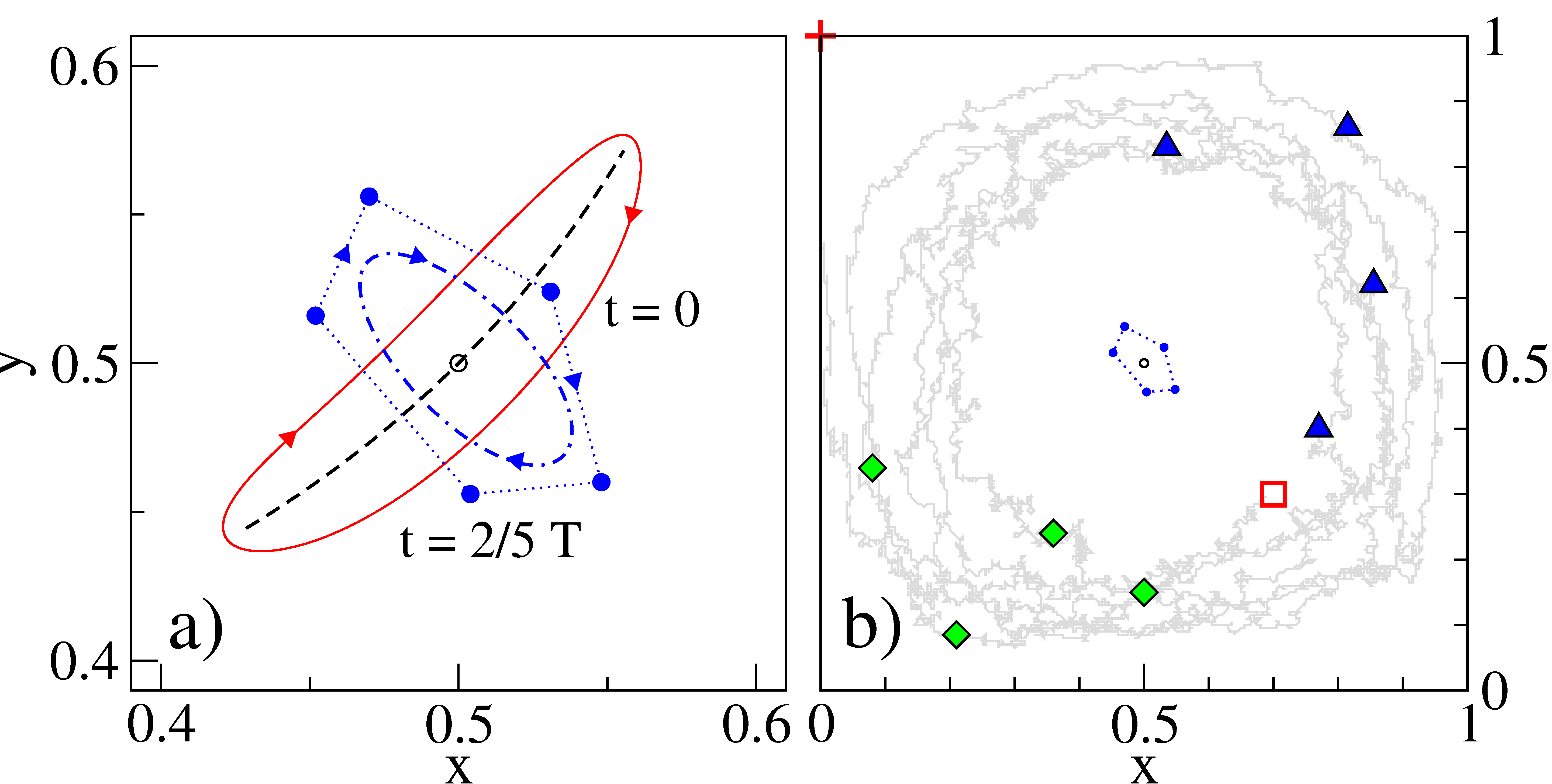
Case of modulated payoffs. By adding time-modulations to the model, we find that the mean-field dynamics does not exhibit substantial changes. For the choice $\epsilon(t)=\tilde{a}_{11}(t)=\tilde{b}_{22}(t)=f\cos(\omega t)$ with $\omega=2\pi/T$ (all other payoffs held stationary) we observed a period-one limit cycle localized near the Nash equilibrium of the stationary case, see Figs. 3(a,b). It collapses to a set of adiabatic Nash equlibria, $\left\{x_{NE}(\epsilon)=\frac{2-\epsilon}{4-\epsilon},y_{NE}(\epsilon)=\frac{2}{4+\epsilon}\right\}$ in the limit $\omega\rightarrow 0$.

The dynamics of a finite $N$ population is different. The stochastic evolution of a trajectory in the $(i,j)$-space, initiated away from the absorbing boundary, can be divided into two stages. At first the trajectory relaxes towards a metastable state. The timescale of this process is defined by the mixing time $t_{\mathrm{mix}}(N)$ traulsen5 , which in this case has to be calculated now for the quasi-stationary state. Then the trajectory wiggles around the metastable state until the fluctuations drive it to the absorbing boundary. Following the random-walk approximation, the mean absorption time $t_{\mathrm{abs}}(N)$, called “mean fixation time” dawkins ; smith in the evolutionary context, seemingly should also scale as $N$. However, this estimate neglects the presence of the inner attractive manifold and the fact that the noise strength decreases upon approaching the absorbing boundary. In fact, the absorption time scales super-linearly with $N$ meantime . The lifetime of the metastable state is restricted to the time interval $[t_{\mathrm{mix}}(N),t_{\mathrm{abs}}(N)]$, whose length scales as $t_{\mathrm{abs}}(N)[1-t_{\mathrm{mix}}(N)/t_{\mathrm{abs}}(N)]\sim t_{\mathrm{abs}}(N)$.

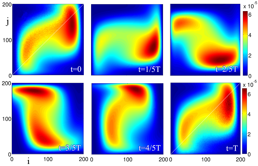
For $\omega=0.1$ size_issue , the stochastic simulations reveal a metastable state which is distinctively different from the limit cycle produced by the mean-field equations, see Fig. 3b. There is a conflict between the evolution of means, described by the adjusted replicator equations, and the results of the stochastic dynamics. The conflict can be resolved with the concept of the quasi-stationary distribution. Namely, the transition matrices, Eq. (1), are round-specific now and form a set $\{\tilde{\mathbf{S}}^{m}\}$, $m=1,\cdots,M$. The propagator over the time interval $[0,t]$, $0<t<T$, is the product $\tilde{\mathbf{U}}(t)=\prod_{m^{\prime}=1}^{M_{t}}\tilde{\mathbf{S}}^{m^{\prime}}$ with $M_{t}=t/\triangle t$. All the propagators, including the period-one propagator $\tilde{\mathbf{U}}(T)$, have the same structure as the super-matrix in Eq. (1). We define the metastable state $\mathbf{d}(T)$ as the the quasi-stationary distribution of $\tilde{\mathbf{U}}(T)$. It is also a Floquet state floquetH of the reduced propagator $\tilde{\mathbf{U}}^{r}(T)$, which can be obtained by replacing the transition matrices $\tilde{\mathbf{S}}^{m^{\prime}}$ with the matrices $\tilde{\mathbf{Q}}^{m^{\prime}}$ or by simply cutting out the first line and column from the matrix $\tilde{\mathbf{U}}(T)$. The Floquet state is a time-periodic state, $\mathbf{d}(t+T)=\mathbf{d}(t)$, which changes during one period of modulations, see Fig. 4. The metastable state $\mathbf{d}(t)$ at any instant of time $t$, $0<t<T$, can be obtained by acting on the state $\mathbf{d}(0)$ with the reduced propagator $\tilde{\mathbf{U}}^{r}(t)$.

Figure 3: (color online) Evolutionary dynamics governed by the BoS game with modulated payoffs. (a) Period-one limit cycles of the mean-field dynamics for $\omega=0.1$ (blue dash-dotted line) and $\omega=0.01$ (red solid line) are localized near the Nash equilibrium of the stationary game, $\left(\frac{1}{2},\frac{1}{2}\right)$ (arrows indicate the direction of motion). In the limit $\omega\rightarrow 0$, the mean-field attractor shrinks to the set of adiabatic Nash equlibria (black dashed line). Mean position ($\bullet$) of a finite-$N$ metastable Floquet state, $\left(\bar{x}(t),\bar{y}(t)\right)$, Eq. (2), moves along the limit cycle localized near the point $\left(\frac{1}{2},\frac{1}{2}\right)$ (the means are plotted at the instants $t_{n}=nT/5$, $n=0,..,4$); (b) A stochastic trajectory (grey line) reveals the existence of a period-two limit cycle [the period doubling can be resolved with stroboscopic points, plotted at the instants $2nT$ ($\bigtriangleup$) and $(2n+1)T$ ($\diamondsuit$)]. The trajectory is initiated at the point marked with the open blue square and ends up at the absorbing state (red cross at the upper left corner). The trajectory of the mean of the finite-$N$ metastable Floquet state ($\bullet$) is distinctively different from the stochastic trajectory [note the change of scale as compared to panel (a)]. The parameters are $f=0.5$, $N=200$, and $M=T/\triangle t=10N$ (corresponds to the driving frequency $\omega=0.1$ in the mean-field limit) size_issue . Other parameters as in Fig. 2.

The evolution of the means of the pdf $\mathbf{d}(t)$ (see Fig. 4a), $\left(\bar{x}(t),\bar{y}(t)\right)$, is close to the period-one limit cycle, see blue dots on Fig. 3a. However, the Floquet state consists of two peaks produced by the noised period-two limit cycle (compare also the positions of the stroboscopic points in Fig. 3b with the pdf for $t=0$ in Fig. 4a). The peak contributions balance each other thus reducing the dynamics of the means to the vicinity of the the point $\left(\frac{1}{2},\frac{1}{2}\right)$.

Figure 4: (color online) Evolution of the metastable Floquet state over one period of modulations. The pdfs obtained by the direct diagonalization of the reduced period-one propagator for $N=200$. The corresponding means $\left(\bar{x}(t),\bar{y}(t)\right)$ are shown on Fig. 3a ( $\bullet$). Plots for $t=0$ (above the diagonal) and $t=T$ (below the diagonal) present the results of the stochastic sampling.

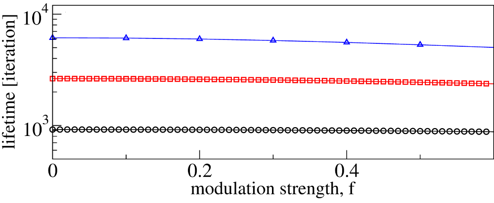
The lifetime of the state $\mathbf{d}(t)$ can be estimated with the largest eigenvalue $\lambda_{T}$, $0<\lambda_{T}<1$, of the matrix $\tilde{\mathbf{U}}^{r}(T)$. To compare it with lifetimes of stationary metastable states, we introduce the mean single-round exponent, $\bar{\lambda}_{T}=\lambda_{T}^{1/M}$ and define the mean lifetime as $t_{\mathrm{life}}=1/(1-\bar{\lambda}_{T})$ generic . Aside of the slow decay trend, we found the effect of modulations not being strong. This is in stark contrast to the structure of the metastable states. Namely, while in the stationary limit the pdf $\mathbf{d}$ is localized near the Nash equilibrium, at the maximal distance from the absorbing boundaries, the metastable Floquet state is localized near the absorbing boundary, see Fig. 4. We also detect the increase of the boundary localization with the increase of the population size beyond $N=200$. This suggests that, in the limit $N\rightarrow\infty$, the dynamics of the system is governed by a period-two limit cycle localized near the absorbing boundary. The boundary localization of the metastable attractor can be interpreted as the presence of small fractions of mutants smith , i.e. the players that are using strategies different from that used by the majority of populations. The evolutionary dynamics of the mutant fractions looks like a repeating sequence of population bottlenecks dawkins ; bottleneck yet this only weakly affects fraction lifetimes issue1 even in the case of finite $N$.

Conclusions. We presented a concept of metastable Floquet states in game-driven populations when mate selection preferences are periodically changing in time. Here we combined the Floquet formalism with the concept of quasi-stationary distributions to reveal the existence of complex, liquid-like nonequlibrium dynamics in the strategy space which cannot be resolved within the mean-field framework. Metastable Floquet states are not restricted to the field of ecology studies but can emerge in different periodically modulated systems with stochastic event-driven dynamics. They may, for example, underlay a gene expression in a single cell, which is modulated by a circadian rhythm cyrcadian and can provide new interpretations of the Bose-Einstein condensation in ac-driven atomic ensembles ketz ; frey2 .

I Seasonal variations in mate preferences

Stable time variations were found in the female flycatcher preferences or male forehead patch size that resulted in late-breeding females preferring males with larger patches fly . It was explained by the fact that in the beginning of the breeding season, large-patched males allocate more resources to courting than to parental care but change their habits to the opposite late in the season. Seasonal variations were also found in fiddle crabs (female preference to male claw size) crab , two-spotted goby (female preference to overall male size) goby , and sailfin mollies (male preferences for two different kind of females) molly .

II Moran process

Players $A$ (males) and $B$ (females) form two populations, each one of a fixed size $N$ and with two available strategies, $s=\{1,2\}$. Payoffs are specified by four functions, $\{a_{ss^{\prime}}(t)\}$ and $\{b_{s^{\prime}s}(t)\}$, $s,s^{\prime}=\{1,2\}$. The average payoff of the players using strategy $s$ is

$$~{}\pi^{A}_{s}(j,t)=a_{s1}(t)\frac{j}{N}+a_{s2}(t)\frac{(N-j)}{N},$$ (3)

$$\pi^{B}_{s}(i,t)=b_{s1}(t)\frac{i}{N}+b_{s2}(t)\frac{(N-i)}{N}.~{}$$ (4)

Payoffs determine the probabilities for a player to be chosen for reproduction, e.g. for the male population,

$$P^{A}_{s}(i,j,t)=\frac{1}{N}\cdot\frac{1-w+w\pi^{A}_{s}(j,t)}{1-w+w\bar{\pi}^{A}(i,j,t)},$$ (5)

where $\bar{\pi}^{A}(i,j,t)=[i\pi^{A}_{1}(j,t)+(N-i)\pi^{A}_{2}(j,t)]/N$ is the average payoff of the males. The baseline fitness $w\in[0,1]$ is a tunable baseline fitness parameter determining how the player’s chance to be chosen for reproduction is related to player’s performance moranNature ; traulsen1 . When $w=0$, the probability to be chosen for reproduction does not depend on player’s performance and is uniform across the population.

After the choice has been made, another member of the population is chosen completely randomly and replaced with an offspring of the player chosen for reproduction, i.e. with a player using the same strategy as its parent imitation . This update mechanism is acting simultaneously in both populations, $A$ and $B$, such that a mating pair produces two offspring, a male and a female, on every round. Therefore, the size of the populations $N$ remains constant.

A single round can be considered as a one-step Markov process, with transition rates, e.g. for population $A$, from a state $i$ to states $i+1$ and $i-1$, are given by traulsen1 ; traulsen4

$$T_{A}^{+}(i,j,t)=\frac{1-w+w\pi^{A}_{1}(t)}{1-w+w\bar{\pi}^{A}}\frac{i}{N}\frac{N-i}{N},$$

$$T_{A}^{-}(i,j,t)=\frac{1-w+w\pi^{A}_{2}(t)}{1-w+w\bar{\pi}^{A}}\frac{N-i}{N}\frac{i}{N}.$$ (6)

III Transition tensor

Here we describe the transition fourth-order tensor $S^{m}(i,j,i^{\prime},j^{\prime})$ in terms of the rates [$T_{A}^{+,-}(i,j,t)$ and $T_{B}^{+,-}(i,j,t)$] for populations $A$ and $B$ given by Eq. (4) in the main text. The stochastic Moran process can be expressed as a Markov chain traulsen4

$$p^{m+1}(i,j) = \left[1-T_{A}^{+}(i,j,m\triangle t)-T_{A}^{-}(i,j,m\triangle t)\right]\left[1-T_{B}^{+}(i,j,m\triangle t)-T_{B}^{-}(i,j,m\triangle t)\right]p^{m}(i,j)$$ (7)

$$+T_{B}^{-}(i,j+1,m\triangle t)\left[1-T_{A}^{-}(i,j+1,m\triangle t)-T_{A}^{+}(i,j+1,m\triangle t)\right]p^{m}(i,j+1)$$

$$+T_{B}^{+}(i,j-1,m\triangle t)\left[1-T_{A}^{-}(i,j-1,m\triangle t)-T_{A}^{+}(i,j-1,m\triangle t)\right]p^{m}(i,j-1)$$

$$+T_{A}^{-}(i+1,j,m\triangle t)\left[1-T_{B}^{-}(i+1,j,m\triangle t)-T_{B}^{+}(i+1,j,m\triangle t)\right]p^{m}(i+1,j)$$

$$+T_{A}^{+}(i-1,j,m\triangle t)\left[1-T_{B}^{-}(i-1,j,m\triangle t)-T_{B}^{+}(i-1,j,m\triangle t)\right]p^{m}(i-1,j)$$

$$+T_{A}^{-}(i+1,j+1,m\triangle t)T_{B}^{-}(i+1,j+1,m\triangle t)p^{m}(i+1,j+1)$$

$$+T_{A}^{+}(i-1,j+1,m\triangle t)T_{B}^{-}(i-1,j+1,m\triangle t)p^{m}(i-1,j+1)$$

$$+T_{A}^{-}(i+1,j-1,m\triangle t)T_{B}^{+}(i+1,j-1,m\triangle t)p^{m}(i+1,j-1)$$

$$+T_{A}^{+}(i-1,j-1,m\triangle t)T_{B}^{+}(i-1,j-1,m\triangle t)p^{m}(i-1,j-1).$$

The above equation can be recast into

$$p^{m+1}(i,j) = \sum_{i^{\prime},j^{\prime}}S^{m}(i,j,i^{\prime},j^{\prime})p^{m}(i^{\prime},j^{\prime}),$$ (8)

where the fourth-order tensor $S^{m}(i,j,i^{\prime},j^{\prime})$ is given by,

$$S^{m}(i,j,i^{\prime},j^{\prime}) = \left[1-T_{A}^{+}(i^{\prime},j^{\prime},m\triangle t)-T_{A}^{-}(i^{\prime},j^{\prime},m\triangle t)\right]\left[1-T_{B}^{+}(i^{\prime},j^{\prime},m\triangle t)-T_{B}^{-}(i^{\prime},j^{\prime},m\triangle t)\right]\delta_{i^{\prime},i}\,\delta_{j^{\prime},j}$$ (9)

$$+T_{B}^{-}(i^{\prime},j^{\prime},m\triangle t)\left[1-T_{A}^{-}(i^{\prime},j^{\prime},m\triangle t)-T_{A}^{+}(i^{\prime},j^{\prime},m\triangle t)\right]\delta_{i^{\prime},i}\,\delta_{j^{\prime},j+1}$$

$$+T_{B}^{+}(i^{\prime},j^{\prime},m\triangle t)\left[1-T_{A}^{-}(i^{\prime},j^{\prime},m\triangle t)-T_{A}^{+}(i^{\prime},j^{\prime},m\triangle t)\right]\delta_{i^{\prime},i}\,\delta_{j^{\prime},j-1}$$

$$+T_{A}^{-}(i^{\prime},j^{\prime},m\triangle t)\left[1-T_{B}^{-}(i^{\prime},j^{\prime},m\triangle t)-T_{B}^{+}(i^{\prime},j^{\prime},m\triangle t)\right]\delta_{i^{\prime},i+1}\,\delta_{j^{\prime},j}$$

$$+T_{A}^{+}(i^{\prime},j^{\prime},m\triangle t)\left[1-T_{B}^{-}(i^{\prime},j^{\prime},m\triangle t)-T_{B}^{+}(i^{\prime},j^{\prime},m\triangle t)\right]\delta_{i^{\prime},i-1}\,\delta_{j^{\prime},j}$$

$$+T_{A}^{-}(i^{\prime},j^{\prime},m\triangle t)T_{B}^{-}(i^{\prime},j^{\prime},m\triangle t)\delta_{i^{\prime},i+1}\,\delta_{j^{\prime},j+1}$$

$$+T_{A}^{+}(i^{\prime},j^{\prime},m\triangle t)T_{B}^{-}(i^{\prime},j^{\prime},m\triangle t)\delta_{i^{\prime},i-1}\,\delta_{j^{\prime},j+1}$$

$$+T_{A}^{-}(i^{\prime},j^{\prime},m\triangle t)T_{B}^{+}(i^{\prime},j^{\prime},m\triangle t)\delta_{i^{\prime},i+1}\,\delta_{j^{\prime},j-1}$$

$$+T_{A}^{+}(i^{\prime},j^{\prime},m\triangle t)T_{B}^{+}(i^{\prime},j^{\prime},m\triangle t)\delta_{i^{\prime},i-1}\,\delta_{j^{\prime},j-1}.$$

Above $i=0,\cdots,N$, $j=0,\cdots,N$, $i^{\prime}=0,\cdots,N$, and $j^{\prime}=0,\cdots,N$. Using the bijection $k=(N-1)j+i$ and $l=(N-1)j^{\prime}+i^{\prime}$, we obtain the required matrix form, see Eq. (7) in the main text.

IV Adjusted replicator equations

In the continuous limit $N\rightarrow\infty$, the dynamics of the variables $x=i/N$ and $y=j/N$ is defined by the adjusted replicator equations smith ; hof2 ,

$$\dot{x}=[1-x][\Delta^{A}(t)-\Sigma^{A}(t)y]\frac{1}{\Gamma+\bar{\pi}^{A}(x,y,t)},$$ (10)

$$\dot{y}=[1-y][\Delta^{B}(t)-\Sigma^{B}(t)x]\frac{1}{\Gamma+\bar{\pi}^{B}(x,y,t)},$$ (11)

where $\Delta^{C}=c_{12}-c_{22}$, $\Sigma^{C}=c_{11}+c_{22}-c_{12}-c_{21}$, $\Gamma=\frac{1-w}{w}$, and $C=\{A,B\}$. $\bar{\pi}^{A}(x,y,t)$ [$\bar{\pi}^{B}(x,y,t)$] is the averaged (over the population) payoff of the males [females].

V The lifetime of a metastable state

The lifetime of the state $\mathbf{d}(t)$ can be estimated with the largest eigenvalue $\lambda_{T}$, $0<\lambda_{T}<1$, of the matrix $\tilde{\mathbf{U}}^{r}(T)$. To compare it with lifetimes of stationary metastable states, we introduce the mean single-round exponent, $\bar{\lambda}_{T}=\lambda_{T}^{1/M}$ and define the mean lifetime as $t_{\mathrm{life}}=1/(1-\bar{\lambda}_{T})$. Figure 1 shows the dependence of $t_{\mathrm{life}}$ on the strength of modulations.

Figure 5: (color online) The lifetime $t_{\mathrm{life}}$ as a function of the modulation strength $f$, for the population size $N=50$ ($\bigcirc$), $100$ ($\Box$), and $200$ ($\triangle$). Other parameters are as in Fig. 2 in the main text.

VI Simulations

The preconditioned stochastic sampling was performed by launching trajectories from random initial points, uniformly distributed on the $N-1\times N-1$ grid and then sampling the pdf with only those trajectories which remained unabsorbed after $10\cdot N^{2}$ rounds.

For $N=200$ the diagonalization of the $39~{}601\times 39~{}601$ matrix $\tilde{\mathbf{Q}}_{T}$ was performed on the cluster of the MPIPKS (Dresden) and Leibniz-Rechenzentrum (München). The stochastic sampling was performed on a GPU cluster consisting of twelve TESLA K20XM cards. That allowed us to obtain $5\cdot 10^{8}$ realizations for each set of parameters.

References

- (1) M. Andersson, Sexual Selection(Princeton Univ. Press. Princeton, 1994).
- (2) R. Dawkins, The Selfish Gene (Oxford University Press, Oxford, 1976).
- (3) See Supplemental Material for more information.
- (4) D. Crews, Science 189, 1059 (1975).
- (5) M. M. Holmes, C. L. Bartrem, and J. Wade, Physiol. and Behav. 91, 601 (2007).
- (6) V. D. Jennions and M. Petrie, Biol. Rev. Cambridge Philos Soc., 72 (2006).
- (7) J. N. Darroch and E. Seneta, J. Appl. Prob. 2, 88 (1965).
- (8) G. Floquet, Annales de l’École Normale Supérieure 12, 47 (1883).
- (9) M. Grifoni and P. Hänggi, Phys. Rep. 304, 229 (1998).
- (10) G. Biroli and J. Kurchan, Phys. Rev. E 64, 016101 (2001).
- (11) S. Rulands, T. Reichenbach, and E. Frey, J. Stat. Mech. L01003 (2011).
- (12) M. Assaf and M. Mobilia, Phys. Rev. Lett. 109, 188701 (2012).
- (13) J. Hofbauer and K. H. Schlag, J. of Evol. Economics 10, 523 (2000).
- (14) K. H. Schlag, J. of Econom. Theory 78, 130.
- (15) A. Traulsen, J. C. Claussen, and C. Hauert, Phys. Rev. Lett. 95, 238701 (2005).
- (16) Ch. S. Gokhale and A. Traulsen, Dyn. Games and Appl. 4, 468 (2014).
- (17) A. Traulsen, J. C. Claussen, and C. Hauert, Phys. Rev. E. 74, 011901 (2006).
- (18) A. Dobrinevski and E. Frey, Phys. Rev. E 85, 051903 (2012).
- (19) P. A. P. Moran, The Statistical Processes of Evolutionary Theory (Clarendon, Oxford, 1962).
- (20) M. A. Nowak, A. Sasaki, C. Taylor, and D. Fudenberg, Nature 428, 646 (2004).
- (21) J. M. Smith, Evolution and the Theory of Games(Cambridge University Press, Cambridge, 1982).
- (22) E. Seneta, Non-negative Matrices and Markov Chains (Springer, NY, 2006).
- (23) M. Khasin and M. I. Dykman, Phys. Rev. Lett. 103, 068101 (2009).
- (24) By virtue of the Perron-Frobenius theorem, and are both real and non-negative gant .
- (25) This choice corresponds to the Matching Pennies game, see J. von Neumann and O. Morgenstern, Theory of Games and Economic Behaviour (Princeton University Press, Princeton, 1944).
- (26) J. Nash, PNAS 36, 48 (1950).
- (27) A. Trauslen, J. C. Claussen, and C. Hauert, Phys. Rev. E 85, 041901 (2012).
- (28) L. Arnold, Random Dynamical Systems (Springer, NY, 2003).
- (29) P. J. Thomas and B. Lindner, Phys. Rev. Lett. 113, 254101 (2014).
- (30) A. J. Black, A. Traulsen, and T. Galla, Phys. Rev. Lett. 109, 028101 (2012).
- (31) The average absorption time for a specific initial state, , is proportional the corresponding entry in the left maximal-eigenvalue eigenvector of the reduced matrix . The proportionality coefficient can be found from the dual orthonormality condition.
- (32) We find a sharp contrast between the mean-filed dynamics and the stochastic evolution for this particular value of . The optimal value for the frequency (period) of modulations could be different for other driving scheme and/or other choice of the game payoffs.
- (33) T. Maruyama and P. A. Fuerst, Genetics 111, 691 (1985).
- (34) The relations between the exponent , mean absorption (fixation) time meantime , and dynamical properties of Floquet states is an interesting issue. It can be explored, for example, with a discrete-time generalization of the “optimal path to exctintion” approach dykman2 ; escudero ; meerson .
- (35) M. I. Dykman, E. Mori, J. Ross, and P. M. Hunt, J. Chem. Phys. 100, 5735 (1994).
- (36) C. Escudero and J. A. Rodriguez, Phys. Rev. E 77, 011130 (2008).
- (37) M. Assaf, A. Kamenev, and B. Meerson, Phys. Rev. E 78, 041123 (2008).
- (38) S. S. Golden, V. M. Cassone, and A. Li Wang, Nat. Struct. Mol. Biol. 14, 362 (2007); A. Sancar, Nat. Struct. Mol. Biol. 15, 23 (2008).
- (39) D. Vorberg, W. Wustmann, R. Ketzmerick, and A. Eckardt, Phys. Rev. Lett. 111, 240405 (2013).
- (40) J. Knebel, M. F. Weber, T. Krüger, and E. Frey, Nature Comm. 6, 6977 (2015).
Supplemental Material
- (1) A. Qvarnström, T. Pärt, and B. C. Sheldon, Nature 405, 344 (2000).
- (2) R. N. C. Milner, et al., Behav. Ecology 21, 311(2010).
- (3) A. A. Borg, E. Forsgren, and T. Amudsen, Anim. Behav. 72, 763 (2006).
- (4) K. U. Heubel and J. Schlupp, Behav. Ecol. 19, 1080 (2008).
- (5) M. A. Nowak, A. Sasaki, C. Taylor, and D. Fudenberg, Nature 428, 646 (2004).
- (6) A. Traulsen, J. C. Claussen, and C. Hauert, Phys. Rev. Lett. 95, 238701 (2005).
- (7) These two consecutive steps, death and birth, can be reinterpreted as a single step of imitation, i.e. adoption of the strategy of the first player by the second one hof2 ; schlag .
- (8) J. Hofbauer and K. H. Schlag, J. of Evol. Economics 10, 523 (2000).
- (9) K. H. Schlag, J. of Econom. Theory 78, 130.
- (10) A. Trauslen, J. C. Claussen, and C. Hauert, Phys. Rev. E 85, 041901 (2012).
- (11) J. M. Smith, Evolution and the Theory of Games(Cambridge University Press, Cambridge, 1982).