Prospects for measuring the Higgs coupling to light quarks

Abstract

Abstract

We discuss the prospects to probe the light-quark Yukawa couplings to the Higgs boson. The Higgs coupling to the charm quark can be probed both via inclusive and exclusive approaches. On the inclusive frontier, we use our recently proposed method together with published experimental studies for the sensitivity of the Higgs coupling to bottom quarks to find that the high-luminosity LHC can be sensitive to modifications of the charm Yukawa of the order of a few times its standard model (SM) value. We also present a preliminary study of this mode for a $100$ TeV hadronic machine (with similar luminosity) and find that the bound can be further improved, possibly within the reach of the expected signal in the SM. On the exclusive frontier, we use the recent ATLAS search for charmonia and photon final state. This study yields the first measurement of the background relevant to these modes. Using this background measurement we project that at the high-luminosity LHC, unless the analysis strategy is changed, the sensitivity of the exclusive final state to the charm Yukawa to the charm Yukawa will be rather poor, of the order of $50$ times the SM coupling. We then use a Monte-Carlo study to rescale the above backgrounds to the $h\to\phi\gamma$ case and obtain a much weaker sensitivity to the strange Yukawa, of order of $3000$ times the SM value. We briefly speculate what would be required to improve the prospects of the exclusive modes.

1 Introduction

Now that the Higgs particle has been discovered Aad et al. (2012); Chatrchyan et al. (2012) the standard model (SM) is complete. It has a minimal scalar sector of electroweak (EW) symmetry breaking and is a theory consistent up to very high scales. Furthermore, the SM enjoys a set of accidental (exact and approximate) symmetries leading to: baryon$-$lepton number conservation, suppression of processes involving flavor-changing neutral currents and CP violation. Nevertheless, the flavor sector of the SM has a very particular structure. The Higgs couplings depend linearly on the masses, which implies that most of the Yukawas are small and hierarchical, leading to the SM flavor puzzle. However, at present there is no strong direct evidence for the validity of this particular structure. For instance, it is not impossible that the masses of the first two generation fermions originate from a different source of EW symmetry breaking thus leading to deviations from the simple SM relation between fermion masses and their coupling to the Higgs.

With new physics it is actually easy to obtain enhancements or suppressions in the strengths of Higgs to light-quark interactions. Furthermore, as the Higgs is rather light, within the SM it can only decay to particles that interact very weakly with it, with the dominant decay to $b\bar{b}$. A deformation of the Higgs couplings to the lighter SM particles, say for the charm or other quarks (see Refs. Delaunay et al. (2013, 2014a); Blanke et al. (2013); Mahbubani et al. (2013); Kagan et al. (2009); Dery et al. (2013); Giudice and Lebedev (2008); Da Rold et al. (2013); Dery et al. (2014); Bishara et al. (2015)), could compete with the Higgs–bottom coupling and would lead to a dramatic change of the Higgs phenomenology Delaunay et al. (2014b).

Our knowledge of the Higgs Yukawa couplings is mainly on the third-generation charged fermions. Though not yet fully conclusive, it is consistent with the SM Higgs mechanism of fermion-mass generation The ATLAS Collaboration, ATLAS-CONF-2014-011, ATLAS-COM-CONF-2014- (004); Aad et al. (2014a, 2015a); Khachatryan et al. (2014a); Chatrchyan et al. (2014a, b). Regarding the first two generations, at present, we only have a rather weak upper bound on the corresponding signal strengths of muons and electrons Aad et al. (2014b); Khachatryan et al. (2014b)

$$\mu_{\mu}\leq 7\,,\quad\quad\mu_{e}\leq 4\times 10^{5}\,,$$ (1)

at 95% Confidence Level (CL) where $\mu_{f}\equiv\frac{\sigma_{h}}{\sigma_{h}^{\rm SM}}\,\frac{{\rm BR}_{f\bar{f}}}{{\rm BR}_{f\bar{f}}^{\rm SM}}$ with $\sigma_{h}$ standing for the Higgs-production cross section, ${\rm BR}_{X}\equiv{\rm BR}(h\to X)$ and the SM script indicating the SM case. In addition, in Ref. Perez et al. (2015) we recasted the ATLAS Aad et al. (2014a) and CMS Chatrchyan et al. (2014a) studies of $Vh(b\bar{b})$ and obtained a first direct bound on the charm signal strength,

$$\mu_{c}\leq 270\,,$$ (2)

at $95$% CL. These bounds are very weak, yet they are sufficient to exclude Higgs-coupling universality to quarks and charged leptons.

Let us summarise the current status of the theoretical and experimental activity relevant to probing Higgs to light-quark couplings. On the theoretical frontier, it was demonstrated in Refs. Delaunay et al. (2014b); Perez et al. (2015) that inclusive charm-tagging enables the LHC experiments to constrain the charm Yukawa coupling. Furthermore, it was shown that the Higgs–charm coupling may be probed by looking at exclusive decay modes involving a $c$-$\bar{c}$ vector meson and a photon Bodwin et al. (2013). This makes the charm Yukawa coupling rather special among the light quarks as it can be probed both with inclusive and exclusive approaches. A similar mechanism, based on exclusive decays to light-quark states and gauge bosons $\gamma/W/Z$, was shown to yield a potential access to the Higgs–light-quark couplings Kagan et al. (2014). (See also Refs. Isidori et al. (2014); Mangano and Melia (2014); Huang and Petriello (2014); Grossmann et al. (2015) for studies of exclusive EW gauge-boson decays and new-physics searches.) On the experimental side, ATLAS recently published two searches for supersymmetry Aad et al. (2014c, 2015b), which employ charm-tagging ($c$-tagging) ATL (2015). ATLAS further published an analysis that focuses on Higgs decays to quarkonia (e.g. $J/\psi$, $\Upsilon$) plus a photon final states Aad et al. (2015c).

In this paper, we discuss the prospects to probe light-quark Yukawa couplings to the Higgs boson at LHC run II, the high-luminosity LHC (HL-LHC) and possible future colliders. We will demonstrate that the HL-LHC can reach a sensitivity for the charm Yukawa up to few times the SM value by using the inclusive method recently proposed by us Perez et al. (2015). We also present a preliminary study of this mode for a $100$ TeV hadronic machine assuming similar luminosity as at the HL-LHC. We shall find that the sensitivity can be further improved, possibly probing the signal expected in the SM. On the exclusive frontier we shall use the recent ATLAS result on the search for charmonia plus a photon final state Aad et al. (2015c). This study yields the first measurement of the background relevant to these modes. It is dominated by a jet converted to photon or a real photon plus charmonia production. Given this background measurement, we project that, unless the analysis strategy is changed, the sensitivity of the exclusive final state to the charm Yukawa at the HL-LHC will be rather poor, of the order of $50$ times the SM coupling. We then use a PYTHIA simulation to rescale the above backgrounds to the $h\to\phi\gamma$ case and obtain a much weaker sensitivity to the strange Yukawa of order of $3000$ times the SM value.

In the following section we discuss the prospects for probing the charm Yukawa coupling using charm tagging. In Section 3 we focus on the exclusive case. For completeness, we also briefly describe in Section 2.3 the corresponding status for $e^{+}e^{-}$ machines. We conclude in Section 4.

2 Inclusive Analysis

We begin by estimating the future sensitivity of the LHC and a future $100$ TeV $pp$ collider to probe the $h\to{c\bar{c}}$ signal strength, $\mu_{c}$, and the charm Yukawa, $\kappa_{c}\equiv y_{c}/y^{\rm SM}_{c}$, via the inclusive method proposed in Ref. Perez et al. (2015). The method takes advantage of the fact that the signal strength in searches for $h\to b\bar{b}$ requires two $b$-tagged jets. In this way, the same analyses are also sensitive to $h\to{c\bar{c}}$ events because charm jets ($c$-jets) pass the tag criteria with a non-negligible rate. To account for such events, the $h\to b\bar{b}$ signal strength, $\mu_{b}$, is extended

$$\mu_{b}\equiv\frac{\sigma_{h}{\rm BR}_{{b\bar{b}}}}{\sigma^{\rm SM}_{h}{\rm BR}_{{b\bar{b}}}^{\rm SM}}\,\to\,\frac{\sigma_{h}{\rm BR}_{{b\bar{b}}}\epsilon_{b_{1}}\epsilon_{b_{2}}+\sigma_{h}{\rm BR}_{{c\bar{c}}}\epsilon_{c_{1}}\epsilon_{c_{2}}}{\sigma^{\rm SM}_{h}{\rm BR}_{{b\bar{b}}}^{\rm SM}\epsilon_{b_{1}}\epsilon_{b_{2}}+\sigma^{\rm SM}_{h}{\rm BR}_{{c\bar{c}}}^{\rm SM}\epsilon_{c_{1}}\epsilon_{c_{2}}}=\left(\mu_{b}+\frac{{\rm BR}_{{c\bar{c}}}^{\rm SM}}{{\rm BR}_{{b\bar{b}}}^{\rm SM}}\frac{\epsilon_{c_{1}}\epsilon_{c_{2}}}{\epsilon_{b_{1}}\epsilon_{b_{2}}}\mu_{c}\right)\Bigg{/}\left(1+\frac{{\rm BR}_{{c\bar{c}}}^{\rm SM}}{{\rm BR}_{{b\bar{b}}}^{\rm SM}}\frac{\epsilon_{c_{1}}\epsilon_{c_{2}}}{\epsilon_{b_{1}}\epsilon_{b_{2}}}\right)\,.$$ (3)

Here, $\epsilon_{b}$ and $\epsilon_{c}$ are the efficiencies to tag jets originating from bottom and charm quarks, respectively. The subscripts $1$ and $2$ refer to the efficiency of tagging the first and second jet, respectively and ${\rm BR}_{{c\bar{c}}}^{\rm SM}/{\rm BR}_{{b\bar{b}}}^{\rm SM}\simeq 5\%$ Heinemeyer et al. (2013). For brevity, we define the ratio of tagging efficiencies, $\epsilon_{c/b}^{2}\equiv(\epsilon_{c_{1}}\epsilon_{c_{2}})/(\epsilon_{b_{1}}\epsilon_{b_{2}})$.

An analysis employing a single jet-tagger, such as medium $b$-tagging, constrains only a linear combination of $\mu_{b}$ and $\mu_{c}\,$. To be able to separately obtain $\mu_{c}$ we need at least two analyses with different ratios, $\epsilon_{c/b}^{2}$, in order to break the degeneracy in Eq. (3). The sensitivity is best when in the employed tagger $\epsilon_{c/b}^{2}$ is large meaning that many $c$-jets are being tagged. This situation is realized if we combine $b$-tagging with charm tagging ($c$-tagging), which is a jet-tagger optimized for $c$-jets. For the $b$-tagger we will always consider the medium $b$-tagging working point as in Ref. The ATLAS Collaboration, ATL-PHYS-PUB-2014-011 . For $c$-tagging we shall use what ATLAS already employed at run I Aad et al. (2014c, 2015b); ATL (2015) and refer to it as $c$-tagging I. Moreover, given the recent installation of the new Insertable B-Layer (IBL) subdetector Capeans et al. (2010) in the ATLAS detector, the capability for $c$-tagging is expected to be much improved. Related to this, Ref. ATLAS Collaboration shows possible improvement of the life-time resolution of $B^{0}_{s}\to J/\psi\,\phi$ decay by 30%, thanks to the IBL. Thus, we consider two additional $c$-taggings, referred to as $c$-tagging II and $c$-tagging III. All tagging efficiencies are summarized in Table 1 in which $\epsilon_{l}$ denotes the efficiency to tag a light jet.

	$\bm{\epsilon_{b}}$	$\bm{\epsilon_{c}}$	$\bm{\epsilon_{l}}$
$b$-tagging	$70\%$	$20\%$	$1.25\%$
$c$-tagging I	$13\%$	$19\%$	$0.5\%$
$c$-tagging II	$20\%$	$30\%$	$0.5\%$
$c$-tagging III	$20\%$	$50\%$	$0.5\%$

Table 1: The tagging efficiencies for the four jet-taggers used in our analysis.

$c$-tagging uses almost the same experimental information as $b$-tagging. As a result jets that are $c$-tagged may but also may not pass the $b$-tagging criteria ATL (2015); Chatrchyan et al. (2013). The actual experiments can employ $b$- and $c$-tagging simultaneously, but for our analysis it is not possible to fully take into account this correlation. Therefore, whenever possible, we study the following two extreme scenarios.

Uncorrelated scenario

$b$- and $c$-tagging are uncorrelated and possible to employ simultaneously. In this case, if a jet is $b$-tagged, the jet is never $c$-tagged, and vice versa, i.e., there is no overlap between $b$- and $c$-tagged jets.

Correlated scenario

$c$-tagging is fully correlated with $b$-tagging and is a tighter version of $b$-tagging. In this case, $c$-tagged jets are always also $b$-tagged, but the opposite is not necessary, i.e., $c$-tagged jets are a subset of $b$-tagged jets.

The actual situation is expected to be something between the following two scenarios. However, we will show in Section 2.1 that the final results in the two scenarios are similar. We define three categories by combining taggers: (i) two jets are $b$-tagged, (ii) one is $b$-tagged and one is $c$-tagged, (iii) two jets are $c$-tagged. To avoid double counting in categories (i) and (ii) of the correlated scenario, the $c$-tagged jets are removed from $b$-tagged jets. A schematic picture of the three categories for the scenarios is shown in Fig. 1. In our analysis we use RunDec Chetyrkin et al. (2000) to compute the quark masses at the Higgs mass using the inputs from PDG Olive et al. (2014) finding $m_{s}=53.2\,$MeV, $m_{c}=0.612\,$GeV and $m_{b}=2.78$  GeV.

Figure 1: Uncorrelated and correlated scenario in the left and right panel, respectively. $c$-tagged jets are a subset of $b$-tagged jets in the correlated scenario, while in the uncorrelated scenario $b$- and $c$-tagging cover different jets.

2.1 LHC 14 TeV

For LHC run II and HL-LHC, we base our study on the dedicated ATLAS analysis for the future measurement of $\mu_{b}$ based on the Higgs production associated with $W/Z$ bosons at LHC $14$ TeV with $300\,{\rm fb}^{-1}$ and $3000\,{\rm fb}^{-1}$ The ATLAS Collaboration, ATL-PHYS-PUB-2014-011 . The analysis requires two $b$-tagged jets, i.e., it employs a single tagger, which is insufficient to disentangle $\mu_{b}$ and $\mu_{c}$. To discuss the future sensitivities, we thus need to estimate the number of signal and background events in the three categories for the correlated and uncorrelated scenario once also $c$-tagging is employed. We utilize the Monte-Carlo (MC) studies presented in Figs. 3–6 of Ref. The ATLAS Collaboration, ATL-PHYS-PUB-2014-011 in the following way. These figures provide the number of events in each bin for signal and for each background after applying all cuts and requiring two $b$-tagged jets. Let us consider a bin of signal or a specific background that originally has an $x$- and a $y$-jet, where $x,y=b,c,l$ (real $b$-jet, $c$-jet, light-jet), and the number provided is $N$. We then obtain the number of events for categories (i)–(iii) in uncorrelated and correlated scenarios as below.

Uncorrelated scenario:

$$N^{\rm(i)}=N, N^{\rm(ii)}=\frac{\epsilon_{x}^{\text{($b$-tag)}}\epsilon_{y}^{\text{($c$-tag)}}+\epsilon_{x}^{\text{($c$-tag)}}\epsilon_{y}^{\text{($b$-tag)}}}{\epsilon_{x}^{\text{($b$-tag)}}\epsilon_{y}^{\text{($b$-tag)}}}N, N^{\rm(iii)}=\frac{\epsilon_{x}^{\text{($c$-tag)}}\epsilon_{y}^{\text{($c$-tag)}}}{\epsilon_{x}^{\text{($b$-tag)}}\epsilon_{y}^{\text{($b$-tag)}}}N\,,$$ (5)

Correlated scenario:

$$N^{\rm(i)}=N-N^{\rm(ii)}-N^{\rm(iii)}, N^{\rm(ii)}=\frac{\epsilon_{x}^{\text{($b$-tag)}}\epsilon_{y}^{\text{($c$-tag)}}+\epsilon_{x}^{\text{($c$-tag)}}\epsilon_{y}^{\text{($b$-tag)}}}{\epsilon_{x}^{\text{($b$-tag)}}\epsilon_{y}^{\text{($b$-tag)}}}N-2N^{\rm(iii)}, N^{\rm(iii)}=\frac{\epsilon_{x}^{\text{($c$-tag)}}\epsilon_{y}^{\text{($c$-tag)}}}{\epsilon_{x}^{\text{($b$-tag)}}\epsilon_{y}^{\text{($b$-tag)}}}N\,.$$ (6)

The rescaling is done on a bin-by-bin basis. After rescaling different background differently ($N\to B_{X}$ with $X$ denoting the type of background), we obtain the total background for each category, $B^{\rm(i,ii,iii)}$, by summing all backgrounds, $B^{\rm(i)}=\sum_{X}^{\text{all}}B_{X}^{\rm(i)}$ and analogously for (ii) and (iii). The expected signal for each category is straightforward, $N\to S$.

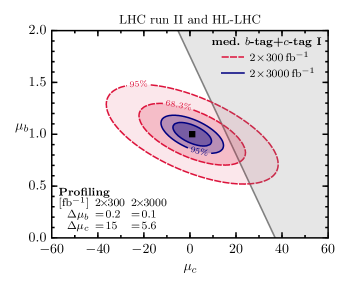
Figure 2: $300$ fb^-1 and $3000$ fb^-1 prospects for the signal strengths at the LHC, for $h\to b\bar{b}$ and $h\to c\bar{c}$ based on $b$- and $c$-tagging for the uncorrelated scenario employing $c$-tagging I (left panel) and $c$-tagging II (right panel). The grey shaded region is unphysical unless Higgs production is modified with respect to the SM case. The profiled likelihood ratio Cowan et al. (2011) is used for the respective 1-$\sigma$ uncertainty of $\Delta\mu_{b}$ and $\Delta\mu_{c}$.

To obtain the future sensitivity we then follow the statistical procedure described in Ref. Perez et al. (2015). Given the expectation of signal and background, we construct a likelihood function of $\mu_{c}$ and $\mu_{b}$ based on the Poisson probability-distribution function, and use the likelihood ratio for parameter estimates. In Fig. 2 we present the future reach for the signal strengths of $h\to b\bar{b}$ and $h\to c\bar{c}$ in the uncorrelated scenario by combining $b$-tagging with $c$-tagging I (left panel) and II (right panel). Note that the correlated scenario cannot be defined in the case of $c$-tagging II and III, see Appendix A for details and Fig. 6 therein for the $c$-tagging I result of the correlated scenario. We obtain the expected uncertainty on $\mu_{c}$ ($\mu_{b}$) by profiling $\mu_{b}$ ($\mu_{c}$). We list the $1$-$\sigma$ ranges for $\mu_{c}$ and $\mu_{b}$ for different scenarios and employed $c$-tagging assuming the total luminosity of $2\times 300$ fb^-1 and $2\times 3000$ fb^-1 expected at LHC run II and HL-LHC in Tab. 2. The sensitivities for $c$-tagging I in the correlated and uncorrelated scenario are similar, so we conclude that these results represent well the actual future reach.

$\cal L$	$\sqrt{s}=14$ TeV	$\Delta\mu_{b}$	$\Delta\mu_{c}$	$\Delta\kappa_{b}$	$\Delta\kappa_{c}$	$\kappa_{b}$ @ $95\%$ CL	$|\kappa_{c}|$ @ $95\%$ CL
$2\times 300$ fb-1	correlated $c$-tagging I	$\pm 0.22$	$\pm 15$	$+1.3$	$+8.6$	$[0.67,7.07]$	$<37$
	uncorrelated $c$-tagging I	$\pm 0.20$	$\pm 15$	$+1.5$	$+9.4$	$[0.69,7.16]$	$<38$
	uncorrelated $c$-tagging II	$\pm 0.18$	$\pm 10$	$+0.5$	$+4.1$	$[0.70,4.70]$	$<21$
	uncorrelated $c$-tagging III	$\pm 0.17$	$\pm 5.8$	$+0.29$	$+2.2$	$[0.70,1.90]$	$<6.0$
$2\times 3000$ fb-1	correlated $c$-tagging I	$\pm 0.084$	$\pm 5.6$	$+0.20$	$+2.1$	$[0.84,1.57]$	$<5.5$
	uncorrelated $c$-tagging I	$\pm 0.075$	$\pm 5.6$	$+0.20$	$+2.1$	$[0.85,1.60]$	$<5.6$
	uncorrelated $c$-tagging II	$\pm 0.069$	$\pm 3.7$	$+0.12$	$+1.4$	$[0.86,1.30]$	$<3.7$
	uncorrelated $c$-tagging III	$\pm 0.065$	$\pm 2.0$	$+0.087$	$+0.82$	$[0.87,1.18]$	$<2.5$

Table 2: $1$-$\sigma$ uncertainties after profiling Cowan et al. (2011) for the signal strengths, $\mu_{b}$ and $\mu_{c}$, and the Yukawa-coupling modifications, $\kappa_{b}$ and $\kappa_{c}$ at the LHC with $\sqrt{s}=14$ TeV. The results for different scenarios (uncorrelated and correlated) and different $c$-tagging are shown for a total luminosity of $2\times 300$ fb^-1 and $2\times 3000$ fb^-1. The error in $\kappa_{b}$ and $\kappa_{c}$ is asymmetric; we only show the upper bound. The $95\%$ CL regions for $\kappa_{b}$ and $\kappa_{c}$ are given in the last two columns.

The translation of the constraints of the charm and bottom signal strengths to the Yukawa couplings themselves requires some caution. If we assume that Higgs production is not modified with respect to the SM, the signal strengths are given by $\mu_{c}={\rm BR}_{c\bar{c}}/{\rm BR}^{\rm SM}_{c\bar{c}}$ and $\mu_{b}={\rm BR}_{b\bar{b}}/{\rm BR}^{\rm SM}_{b\bar{b}}$. In the extreme case in which the Higgs decays solely to charms and bottoms, ${\rm BR}_{c\bar{c}}+{\rm BR}_{b\bar{b}}=1\,$ holds and the two rates are linearly dependent. As long as the measured values of $\mu_{c}$ and $\mu_{b}$ are consistent with this hypothesis, an arbitrary large value of $\kappa_{c}\equiv y_{c}/y_{c}^{\rm SM}$ is allowed with some $\kappa_{b}\equiv y_{b}/y_{b}^{\rm SM}$. This corresponds to a flat direction in the $\kappa_{c}$–$\kappa_{b}$ plane. In other words, as long as the experimental result is consistent with

$$\mu_{c}{\rm BR}^{\rm SM}_{c\bar{c}}+\mu_{b}{\rm BR}^{\rm SM}_{b\bar{b}}>1\,,$$ (7)

one cannot constrain $\kappa_{c}$ and $\kappa_{b}$ assuming only SM Higgs production. We illustrate this case with the grey shaded region in Fig. 2. If this region overlaps with the allowed regions of $\mu_{c}$–$\mu_{b}$ (coloured ellipses), it means that there is a flat direction in the $\kappa_{c}$–$\kappa_{b}$ if SM Higgs production is assumed.

A charm Yukawa much larger than in the SM enhances the Higgs production in the $Vh$ production channel; for $\kappa_{c}\!\sim\!\mathcal{O}(100)$ it is twice as large as the SM expectation Perez et al. (2015). This mechanism enabled us to obtain a direct constraint on $\kappa_{c}$ already with the available $8$ TeV dataset Perez et al. (2015). For the $14$ TeV projection, as seen in Fig. 2, considering non-SM production is essential to constrain $\kappa_{c}$ with $300\,{\rm fb}^{-1}$, while for the high-luminosity stage its effect is minor. Details of non-SM $Vh$ production at 14  TeV are discussed in Appendix A.

In the analysis for the prospects for couplings, we float only $\kappa_{b}$ and $\kappa_{c}$ freely and assume the other couplings stay as in the SM, in particular, $\kappa_{V}=1$. In Fig. 3 we show the expected future reach in the $\kappa_{c}$–$\kappa_{b}$ plane taking into account non-SM $Vh$ production for the uncorrelated scenario employing $c$-tagging I and II. We obtain the expected upper bound on $\kappa_{c}$ ($\kappa_{b}$) by profiling over $\kappa_{b}$ ($\kappa_{c})$ Cowan et al. (2011). The $1$-$\sigma$ uncertainties, as well as the $95\%$ CL ranges for $\kappa_{b}$ and $\kappa_{c}$ for the different cases are listed in Tab. 2.

Finally, we compare the projected reach of the direct charm-Yukawa measurement to the indirect bound from the global analysis of the Higgs couplings. For $\kappa_{c}<5$ the effects of non-SM Higgs production due to large charm Yukawa are negligible and the constraint on $\kappa_{c}$ can be deduced from the bound on the untagged Higgs decays. The ATLAS projection for the HL-LHC is ${\rm BR}_{\rm untagged}<10\,\%$ at $95\%$ CL (without theoretical uncertainties) ATL (2014). It can be interpreted as $\kappa_{c}\lesssim 2\,$. This upper bound is comparable to our projection with $c$-tagging III, see Tab. 3.

Figure 3: $300$ fb^-1 and $3000$ fb^-1 prospects for probing $\kappa_{b}$ and $\kappa_{c}$ at the LHC, with $h\to b\bar{b}$ and $h\to c\bar{c}$ based on $b$- and $c$-tagging for the uncorrelated scenario employing $c$-tagging I (left panel) and $c$-tagging II (right panel). All other Higgs couplings are assumed to be like in the SM. The profiled likelihood ratio Cowan et al. (2011) is used for the respective reach on $\kappa_{b}$ and $\kappa_{c}$.

2.2 $pp$ collider with $\sqrt{s}=100$ TeV

In this section we perform a first study of the sensitivity reach of a $100$ TeV $pp$ collider in measuring the charm-quark Yukawa via the inclusive rate. As a byproduct we obtain also the sensitivity of a bottom-Yukawa measurement at $100$ TeV. For such a machine, there exists no detailed, fully realistic study for the $h\to b\bar{b}$ prospects like the one of ATLAS for $14$ TeV The ATLAS Collaboration, ATL-PHYS-PUB-2014-011 , which we employed for our $14$ TeV study. For this reason, we investigate the $100$ TeV reach by simulating the signal and main backgrounds at the leading-order (LO) parton level using MadGraph 5.2 Alwall et al. (2011) and multiplying with the inclusive $k$-factors.

The main difficulty remains to find a way to reduce background, while keeping as many signal $h\to c\bar{c}$ events as possible. To this end, we follow two orthogonal directions. Firstly, we look into the boosted-Higgs regime in which the Higgs has $p_{T}(h)>350$ GeV. In this case we rely on available jet-substructure techniques to extract the signal and reduce the $t\bar{t}$ background that dominates in this kinematic configuration. Secondly, we “unboost” the Higgs by binning in $H_{T}$. This way the $S/B$ ratio for $h\to c\bar{c}$ is large in lower $H_{T}$ bins as the main background, $t\bar{t}$, typically has higher $H_{T}$ than the signal.

We shall find that the sensitivity reach for the bottom Yukawa is not significantly different in the two cases, as in both there are enough $h\to b\bar{b}$ events. For the charm Yukawa, however, the “unboosted” analysis appears more promising, due to the fact that it accepts a larger fraction of the rather rare signal events. Given that the capabilities of a future $100$ TeV collider and the advancements with respect to current experiments are currently not well known, the fact that our projections will be based on LO simulations suffices. However, it is important to note that we expect significantly better results from realistic studies that employ multiple bins with increased $S/B$ ratio. For instance, the projected uncertainty on $\Delta\mu_{b}$ from Ref. The ATLAS Collaboration, ATL-PHYS-PUB-2014-011 would be approximately a factor of $2$ larger without binning. Furthermore, in Ref. The ATLAS Collaboration, ATL-PHYS-PUB-2014-011 the sensitivity of a purely cut-based analysis was compared to the one obtained employing multivariate techniques. In the latter the uncertainty is decreased by roughly $25\%$. This gives us confidence that the results presented here are conservative and there is room for improvements in the future.

Boosted-Higgs analysis

The field of searching for boosted massive particles and jet-substructure is very rich and we shall not attempt to describe it here in any detail (see e.g. Altheimer et al. (2014) for a recent review). Instead we focus on one specific method to study the sensitivity to the Higgs couplings to bottom and charm quarks at a $100$ TeV collider. The sensitivity to the $h\to b\bar{b}$ decay mode with the Higgs being boosted and produced in association with a leptonically decaying $W$ at the LHC with $\sqrt{s}=8$ and $13$ TeV has been analysed in Ref. Backovic et al. (2013). The study adopted the Template Overlap Method Almeida et al. (2010, 2012) (see also Aad et al. (2013) for the ATLAS implementation of the method). For our study we will use the signal efficiency and background-rejection rates of the “Cuts 5” scenario in Ref. Backovic et al. (2013) and a cut on the fat jet containing the Higgs (or its $b\bar{b}$ daughter products), $p_{T}(h)>350$ GeV. Given the above requirements, the $Wh$ signal has an efficiency of $22\%$ while the $t\bar{t}$ and $Wb\bar{b}$ backgrounds have a fake rate of only $1.3\%$ and $5.1\%$, respectively (see Tab. III in Ref. Backovic et al. (2013)). We will assume that these jet-substructure efficiencies do not change from $13$ to $100$ TeV.

Figure 4: Prospects for probing $\mu_{b}$, $\mu_{c}$ (left panel), and $\kappa_{b}$, $\kappa_{c}$ (right panel) at a $100$ TeV collider, with $h\to b\bar{b}$ and $h\to c\bar{c}$ based on $b$- and $c$-tagging II for the uncorrelated scenario using boosted Higgses and $2\times 3000$ fb^-1 of data. The profiled likelihood ratio Cowan et al. (2011) is used for the respective reach of $\Delta\mu_{b}$, $\Delta\mu_{c}$, $\kappa_{b}$, and $\kappa_{c}$.

To make use of these jet-substructure results for our $100$ TeV study we follow their analysis and simulate signal and background for both $13$ and $100$ TeV applying the same basic cuts. The main requirement is the presence of two $b$-tagged jets inside the fat jet and a few basic cuts the most relevant of which are $p_{T}(W),p_{T}({\text{fat jet}})>350$ GeV and $0.4<\Delta R_{bb}<0.8$ (see Eq. (12) and (13) in Ref. Backovic et al. (2013)). Their simulation of the signal $Wh$, and the backgrounds $Wb\bar{b}$, $t\bar{t}$ includes matching to parton shower and next-to-leading-order (NLO) $k$-factors from MCFM 6.3 Campbell and Ellis (2010). We include these NLO effects by rescaling our LO parton-level simulation at $13$ TeV to their results and applying the same rescaling factors to the $100$ TeV results. In a similar way, we also include in our study the two-lepton sample, namely $Zh$ production with leptonically decaying $Z$ and the dominant corresponding backgrounds $Zb\bar{b}$ and leptonic $t\bar{t}$. We use the same rescaling factors as for the $Wh$ sample. For a charm-Yukawa measurement it is necessary to include the $Wc\bar{c}$ and $Zc\bar{c}$ backgrounds, because they can be relevant when we employ $c$-tagging with a large tagging efficiency for charm quarks. The rescaling factor from $Wb\bar{b}$ is used for both of them to rescale their $100$ TeV cross sections. Finally, we note that the main $t\bar{t}$ background in the one-lepton analysis originates from a fat jet consisting of a bottom quark and a mistagged charm quark from the associated hadronically decaying $W$ Backovic et al. (2013). Such a configuration is absent in the two-lepton, $Zh$, sample, which has thus a reduced $t\bar{t}$ background.

Having simulated the signal and the dominant backgrounds at $100$ TeV and rescaled with the $13$ TeV $k$-factors we find the expected signal and background events and multiply with the corresponding efficiencies depending on whether $b$-tagging or $c$-tagging I, II, III is applied. The rest of the analysis is analogous to the $14$ TeV study. Also here we combine $b$-tagging with one $c$-tagging scenario and profile the resulting distributions to obtain the future sensitivity in signal strengths and Yukawa-coupling modifications. Here, we present results assuming a total luminosity of $3000$ fb^-1 and $2\times 3000$ fb^-1. In Fig. 4 we show the result of combining $b$- and $c$-tagging II for the uncorrelated scenario using $2\times 3000$ fb^-1 of data. The expected signal-strength (Yukawa-coupling) regions of sensitivity are plotted in the left (right) panel. The $95\%$ CL region has no overlap with the shaded grey region that is unphysical if SM-Higgs production is assumed. Therefore, modifications in the Higgs production are small and we can safely neglect them. In Tab. 3 we list the projected $1$-$\sigma$ uncertainties for $\mu_{b}$, $\mu_{c}$ and $\kappa_{b}$, $\kappa_{c}$ for various scenarios. For the Yukawa coupling modification we also present the $95\%$ CL region after profiling.

Regarding $\mu_{b}$, we find that the expected precision is better in the correlated scenario than in the uncorrelated one, see Tab. 3. The reason is that, as discussed, the main background in this boosted regime is $t\bar{t}$ with a mistagged $c$ quark. The separation of these background events with the correlated prescription of Eq. (6) assigns most of them to category (ii). This results in an increased $S/B$ ratio in category (i) and leads to a better expected precision in $\mu_{b}$ than in the corresponding uncorrelated case. As far as $\mu_{c}$ is concerned, we find moderate improvements in sensitivity with respect to HL-LHC, compare the results in Tab. 2 with those in Tab. 3. For instance for $2\times 3000$ fb^-1 using $c$-tagging II the improvement in the sensitivity for $\mu_{c}$ is approximately $24\%$. The reason for this is that, even though the jet-substructure cuts remove a lot of background, a lot of $h\to c\bar{c}$ signal is also lost in this boosted regime. We, therefore, look into the orthogonal direction of “unboosting” the Higgs.

$\cal L$	boosted $\sqrt{s}=100$ TeV	$\Delta\mu_{b}$	$\Delta\mu_{c}$	$\Delta\kappa_{b}$	$\Delta\kappa_{c}$	$\kappa_{b}$ @ $95\%$ CL	$|\kappa_{c}|$ @ $95\%$ CL
$3000$ fb-1	correlated $c$-tagging I	$\pm 0.048$	$\pm 5.7$	$+0.22$	$+2.2$	$[0.89,1.72]$	$<6.1$
	uncorrelated $c$-tagging I	$\pm 0.067$	$\pm 5.8$	$+0.22$	$+2.2$	$[0.86,1.71]$	$<6.1$
	uncorrelated $c$-tagging II	$\pm 0.063$	$\pm 4.0$	$+0.14$	$+1.5$	$[0.87,1.34]$	$<4.0$
	uncorrelated $c$-tagging III	$\pm 0.059$	$\pm 2.2$	$+0.089$	$+0.90$	$[0.87,1.19]$	$<2.6$
$2\times 3000$ fb-1	correlated $c$-tagging I	$\pm 0.034$	$\pm 4.0$	$+0.14$	$+1.6$	$[0.92,1.36]$	$<4.1$
	uncorrelated $c$-tagging I	$\pm 0.048$	$\pm 4.1$	$+0.14$	$+1.6$	$[0.89,1.36]$	$<4.1$
	uncorrelated $c$-tagging II	$\pm 0.044$	$\pm 2.8$	$+0.090$	$+1.1$	$[0.90,1.20]$	$<3.1$
	uncorrelated $c$-tagging III	$\pm 0.042$	$\pm 1.6$	$+0.061$	$+0.67$	$[0.90,1.13]$	$<2.2$

Table 3: $1$-$\sigma$ uncertainties after profiling Cowan et al. (2011) for the signal strengths, $\mu_{b}$ and $\mu_{c}$, and the Yukawa-coupling modifications, $\kappa_{b}$ and $\kappa_{c}$, for a boosted Higgs using jet substructure at a $pp$ collider with $\sqrt{s}=100$ TeV. The results for different scenarios (uncorrelated and correlated) and different $c$-tagging are shown for a total luminosity of $3000$ fb^-1 and $2\times 3000$ fb^-1. The $95\%$ CL regions for $\kappa_{b}$ and $\kappa_{c}$ are given in the last two columns.

“Unboosted”-Higgs analysis

Our “unboosted” $100$ TeV analysis is conceptually not much different than the $14$ TeV projection analysis of ATLAS The ATLAS Collaboration, ATL-PHYS-PUB-2014-011 . Unlike the previous analysis, here we also include less energetic events in which the Higgs is not necessarily boosted. Relaxing the requirement for a large boost increases the otherwise statistically challenged $h\to c\bar{c}$ signal. We therefore expect an improved sensitivity for $\mu_{c}$ without affecting much the $\mu_{b}$ sensitivity.

Figure 5: Prospects for probing $\mu_{b}$, $\mu_{c}$ (left panel), and $\kappa_{b}$, $\kappa_{c}$ (right panel) at a $100$ TeV collider, with $h\to b\bar{b}$ and $h\to c\bar{c}$ based on $b$- and $c$-tagging II for the uncorrelated scenario using non-boosted Higgses and $2\times 3000$ fb^-1 of data. The profiled likelihood ratio Cowan et al. (2011) is used for the respective reach of $\Delta\mu_{b}$, $\Delta\mu_{c}$, $\kappa_{b}$ and $\kappa_{c}$.

We will use three bins of inclusive $H_{T}$,

$$H_{T}<340\,{\rm GeV},\quad 340\,{\rm GeV}<H_{T}<500\,{\rm GeV},\quad 500\,{\rm GeV}<H_{T}\ .$$ (8)

In the lower $H_{T}$ bins the $t\bar{t}$ background is reduced. The main basic cuts that we apply are: $p_{T}(W/Z)>100$ GeV, $p_{T}(j_{1})>60$ GeV, $p_{T}(j_{2})>40$ GeV, $\Delta R(j_{1},j_{2})>0.4$ and $100$ GeV$<m_{j_{1}j_{2}}<140$ GeV, where $j_{1}$ and $j_{2}$ is the leading and next-to-leading in $p_{T}$ jet, respectively. Following Ref. The ATLAS Collaboration, ATL-PHYS-PUB-2014-011 we demand for the one-lepton sample $E_{T}^{\rm miss}>40$ GeV and for the two-lepton channel $E_{T}^{\rm miss}<60$ GeV. We simulate the same background processes as for the boosted $100$ TeV analysis and rely on LO parton-level simulation supplemented with the same inclusive $k$-factors. A difference with respect to the boosted analysis is that the $t\bar{t}$ background in this case is not completely dominated by the mistagged $c$-quark, i.e. the background from two $b$-quarks is at least as equally important. The ratio of these two backgrounds depends on the jet-tagging employed, so in our study, we keep them as separate backgrounds that depend differently on $\epsilon_{b}$ and $\epsilon_{c}$.

$\cal L$	unboosted $\sqrt{s}=100$ TeV	$\Delta\mu_{b}$	$\Delta\mu_{c}$	$\Delta\kappa_{b}$	$\Delta\kappa_{c}$	$\kappa_{b}$ @ $95\%$ CL	$|\kappa_{c}|$ @ $95\%$ CL
$3000$ fb-1	correlated $c$-tagging I	$\pm 0.047$	$\pm 3.2$	$+0.086$	$+1.1$	$[0.91,1.20]$	$<3.0$
	uncorrelated $c$-tagging I	$\pm 0.047$	$\pm 3.2$	$+0.086$	$+1.1$	$[0.91,1.20]$	$<3.0$
	uncorrelated $c$-tagging II	$\pm 0.044$	$\pm 2.2$	$+0.057$	$+0.80$	$[0.92,1.12]$	$<2.4$
	uncorrelated $c$-tagging III	$\pm 0.041$	$\pm 1.1$	$+0.043$	$+0.46$	$[0.92,1.09]$	$<1.8$
$2\times 3000$ fb-1	correlated $c$-tagging I	$\pm 0.034$	$\pm 2.3$	$+0.058$	$+0.83$	$[0.93,1.13]$	$<2.5$
	uncorrelated $c$-tagging I	$\pm 0.034$	$\pm 2.3$	$+0.058$	$+0.83$	$[0.93,1.13]$	$<2.5$
	uncorrelated $c$-tagging II	$\pm 0.031$	$\pm 1.5$	$+0.039$	$+0.59$	$[0.94,1.08]$	$<2.1$
	uncorrelated $c$-tagging III	$\pm 0.029$	$\pm 0.8$	$+0.030$	$+0.34$	$[0.95,1.06]$	$<1.6$

Table 4: $1$-$\sigma$ uncertainties after profiling Cowan et al. (2011) for the signal strengths, $\mu_{b}$ and $\mu_{c}$, and the Yukawa-coupling modifications, $\kappa_{b}$ and $\kappa_{c}$, for non-boosted Higgses at a $pp$ collider with $\sqrt{s}=100$ TeV. The results for different scenarios (uncorrelated and correlated) and different $c$-tagging are shown for a total luminosity of $3000$ fb^-1 and $2\times 3000$ fb^-1. The $95\%$ CL regions for $\kappa_{b}$ and $\kappa_{c}$ are given in the last two columns.

Having simulated the $Wh$ and $Zh$ signal processes and the corresponding background processes for the three $H_{T}$ bins we find the projected sensitivities by combining all bins using $b$-tagging together with one $c$-tagging scenario. The details are analogous to the boosted analysis. In Tab. 4 we list the projected $1$-$\sigma$ uncertainties for signal strengths and Yukawa-coupling modifications as well as the $95\%$ CL region for the latter assuming $3000$ fb^-1 and $2\times 3000$ fb^-1. In Fig. 5 we present the expected signal-strength and Yukawa-coupling sensitivity regions when $c$-tagging II is employed and $2\times 3000$ fb^-1 of data are assumed. In this case, we find for the signal strength $\mu_{c}$ a significant improvement of approximately $60\%$ in the projected uncertainty with respect to the analogous $14$ TeV expectation. We also find the promising result that, if $c$-tagging III is possible, a factor of $\sim 2$ modification in the charm-quark Yukawa will be probed by a $100$ TeV collider with $95\%$ CL.

2.3 $e^{+}e^{-}$ colliders

Since the future $e^{+}e^{-}$ colliders will be experiments aiming at Higgs precision, we expect significant improvement in measuring Higgs couplings. Here, we show the summary of their prospects. There are two types of $e^{+}e^{-}$ colliders proposed, linear type, such as ILC, and circular type, such as TLEP. The advantage of the ILC is that it relies on established technology and its collision energy can be potentially increased up to $1$ TeV, while in the TLEP one expects much larger luminosity by an order of magnitude and so many Higgs events will be collected.

The technical design report of ILC Baer et al. (2013) presents the expected precision in different channels based on dedicated analyses,

$$\Delta\mu_{b}=1.1\%\ (0.47\%)\,,\quad\Delta\mu_{c}=7.4\%\ (6.7\%),\quad\Delta\mu_{\tau}=4.2\%\ (3.5\%)\,,\quad\Delta\mu_{\mu}=100\%\ (32\%)\,$$ (9)

at $\sqrt{s}=250$ GeV ($1$ TeV) with $250$ fb^-1 ($1$ ab^-1). Also the TLEP presents a preliminary analysis Bicer et al. (2014) of the expected precisions

$$\Delta\mu_{b}=0.2\%\,,\quad\Delta\mu_{c}=1.2\%,\quad\Delta\mu_{\tau}=0.7\%\,,\quad\Delta\mu_{\mu}=13\%\,$$ (10)

at $\sqrt{s}=240$ GeV with $10$ ab^-1 ($\Delta\mu_{c}$ is based on an extrapolation of the ILC Baer et al. (2013)).

Furthermore, there are ongoing discussions on whether it would be possible to also run precisely on the Higgs resonance and being able to measure the electron Yukawa http://indico.cern.ch/event/337673/session/6/contribution/20/material/slides/0.pdf . The above information is based on the inclusive approach to particle identification. As one cannot apply $u,d,s$-jet-tagging with reasonable efficiencies, no direct information can be extracted on the Higgs coupling to these light-quark states.

3 Exclusive Higgs decays

Recently, the ATLAS collaboration provided the first upper bound on the rate for exclusive Higgs decays in the $h\to J/\psi\,\gamma$ mode, $\sigma_{h}\,{\rm BR}_{J/\psi\,\gamma}<33\,{\rm fb}\,$ Aad et al. (2015c). This result is interesting not only because it can be interpreted as a bound on the Higgs couplings, in particular on the charm Yukawa Perez et al. (2015), but also because other exclusive decay modes are potentially subject to similar backgrounds. In Ref. Aad et al. (2015c) it is stated that the main background is inclusive quarkonium production where a jet in the event is reconstructed as a photon. This knowledge allows us to estimate the reach of future searches for exclusive Higgs decays in the $J/\psi\,\gamma$ channel as well as in other modes such as $\phi\gamma$ by using a PYTHIA simulation of the backgrounds and rescaling to the ATLAS data. We also note that we find a sizeable contribution to the background from a real photon and QCD $J/\psi$ or $\phi$ production in addition to the jet-conversion background.

The Higgs signal-strength measurements at the LHC are sensitive only to the product of production cross section times branching ratio to a specific final state. The dependence on both the production and the total width cancels to good approximation in the ratio between the rates of two processes with similar production but different final states. In particular, we choose to normalize the exclusive decay signal strength by $h\to ZZ^{*}\to 4\ell$ Perez et al. (2015),

$$\mathcal{R}_{M\gamma,Z}\equiv\frac{{\mu}_{M\gamma}}{\mu_{ZZ^{*}}}\frac{{\rm BR}^{\rm SM}_{M\gamma}}{{\rm BR}^{\rm SM}_{ZZ^{*}\to 4\ell}}\simeq\frac{\Gamma_{M\gamma}}{\Gamma_{ZZ^{*}\to 4\ell}}=\left\{\begin{matrix}2.8\times 10^{-2}\left(\kappa_{\gamma}-8.7\times 10^{-2}\kappa_{c}\right)^{2}/\kappa_{V}^{2}&\text{for}~{}M=J/\psi\\ 2.4\times 10^{-2}\left(\kappa_{\gamma}-2.6\times 10^{-3}\kappa_{s}\right)^{2}/\kappa_{V}^{2}&\text{for}~{}M=\phi\end{matrix}\right.\,,$$ (11)

where $\mu_{M\gamma}={\sigma}_{h}{{\rm BR}}_{M\gamma}/\sigma_{h}^{\rm SM}{\rm BR}^{\rm SM}_{M\gamma}$ and $\kappa_{X}\equiv y_{X}/y^{\rm SM}_{X}$ and $V=Z,W$. Here, we assumed a perfect cancellation of the production cross sections and that the Higgs decay width to a $Z$ and two leptons (e.g. $h\to Z\gamma^{*}\to 4\ell$) is close to its SM value. The theoretical predictions for $h\to J/\psi\,\gamma$ and $h\to\phi\gamma$ are taken from Ref. Bodwin et al. (2014) and Kagan et al. (2014), respectively, using the SM predictions ${\rm BR}^{\rm SM}_{J/\psi\,\gamma}=2.9\times 10^{-6}$ Bodwin et al. (2014) and ${\rm BR}^{\rm SM}_{\phi\gamma}=3.0\times 10^{-6}$ Kagan et al. (2014). Ref. Heinemeyer et al. (2013) gives ${\rm BR}^{\rm SM}_{ZZ^{*}\to 4\ell}=1.25\times 10^{-4}$.

We are now in a position to study the prospects of the exclusive modes in the next phases of the LHC, HL-LHC, and a future $100$ TeV $pp$ collider. We first define the inequality,

$$\mathcal{R}_{M\gamma,Z}<\frac{{\mu}^{95}_{M\gamma,E}}{\mu_{ZZ^{*}}}\frac{{\rm BR}^{\rm SM}_{M\gamma}}{{\rm BR}^{\rm SM}_{ZZ^{*}\to 4\ell}}\,,$$ (12)

where ${\mu}^{95}_{M\gamma,E}$ is a $95\%$ CL upper bound for the $h\to M\gamma$ channel at the energy of $E=8,14,100$ TeV. We neglect the uncertainty in $\mu_{ZZ^{*}}$, because it is expected to be smaller than $10\%$ CMS Collaboration ; ATLAS Collaboration (a). The inequality in Eq. (12) together with Eq. (11) leads to the following bound for the charm and strange Yukawa couplings,

$$11\kappa_{\gamma}-10\kappa_{V}\left(\frac{\mu^{95}_{J/\psi\gamma,E}}{\mu_{ZZ^{*}}}\right)^{1/2}< \,\kappa_{c}<11\kappa_{\gamma}+10\kappa_{V}\left(\frac{\mu^{95}_{J/\psi\gamma,E}}{\mu_{ZZ^{*}}}\right)^{1/2}\,,$$ (13)

$$3.8\kappa_{\gamma}-3.8\kappa_{V}\left(\frac{\mu^{95}_{\phi\gamma,E}}{\mu_{ZZ^{*}}}\right)^{1/2}< \,\frac{\kappa_{s}}{100}<3.8\kappa_{\gamma}+3.8\kappa_{V}\left(\frac{\mu^{95}_{\phi\gamma,E}}{\mu_{ZZ^{*}}}\right)^{1/2}\,.$$ (14)

If the upper bounds on the $J/\psi\,\gamma$ and $\phi\gamma$ signal strengths are similar, the resulting bound on $\kappa_{s}$ is weaker than the bound on $\kappa_{c}$ by a factor of $\mathcal{O}\left[(m_{c}/m_{s})\times(m_{J/\psi}/m_{\phi})\right]\,$.

We note in passing that during the last preparation stage of this paper, Ref. König and Neubert (2015) appeared. The authors of Ref. König and Neubert (2015) presented an interpretation of the same ATLAS exclusive Higgs decay result, and obtained a weaker bound than the one found in Ref. Perez et al. (2015). The reason for this is threefold: (i) we normalised the signal strength of the exclusive channels by $\mu_{ZZ^{*}}$ to reduce the dependence on $\kappa_{\gamma}$ (which is more sensitive to new-physics contributions) while König and Neubert (2015) chose to normalise it by $\mu_{\gamma\gamma}$, which leads to weakening the bound by $10\%$. This happens because the observed central value of $\mu_{\gamma\gamma}$ Aad et al. (2014d) is smaller than that of the ATLAS $\mu_{ZZ^{*}}$ result. (ii) we did not include the order $10\%$ theoretical uncertainty in the bound. (iii) most importantly, Ref. König and Neubert (2015) has provided an improved and more precise calculation of the central value of the relevant matrix element that leads to a significant $40\%$ reduction in the dependence of $\kappa_{c}$ (and a slight increase of the theoretical uncertainties), which translates to a $40\%$ increase in the bound.

Next, we move to provide a rough estimation of the future bound on the $pp\to h\to J/\psi\,\gamma$ rate given the current ATLAS upper bound Aad et al. (2015c). We denote by $S^{95}_{E}$ the $95\%$ CL upper bound on the number of signal events and by $B_{E}$ the expected number of background events at the center-of-mass energy $E$. Based on the available $8$ TeV result ($S^{95}_{8}$), we estimate the future sensitivity by assuming that

$$\frac{S_{E}^{95}}{\sqrt{B_{E}}}\approx\frac{S_{8}^{95}}{\sqrt{B_{8}}}\,.$$ (15)

Using this, we find the following scaling,

$${\mu}_{J/\psi\gamma,E}^{95}=\frac{S_{E}^{95}}{S^{\rm SM}_{E}}\approx\left(\frac{B_{E}}{B_{8}}\frac{S_{8}^{\rm SM}}{S_{E}^{\rm SM}}\right)^{\!1/2}\!\!\left(\frac{S_{8}^{\rm SM}}{S_{E}^{\rm SM}}\right)^{\!1/2}\!\frac{S_{8}^{95}}{S_{8}^{\rm SM}}=\frac{1}{R_{E}^{1/2}}\left(\frac{\sigma^{\rm SM}_{h,8}~{}\mathcal{L}_{8}}{\sigma^{\rm SM}_{h,E}~{}\mathcal{L}_{E}}\right)^{1/2}\mu^{95}_{J/\psi\gamma,8}\,,$$ (16)

where

$$R_{E}\equiv\frac{S^{\rm SM}_{E}/B_{E}}{S^{\rm SM}_{8}\,/\,B_{8}}\qquad\text{and}\qquad\mu^{95}_{J/\psi\gamma,8}=\frac{S_{8}^{95}}{S_{8}^{\rm SM}}\,.$$ (17)

$S^{\rm SM}_{E}$ is the number of signal events as expected in the SM, $\sigma^{\rm SM}_{h,E}$ is the SM Higgs-production cross section and $\mathcal{L}_{E}$ is the integrated luminosity. We have implicitly assumed above that the signal and background efficiencies are equal across the different runs. If future findings indicate that the efficiencies differ from each other, then the corresponding modification to Eq. (17) can be absorbed by an appropriate rescaling of $R_{E}\,$. The rate for Higgs production is characterised by a harder physical scale than the one of the corresponding QCD background. Consequently, colliders with larger center of mass are expected to have a larger signal to background ratio, i.e., $R_{E}\gtrsim 1\,$.

The expected upper bound on the signal strength in Eq. (16) can be easily interpreted as a bound on the Higgs couplings using Eq. (13). For $pp$ colliders with a center-of-mass energy of $14$ TeV and $100$ TeV, assuming $\mu_{ZZ^{*}}=\kappa_{\gamma}=\kappa_{V}=1$ and SM Higgs production, we find that the expected reach at $95$% CL is

$$11-80\left(\frac{1}{R_{14}}\frac{2\times 300\,{\rm fb}^{-1}}{\mathcal{L}_{14}}\right)^{1/4}<\, \kappa_{c}<11+80\left(\frac{1}{R_{14}}\frac{2\times 300\,{\rm fb}^{-1}}{\mathcal{L}_{14}}\right)^{1/4}\,,$$ (18)

$$11-45\left(\frac{1}{R_{14}}\frac{2\times 3000\,{\rm fb}^{-1}}{\mathcal{L}_{14}}\right)^{1/4}<\, \kappa_{c}<11+45\left(\frac{1}{R_{14}}\frac{2\times 3000\,{\rm fb}^{-1}}{\mathcal{L}_{14}}\right)^{1/4}\,,$$ (19)

$$11-40\left(\frac{1}{R_{100}}\frac{2\times 300\,{\rm fb}^{-1}}{\mathcal{L}_{100}}\right)^{1/4}<\, \kappa_{c}<11+40\left(\frac{1}{R_{100}}\frac{2\times 300\,{\rm fb}^{-1}}{\mathcal{L}_{100}}\right)^{1/4}\,,$$ (20)

$$11-22\left(\frac{1}{R_{100}}\frac{2\times 3000\,{\rm fb}^{-1}}{\mathcal{L}_{100}}\right)^{1/4}<\, \kappa_{c}<11+22\left(\frac{1}{R_{100}}\frac{2\times 3000\,{\rm fb}^{-1}}{\mathcal{L}_{100}}\right)^{1/4}\,.$$ (21)

Here, we used $\sigma^{\rm SM}_{h,(8,14,100)}=22.3,\,57.2,\,897\,$pb Heinemeyer et al. (2013), $\mathcal{L}_{8}=19.2\,{\rm fb}^{-1}$ and $\mu^{95}_{J/\psi,8}=515$ Aad et al. (2015c). These bounds may be compared to the current bound of $\kappa_{c}\lesssim 220\,$ Perez et al. (2015). We see that the projected bounds depend only weakly on the integrated luminosity and on $R_{E}$. The corresponding expected upper bound on the branching ratio is ${\rm BR}_{J/\psi,14(100)}<2.4\,(0.60)\times 10^{-4}$, where we assume SM production and $\mathcal{L}_{14(100)}=300\,{\rm fb}^{-1}$.

The different exclusive channels are expected to be subject to analogous backgrounds, namely QCD production and an associated fake jet or a real photon. The ATLAS result for $h\to J/\psi\gamma$ Aad et al. (2015c) can be, thus, used to estimate the future reach in the different channels. In particular, we focus on the case of $h\to\phi\gamma\,$ decay, but the generalisation of our analysis to other final states, such as $\rho$ or $\omega$ is straightforward. However, as our results are very pessimistic we do not expect good results for the other analyses.

To make the following discussion more transparent, we supplement our previously used symbols for signal and background ($S$, $B$) with a subscript $J/\psi\gamma$ ($S_{J/\psi,E}$ and $B_{J/\psi,E}$). Symbols regarding $h\to\phi\gamma$ will contain a $\phi\gamma$ subscript.

In order to estimate the upper bound on the $h\to\phi\gamma$ signal strength, we use an approximation,

$$\frac{S^{95}_{\phi\gamma,E}}{\sqrt{B_{\phi\gamma,E}}}\approx\frac{S^{95}_{J/\psi\gamma,E}}{\sqrt{B_{J/\psi\gamma,E}}}\ .$$ (22)

We then estimate $S_{\phi\gamma,E}$ and $B_{\phi\gamma,E}$ in the following way. The ratio between the number of signal events in each channel is given by

$$\frac{S_{\phi\gamma,E}}{S_{J/\psi\gamma,E}}= \frac{\sigma_{h,E}\,{\rm BR}(h\to\phi\gamma)\,\mathcal{L}_{E}}{\sigma_{h,E}\,{\rm BR}(h\to J/\psi\,\gamma)\,\mathcal{L}_{E}}\frac{{\rm BR}(\phi\to K^{+}K^{-})}{{\rm BR}(J/\psi\to\mu^{+}\mu^{-})}\frac{\epsilon_{\phi}}{\epsilon_{J/\psi}}\,$$ (23)

where $\epsilon_{J/\psi(\phi)}$ stands for the triggering and reconstruction efficiency (including the isolation and various kinematical cuts following Ref. Aad et al. (2015c)). The $J/\psi$ is observed via its rather clean $J/\psi\to\mu^{+}\mu^{-}$ leptonic decay mode, while the $\phi$ is assumed to decay to $\phi\to K^{+}K^{-}$, which is a much more challenging final state for triggering, identification and background rejection. Nevertheless, we focus on this final state because it has a large branching ratio. In that sense, the bound below is rather conservative, given that we ignore these challenges when we rescale the ATLAS $J/\psi$ result. The ratio of backgrounds for the two different exclusive final states can be written as

$$\frac{B_{\phi\gamma,E}}{B_{J/\psi,E}}=\frac{\sigma_{E}(pp\to\phi\,``\gamma")}{\sigma_{E}(pp\to J/\psi\,``\gamma")}\frac{{\rm BR}(\phi\to K^{+}K^{-})}{{\rm BR}(J/\psi\to\mu^{+}\mu^{-})}\frac{\epsilon_{\phi}}{\epsilon_{J/\psi}}\,,$$ (24)

where by $``\gamma"$ we refer to a photon candidate, namely an object that has passed the (ATLAS) tight-photon selection cuts, i.e., it is either a genuine photon or a jet faking a photon. The corresponding rate reads

$$\sigma_{E}(pp\to\phi,J/\psi\,``\gamma")=\sigma_{E}(pp\to\phi,J/\psi\,j)\,P(j\to\gamma)+\sigma_{E}(pp\to\phi,J/\psi\,\gamma)\,,$$

where $P(j\to\gamma)\sim 2\times 10^{-4}$ stands for the rate that a jet is misidentified as a photon under the tight photon selection ATLAS Collaboration (b).

Combining Eq. (22) with Eqs. (23)–(24) leads to an extrapolation of the upper bound for the $h\to\phi\gamma$ signal strength,

$$\mu^{95}_{\phi\gamma,E}=\frac{S_{\phi\gamma,E}^{95}}{S_{\phi\gamma,E}^{\rm SM}} \approx\left(\frac{B_{\phi\gamma,E}}{B_{J\gamma,E}}\right)^{\!1/2}\frac{S_{J\psi\gamma,E}^{\rm SM}}{S_{\phi\gamma,E}^{\rm SM}}\frac{S_{J\psi\gamma,E}^{95}}{S_{J\psi\gamma,E}^{\rm SM}}$$

$$=\left(\frac{\sigma_{E}(pp\to\phi\,``\gamma")}{\sigma_{E}(pp\to J/\psi\,``\gamma")}\frac{{\rm BR}(J/\psi\to\mu^{+}\mu^{-})}{{\rm BR}(\phi\to K^{+}K^{-})}\frac{\epsilon_{J/\psi}}{\epsilon_{\phi}}\right)^{\!1/2}\frac{{\rm BR}^{\rm SM}_{J/\psi\gamma}}{{\rm BR}^{\rm SM}_{\phi\gamma}}\ \mu^{95}_{J/\psi\gamma,E}$$

$$=0.34\,\left(\frac{\sigma_{E}(pp\to\phi\,``\gamma")}{\sigma_{E}(pp\to J/\psi\,``\gamma")}\frac{\epsilon_{J/\psi}}{\epsilon_{\phi}}\right)^{1/2}\mu^{95}_{J/\psi,E}$$ (25)

where ${\rm BR}(\phi\to K^{+}K^{-})=48.9\%$ and ${\rm BR}(J/\psi\to\mu^{+}\mu^{-})=5.93\%$ Olive et al. (2014). As the $J/\psi$ is reconstructed from a dimuon pair while the $\phi$ from a $K^{+}K^{-}$ pair, we expect that $\epsilon_{J/\psi}>\epsilon_{\phi}\,$. Moreover, we expect that $\sigma_{E}(pp\to\phi\,j)>\sigma_{E}(pp\to J/\psi\,j)$ because $J/\psi$’s are more rarely produced than $\phi$ in the QCD process. Therefore, we expect the upper bound for $h\to\phi\gamma$ to be weaker than that for $h\to J/\psi\gamma$, more precisely $\mu^{95}_{\phi}\gg 0.34\,\mu^{95}_{J/\psi}\,$.

The estimation of the ratio of $\sigma_{E}(pp\to\phi\,``\gamma")/\sigma_{E}(pp\to J/\psi\,``\gamma")$ was performed in two steps. Using PYTHIA 8.2 Sjöstrand et al. (2006, 2015) we generated two samples. The first of events with a photon and a jet and the second one with di-jets at $\sqrt{s}=8\,$TeV. Prior to showering and hadronization, we required that the two objects have $p_{T}>20\,$GeV at the parton level. Following Ref. Aad et al. (2015c), we then selected events that contain $J/\psi(\phi)$ with $p_{T}>36\,$GeV, a photon or an anti-$k_{T}$ jet (of cone $0.4$) with $p_{T}>36\,$GeV, $\left\lvert\eta\right\rvert<2.37$ and $\Delta\phi(J/\psi(\phi),``\gamma")>0.5\,$, where $``\gamma"$ stands either for the second jet multiplied by $P(j\to\gamma)\sim 2\times 10^{-4}$ ATLAS Collaboration (b) or the actual photon. Following the ATLAS analysis, we also required an isolation cut for the $J/\psi$ ($\phi$). We evaluated the sum of the energy of the extra hadrons (or photons from $\pi^{0}$ decay) that are within a cone of $0.2$ away form the $J/\psi$ ($\phi$) and required it to be less than $10\%$ of the energy of the $J/\psi$ ($\phi$). We found that the number of events that pass these cuts for the fake jet sample is very close to that of the real photon, and thus retained both samples. The resulting ratio from our simulation is

$$\left.\frac{\sigma_{8}(pp\to\phi\,``\gamma")}{\sigma_{8}(pp\to J/\psi\,``\gamma")}\right|_{\tt PYTHIA}\sim\,9.$$ (26)

We have verified that for the $jj$ sample a similar ratio has been obtained for the $\sqrt{s}=14\,$TeV case. As a sanity check we compare our total simulated rate of $\sigma(pp\to J/\psi\,``\gamma")$ with the one reported by ATLAS and to agree within $\sim 50\%$.

All the above information can be combined to constrain $\kappa_{s}$. Using Eqs. (14), (3) and (26) we find,

$$3.8-29\left(\frac{1}{R_{14}}\frac{2\times 300\,{\rm fb}^{-1}}{\mathcal{L}_{14}}\right)^{1/4}<\, \frac{\kappa_{s}}{100}<3.8+29\left(\frac{1}{R_{14}}\frac{2\times 300\,{\rm fb}^{-1}}{\mathcal{L}_{14}}\right)^{1/4}\,,$$ (27)

$$3.8-16\left(\frac{1}{R_{14}}\frac{2\times 3000\,{\rm fb}^{-1}}{\mathcal{L}_{14}}\right)^{1/4}<\, \frac{\kappa_{s}}{100}<3.8+16\left(\frac{1}{R_{14}}\frac{2\times 3000\,{\rm fb}^{-1}}{\mathcal{L}_{14}}\right)^{1/4}\,,$$ (28)

$$3.8-14\left(\frac{1}{R_{100}}\frac{2\times 300\,{\rm fb}^{-1}}{\mathcal{L}_{100}}\right)^{1/4}<\, \frac{\kappa_{s}}{100}<3.8+14\left(\frac{1}{R_{100}}\frac{2\times 300\,{\rm fb}^{-1}}{\mathcal{L}_{100}}\right)^{1/4}\,,$$ (29)

$$3.8-8.2\left(\frac{1}{R_{100}}\frac{2\times 3000\,{\rm fb}^{-1}}{\mathcal{L}_{100}}\right)^{1/4}<\, \frac{\kappa_{s}}{100}<3.8+8.2\left(\frac{1}{R_{100}}\frac{2\times 3000\,{\rm fb}^{-1}}{\mathcal{L}_{100}}\right)^{1/4}\,,$$ (30)

where we assumed $\mu_{ZZ^{*}}=\kappa_{\gamma}=\kappa_{V}=1\,$. Since the only known possibility to probe the strange Yukawa in hadron machines is via $h\to\phi\gamma$, the resulting reach is still weak, $\mathcal{O}(\kappa_{s})\lesssim 2000$ even at HL-LHC. However, this disappointing situation may be improved by the development of new methods that would take advantage of the relatively quiet QCD environment of a Higgs event. For instance, one direction is to consider jet-substructure techniques.

The first-generation Yukawas may be probed via the $h\to(\rho,\,\omega)\,\gamma$ decays Kagan et al. (2014). However, since the $\rho$ and $\omega$ mesons are lighter than $\phi$, we expect a larger QCD background in hadron colliders, resulting in weaker sensitivity. Nevertheless, due to the large $\gamma-\rho$ mixing, the process $h\to\rho\gamma$ has a branching ratio, ${\rm BR}^{\rm SM}_{\rho\gamma}=1.9\times 10^{-5}$, larger than in the other modes, and may be probed in the clean environment of future $e^{+}e^{-}$ colliders.

It is interesting to compare the projected sensitivity reach on $\kappa_{c}$ between the inclusive rate with $c$-tagging and the exclusive decays to $h\to J/\psi\,\gamma$. From Tables 2, 3, 4 and Eqs. (18), (19), (20), (21), we learn that the prospects of the inclusive analysis to probe the charm Yukawa are much better than of the exclusive analysis. For example, with $300\,{\rm fb}^{-1}$ the projected reach in the inclusive analysis is stronger than in the exclusive analysis by roughly a factor of $4$, and with $3000\,{\rm fb}^{-1}$ in the high-luminosity stage it is stronger by a factor of $10$. So given the current background understanding for $h\to J/\psi\,\gamma$, we expect that the inclusive $c$-tagging method will be more powerful in probing modifications of the charm Yukawa.

4 Conclusions

In this work, we have presented the projections for probing light-quark Yukawas within the LHC, its high-luminosity stage (HL-LHC) and a future $100$ TeV hadron collider. Using charm tagging we find that the HL-LHC can probe the charm Yukawa with a sensitivity of a few times the SM value. With an improved tagger at a $100$ TeV machine a sensitivity close to the one necessary for probing the SM value appears feasible.

We have also provided a preliminary study of the sensitivity of the various exclusive decay modes. These channels are particularly important as they provide a unique opportunity to probe the Higgs couplings to the three lightest quarks. Our study shows that the reach of the exclusive modes, however, is rather limited, as follows. ATLAS recently provided the first measurement of the background relevant to charmonia and a photon final state; a final state that can potentially also probe the Higgs–charm coupling. ATLAS observes a large continuous background due to QCD production of charmonia and a jet converted into a photon. We also find, using a leading-order simulation, a sizeable contribution from charmonia plus a photon production. Given the small signal and the large background we find that the reach based on the $J/\psi\,\gamma$ mode is more than an order of magnitude weaker than that expected in the inclusive approach.

Focusing on analogous backgrounds, we further study the sensitivity reach of the search for the $\phi\gamma$ final state, which can probe the Higgs to strange coupling. In this case, the resulting sensitivity is poorer, allowing the HL-LHC to only prove a strange Yukawa of order $10^{3}$ times the SM value or more. The current analysis strategy for the exclusive modes is subject to large backgrounds. These consist of pure QCD production (with a jet faking a photon) and QCD plus associated-photon production that limit the reach of the analysis. However, these backgrounds are not irreducible. The situation may be improved as follows. One can modify the search, limiting the kinematics such that the Higgs is boosted and captured by a fat jet. In this case, the energy deposition for the signal and background inside the fat jet should be very different leading to a better background rejection and an improved sensitivity to the Yukawa couplings.

Appendix A Supplement for inclusive analysis

A.1 Correlation between $b$- and $c$-tagging

When $b$- and $c$-taggers are simultaneously imposed, we study two scenarios with respect to correlations. The actual situation is expected to be something between the two scenarios. In the main text, we showed only the uncorrelated scenarios, and here we show in Fig. 6 the projection using $b$-tagging and $c$-tagging I in the correlated scenario. Comparing to Fig. 2 (left) and Fig. 3 (left), we find the results in the two scenarios to be very similar. This is for the following reason. The main difference of the two scenarios is whether the two $b$-tagged category (i) contains $c$-tagged events or not. However, this statistical difference does not change the overall number in category (i), and hence it does not affect the main significance of the category (i) that determines $\mu_{b}$. In addition, the two $c$-tagged category (iii), which is the most important to measure $\mu_{c}$ is exactly the same in both scenarios. Therefore, the two scenarios give almost the same sensitivity.

Figure 6: $300$ fb^-1 and $3000$ fb^-1 prospects for the signal strengths and couplings of $h\to b\bar{b}$ and $h\to c\bar{c}$ at the LHC based on $b$- and $c$-tagging I for the correlated scenario. Future sensitivity of $\mu_{b}$ and $\mu_{c}$ is in the left panel. The grey shaded region is unphysical unless Higgs production is modified with respect to the SM case. Future sensitivity $\kappa_{b}$ and $\kappa_{c}$ is in the right panel. All other Higgs couplings are assumed to be like in the SM. The profiled likelihood ratio Cowan et al. (2011) is used for the respective reach of $\Delta\mu_{b}$, $\Delta\mu_{c}$, $\kappa_{b}$ and $\kappa_{c}$.

Figure 7: Example diagram that modifies $Vh$ production when the charm-quark Yukawa is enhanced.

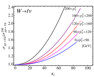
Figure 8: $Vh$ enhancement with $\kappa_{c}$ from the new production mechanism, using the selection cuts ATLAS.

For $c$-tagging II and III, we can only assume the uncorrelated scenario because the assumption for the correlated scenario leads to an inequality,

$$\epsilon_{x}^{\text{($c$-tag)}}\leq\epsilon_{x}^{\text{($b$-tag)}}\ \ \text{for all }x=b,c,l.$$ (31)

$c$-tagging II or III with medium $b$-tagging does not satisfy this inequality. However, the $c$-tagger is expected to be less correlated with $b$-tagging after its possible improvement, so it is reasonable to expect the uncorrelated scenario to be realistic.

We emphasize that the correlation of the two taggers are not an issue for the actual experiments because they have the information for the respective jet. We studied the two different scenarios simply because the information is not available for us to take into account the correlation.

A.2 Non-Standard Model $Vh$ production

For large $\kappa_{c}\sim\!\mathcal{O}(10{\rm-}100)$, new contributions to the $Vh$ final states, shown in Fig. 7, become important and the signal strength is modified not only by the branching ratio but also by the production cross section. The contributions to the $Vh$ production cross section at $\sqrt{s}=14$ TeV as a function of $\kappa_{c}$ are presented in Fig. 8 and are roughly given by

$$\frac{\sigma_{pp\to Vh}}{\sigma^{\rm SM}_{pp\to Vh}}\simeq 1+\left(\frac{\kappa_{c}}{60{\rm-}180}\right)^{2}\$$ (32)

for large $\kappa_{c}$. Here, the Higgs coupling to the $W/Z$ is assumed to be SM like, i.e. $\kappa_{V}=1$. We obtained these results using MadGraph 5.2 Alwall et al. (2011) at the parton level and leading order, applying the ATLAS selection cuts for the LHC $14\,$TeV run The ATLAS Collaboration, ATL-PHYS-PUB-2014-011 .

For 100  TeV $pp$ collider, the effect of the new production mechanism is not important because the sensitivity in $\kappa_{c}$ is $\mathcal{O}(1)$. Therefore, we neglect this effect.

References

- Aad et al. (2012) G. Aad et al. (ATLAS Collaboration), Phys.Lett. B716, 1 (2012), arXiv:1207.7214 [hep-ex] .
- Chatrchyan et al. (2012) S. Chatrchyan et al. (CMS Collaboration), Phys.Lett. B716, 30 (2012), arXiv:1207.7235 [hep-ex] .
- Delaunay et al. (2013) C. Delaunay, C. Grojean, and G. Perez, JHEP 1309, 090 (2013), arXiv:1303.5701 [hep-ph] .
- Delaunay et al. (2014a) C. Delaunay, T. Flacke, J. Gonzalez-Fraile, S. J. Lee, G. Panico, et al., JHEP 1402, 055 (2014a), arXiv:1311.2072 [hep-ph] .
- Blanke et al. (2013) M. Blanke, G. F. Giudice, P. Paradisi, G. Perez, and J. Zupan, JHEP 1306, 022 (2013), arXiv:1302.7232 [hep-ph] .
- Mahbubani et al. (2013) R. Mahbubani, M. Papucci, G. Perez, J. T. Ruderman, and A. Weiler, Phys.Rev.Lett. 110, 151804 (2013), arXiv:1212.3328 [hep-ph] .
- Kagan et al. (2009) A. L. Kagan, G. Perez, T. Volansky, and J. Zupan, Phys.Rev. D80, 076002 (2009), arXiv:0903.1794 [hep-ph] .
- Dery et al. (2013) A. Dery, A. Efrati, G. Hiller, Y. Hochberg, and Y. Nir, JHEP 1308, 006 (2013), arXiv:1304.6727 .
- Giudice and Lebedev (2008) G. F. Giudice and O. Lebedev, Phys.Lett. B665, 79 (2008), arXiv:0804.1753 [hep-ph] .
- Da Rold et al. (2013) L. Da Rold, C. Delaunay, C. Grojean, and G. Perez, JHEP 1302, 149 (2013), arXiv:1208.1499 [hep-ph] .
- Dery et al. (2014) A. Dery, A. Efrati, Y. Nir, Y. Soreq, and V. Susic, Phys.Rev. D90, 115022 (2014), arXiv:1408.1371 [hep-ph] .
- Bishara et al. (2015) F. Bishara, J. Brod, P. Uttayarat, and J. Zupan, (2015), arXiv:1504.04022 [hep-ph] .
- Delaunay et al. (2014b) C. Delaunay, T. Golling, G. Perez, and Y. Soreq, Phys.Rev. D89, 033014 (2014b), arXiv:1310.7029 [hep-ph] .
- The ATLAS Collaboration, ATLAS-CONF-2014-011, ATLAS-COM-CONF-2014- (004) The ATLAS Collaboration, ATLAS-CONF-2014-011, ATLAS-COM-CONF-2014-004, (2014).
- Aad et al. (2014a) G. Aad et al. (ATLAS Collaboration), (2014a), arXiv:1409.6212 [hep-ex] .
- Aad et al. (2015a) G. Aad et al. (ATLAS Collaboration), (2015a), arXiv:1501.04943 [hep-ex] .
- Khachatryan et al. (2014a) V. Khachatryan et al. (CMS Collaboration), JHEP 1409, 087 (2014a), arXiv:1408.1682 [hep-ex] .
- Chatrchyan et al. (2014a) S. Chatrchyan et al. (CMS Collaboration), Phys.Rev. D89, 012003 (2014a), arXiv:1310.3687 [hep-ex] .
- Chatrchyan et al. (2014b) S. Chatrchyan et al. (CMS Collaboration), JHEP 1405, 104 (2014b), arXiv:1401.5041 [hep-ex] .
- Aad et al. (2014b) G. Aad et al. (ATLAS Collaboration), Phys.Lett. B738, 68 (2014b), arXiv:1406.7663 [hep-ex] .
- Khachatryan et al. (2014b) V. Khachatryan et al. (CMS Collaboration), (2014b), arXiv:1410.6679 [hep-ex] .
- Perez et al. (2015) G. Perez, Y. Soreq, E. Stamou, and K. Tobioka, (2015), arXiv:1503.00290 [hep-ph] .
- Bodwin et al. (2013) G. T. Bodwin, F. Petriello, S. Stoynev, and M. Velasco, Phys.Rev. D88, 053003 (2013), arXiv:1306.5770 [hep-ph] .
- Kagan et al. (2014) A. L. Kagan, G. Perez, F. Petriello, Y. Soreq, S. Stoynev, et al., (2014), arXiv:1406.1722 [hep-ph] .
- Isidori et al. (2014) G. Isidori, A. V. Manohar, and M. Trott, Phys.Lett. B728, 131 (2014), arXiv:1305.0663 [hep-ph] .
- Mangano and Melia (2014) M. Mangano and T. Melia, (2014), arXiv:1410.7475 [hep-ph] .
- Huang and Petriello (2014) T.-C. Huang and F. Petriello, (2014), arXiv:1411.5924 [hep-ph] .
- Grossmann et al. (2015) Y. Grossmann, M. König, and M. Neubert, (2015), arXiv:1501.06569 [hep-ph] .
- Aad et al. (2014c) G. Aad et al. (ATLAS Collaboration), Phys.Rev. D90, 052008 (2014c), arXiv:1407.0608 [hep-ex] .
- Aad et al. (2015b) G. Aad et al. (ATLAS Collaboration), (2015b), arXiv:1501.01325 [hep-ex] .
- ATL (2015) Performance and Calibration of the JetFitterCharm Algorithm for c-Jet Identification, Tech. Rep. ATL-PHYS-PUB-2015-001 (CERN, Geneva, 2015).
- Aad et al. (2015c) G. Aad et al. (ATLAS Collaboration), (2015c), arXiv:1501.03276 [hep-ex] .
- Khachatryan et al. (2015) V. Khachatryan et al. (CMS), (2015), arXiv:1507.03031 [hep-ex] .
- Heinemeyer et al. (2013) S. Heinemeyer et al. (LHC Higgs Cross Section Working Group), (2013), 10.5170/CERN-2013-004, arXiv:1307.1347 [hep-ph] .
- (35) The ATLAS Collaboration, ATL-PHYS-PUB-2014-011, “Search for the decay of the Standard Model Higgs boson in associated production with the ATLAS detector,” (2014).
- Capeans et al. (2010) M. Capeans, G. Darbo, K. Einsweiller, M. Elsing, T. Flick, M. Garcia-Sciveres, C. Gemme, H. Pernegger, O. Rohne, and R. Vuillermet, ATLAS Insertable B-Layer Technical Design Report, Tech. Rep. CERN-LHCC-2010-013. ATLAS-TDR-19 (CERN, Geneva, 2010).
- (37) ATLAS Collaboration, “ATLAS B-physics studies at increased LHC luminosity, potential for CP-violation measurement in the decay,” (2013), ATL-PHYS-PUB-2013-010 .
- Chatrchyan et al. (2013) S. Chatrchyan et al. (CMS Collaboration), JINST 8, P04013 (2013), arXiv:1211.4462 [hep-ex] .
- Chetyrkin et al. (2000) K. Chetyrkin, J. H. Kuhn, and M. Steinhauser, Comput.Phys.Commun. 133, 43 (2000), arXiv:hep-ph/0004189 [hep-ph] .
- Olive et al. (2014) K. Olive et al. (Particle Data Group), Chin.Phys. C38, 090001 (2014).
- Cowan et al. (2011) G. Cowan, K. Cranmer, E. Gross, and O. Vitells, Eur.Phys.J. C71, 1554 (2011), arXiv:1007.1727 [physics.data-an] .
- ATL (2014) Projections for measurements of Higgs boson signal strengths and coupling parameters with the ATLAS detector at a HL-LHC, Tech. Rep. ATL-PHYS-PUB-2014-016 (CERN, Geneva, 2014).
- Alwall et al. (2011) J. Alwall, M. Herquet, F. Maltoni, O. Mattelaer, and T. Stelzer, JHEP 1106, 128 (2011), arXiv:1106.0522 [hep-ph] .
- Altheimer et al. (2014) A. Altheimer, A. Arce, L. Asquith, J. Backus Mayes, E. Bergeaas Kuutmann, et al., Eur.Phys.J. C74, 2792 (2014), arXiv:1311.2708 [hep-ex] .
- Backovic et al. (2013) M. Backovic, J. Juknevich, and G. Perez, JHEP 1307, 114 (2013), arXiv:1212.2977 [hep-ph] .
- Almeida et al. (2010) L. G. Almeida, S. J. Lee, G. Perez, G. Sterman, and I. Sung, Phys.Rev. D82, 054034 (2010), arXiv:1006.2035 [hep-ph] .
- Almeida et al. (2012) L. G. Almeida, O. Erdogan, J. Juknevich, S. J. Lee, G. Perez, et al., Phys.Rev. D85, 114046 (2012), arXiv:1112.1957 [hep-ph] .
- Aad et al. (2013) G. Aad et al. (ATLAS), JHEP 1301, 116 (2013), arXiv:1211.2202 [hep-ex] .
- Campbell and Ellis (2010) J. M. Campbell and R. Ellis, Nucl.Phys.Proc.Suppl. 205-206, 10 (2010), arXiv:1007.3492 [hep-ph] .
- Baer et al. (2013) H. Baer, T. Barklow, K. Fujii, Y. Gao, A. Hoang, et al., (2013), arXiv:1306.6352 [hep-ph] .
- Bicer et al. (2014) M. Bicer et al. (TLEP Design Study Working Group), JHEP 1401, 164 (2014), arXiv:1308.6176 [hep-ex] .
- (52) http://indico.cern.ch/event/337673/session/6/contribution/20/material/slides/0.pdf, .
- Bodwin et al. (2014) G. T. Bodwin, H. S. Chung, J.-H. Ee, J. Lee, and F. Petriello, Phys.Rev. D90, 113010 (2014), arXiv:1407.6695 [hep-ph] .
- (54) CMS Collaboration, “Projected Performance of an Upgraded CMS Detector at the LHC and HL-LHC: Contribution to the Snowmass Process,” (2013), arXiv:1307.7135 [hep-ex] .
- ATLAS Collaboration (a) ATLAS Collaboration, “Physics at a High-Luminosity LHC with ATLAS,” (2012a), ATL-PHYS-PUB-2012-004, ATL-COM-PHYS-2012-1455 .
- König and Neubert (2015) M. König and M. Neubert, (2015), arXiv:1505.03870 [hep-ph] .
- Aad et al. (2014d) G. Aad et al. (ATLAS), Phys.Rev. D90, 112015 (2014d), arXiv:1408.7084 [hep-ex] .
- ATLAS Collaboration (b) ATLAS Collaboration, “Expected photon performance in the ATLAS experiment,” (2011b), ATL-PHYS-PUB-2011-007, ATL-COM-PHYS-2010-1051 .
- Sjöstrand et al. (2006) T. Sjöstrand, S. Mrenna, and P. Z. Skands, JHEP 0605, 026 (2006), arXiv:hep-ph/0603175 [hep-ph] .
- Sjöstrand et al. (2015) T. Sjöstrand, S. Ask, J. R. Christiansen, R. Corke, N. Desai, et al., Comput.Phys.Commun. 191, 159 (2015), arXiv:1410.3012 [hep-ph] .