Demonstration of Robust Quantum Gate Tomography via Randomized Benchmarking

Abstract

Typical quantum gate tomography protocols struggle with a self-consistency problem: the gate operation cannot be reconstructed without knowledge of the initial state and final measurement, but such knowledge cannot be obtained without well-characterized gates. A recently proposed technique, known as randomized benchmarking tomography (RBT), sidesteps this self-consistency problem by designing experiments to be insensitive to preparation and measurement imperfections. We implement this proposal in a superconducting qubit system, using a number of experimental improvements including implementing each of the elements of the Clifford group in single ‘atomic’ pulses and custom control hardware to enable large overhead protocols. We show a robust reconstruction of several single-qubit quantum gates, including a unitary outside the Clifford group. We demonstrate that RBT yields physical gate reconstructions that are consistent with fidelities obtained by randomized benchmarking.

I Introduction

All approaches to quantum tomography are forced to make trade-offs given the exponentially increasing resources necessary as the size of the system grows. There has been an aggressive effort from the community to explore alternative approaches that return coarse-grained information in exchange for shorter run times Emerson et al. (2007); da Silva et al. (2011); Moussa et al. (2012). All these techniques rely on some assumptions about the system being characterized. While quantum process tomography (QPT) has been shown to suffer from systematic errors due to incorrect or unverified assumptions about preparation and measurement Merkel et al. (2013), randomized benchmarking (RB) is insensitive to this ignorance and robust against imperfections in the other operations used in the protocol Magesan et al. (2011, 2012a). The trade-off is that randomized benchmarking only provides information about how far away an experiment is from an ideal Clifford group operation, i.e., the average fidelity. In applications where a more complete reconstruction of the operation is necessary, e.g., for debugging purposes, RB fails to provide enough information, while the systematic errors in QPT preclude accurate results.

Randomized benchmarking tomography (RBT) Kimmel et al. (2014) is a recent proposal for near-complete process tomography that inherits the robustness of standard RB and its insensitivity to state preparation and measurement ignorance. Most notably, this technique also allows for the estimation of the average fidelity of any applied gate relative to any unitary operation—in some cases, this estimation can even be done with a polynomial number of experiments.

In this Letter, we apply RBT to reconstruct single-qubit operations in a transmon superconducting qubit, and compare these reconstructions to results obtained via QPT. In particular, we take advantage of the RBT protocol to robustly reconstruct a $\pi/6$ rotation that lies outside the Clifford group. We show that while QPT yields strong non-physical features due to systematic errors, RBT reconstructions remain physical. Moreover, the fidelities estimated by RBT are compatible with fidelities estimated by standard RB.

Unsurprisingly, extracting more information requires more experiments. Like standard QPT and other recent methods for improving upon it Merkel et al. (2013); Blume-Kohout et al. (2013); Stark (2014), RBT comes with an exponential overhead in the total number of experiments. Occasionally, the additional run time leads to drift in parameters of the operation or in state-preparation and measurement errors. This may break a fundamental assumption of most protocols that the parameters are fixed for all rounds of the experiment. Consequently, we describe some strategies for dealing with large experiment-count protocols, including the use of a custom arbitrary waveform generator that operates with very concise sequence descriptions, and readout approaches that improve system stability.

The problem of physically valid reconstructions in tomography is more significant in certain settings. In particular, reconstruction of unitary operations is more sensitive to this issue because such operations are extremal in the set of physically valid operations. Small errors, statistical or otherwise, can easily push estimates outside the physical bounds. To ensure we are near this challenging limit, we endeavor to implement coherence-limited single-qubit unitaries from the Clifford group. A new method we use to achieve this re-introduces $Z$ control to fixed-frequency qubits, creating single-pulse, or atomic, Clifford operations that minimize the average gate time by avoiding multi-pulse decompositions.

II RBT Protocol

We start with a brief description of the RBT protocol. Throughout this discussion, we denote unitary operators in the Clifford group by ${\hat{C}}_{j}$, and the corresponding quantum operation (superoperator) by ${\mathcal{C}}_{j}$. Other operations are denoted by calligraphic fonts as well, e.g., ${\mathcal{E}}$. The sequential composition of two operations ${\mathcal{E}}$ and ${\mathcal{F}}$ is denoted by ${\mathcal{F}}\,{\mathcal{E}}$, meaning ${\mathcal{E}}$ acts first, followed by ${\mathcal{F}}$. This hints at the fact that operations can be represented as matrices and operators as vectors. This representation is known as the Liouville (or Hilbert-Schmidt) representation, and throughout this discussion we will use the Liouville representation in the Pauli basis . Pauli group unitaries are denoted by $X,Y,Z$, while the identity operator is denoted ${{\mathbb{I}}}$.

An operation ${\mathcal{E}}$ is called unital iff ${\mathcal{E}}({{\mathbb{I}}})={{\mathbb{I}}}$. If ${\mathcal{E}}$ is not unital, one can still refer to its unital part, ${\mathcal{E}}^{\prime}$, by ignoring the traceless components of ${\mathcal{E}}({{\mathbb{I}}})$ . This unital part of trace-preserving operations can be decomposed into a linear combination of Clifford group operations Scott (2008); van Dam and Howard (2011); Kimmel et al. (2014). In other words, ${\mathcal{E}}^{\prime}$ can be reconstructed from estimates of overlaps

$$a_{j}=\operatorname{tr}{\mathcal{C}}_{j}^{\dagger}\,{\mathcal{E}},$$ (1)

where ${\mathcal{C}}_{j}$ is a Clifford operation, as long as a sufficiently large linearly independent set of Clifford operations is chosen. For a single-qubit, instead of the full Clifford group we consider

$${\hat{C}}_{1} ={{\mathbb{I}}} {\hat{C}}_{2} ={\mathrm{e}}^{-{\mathrm{i}}{\pi\over 2}X}$$

$${\hat{C}}_{3} ={\mathrm{e}}^{-{\mathrm{i}}{\pi\over 2}Y} {\hat{C}}_{4} ={\mathrm{e}}^{-{\mathrm{i}}{\pi\over 2}Z}$$

$${\hat{C}}_{5} ={\mathrm{e}}^{-{\mathrm{i}}{\pi\over 3}{X+Y+Z\over\sqrt{3}}} {\hat{C}}_{6} ={\mathrm{e}}^{-{\mathrm{i}}{2\pi\over 3}{X+Y+Z\over\sqrt{3}}}$$ (2)

$${\hat{C}}_{7} ={\mathrm{e}}^{-{\mathrm{i}}{\pi\over 3}{X-Y+Z\over\sqrt{3}}} {\hat{C}}_{8} ={\mathrm{e}}^{-{\mathrm{i}}{2\pi\over 3}{X-Y+Z\over\sqrt{3}}}$$

$${\hat{C}}_{9} ={\mathrm{e}}^{-{\mathrm{i}}{\pi\over 3}{X+Y-Z\over\sqrt{3}}} {\hat{C}}_{10} ={\mathrm{e}}^{-{\mathrm{i}}{2\pi\over 3}{X+Y-Z\over\sqrt{3}}}$$

$${\hat{C}}_{11} ={\mathrm{e}}^{-{\mathrm{i}}{\pi\over 3}{-X+Y+Z\over\sqrt{3}}} {\hat{C}}_{12} ={\mathrm{e}}^{-{\mathrm{i}}{2\pi\over 3}{-X+Y+Z\over\sqrt{3}}}.$$

which is a unitary 2-design embedded in the Clifford group Bennett et al. (1996); DiVincenzo et al. (2002); Dankert et al. (2009). We call this group ${{\mathsf{A}}_{4}}$, as it is isomorphic to the alternating group of degree 4, i.e., the group of even permutations of 4 distinct labels. The linear span of the operations in ${{\mathsf{A}}_{4}}$ is 10 dimensional (as is the linear span of the entire Clifford group for single qubits), so in the experiments described here, we take the first 10 of these operations as our linearly independent set. Given an estimate of the overlap vector $\vec{a}=\{a_{1},\ldots,a_{k}\}$, standard unconstrained least-squares inversion yields an estimate of ${\mathcal{E}}^{\prime}$ (See Appendix A).

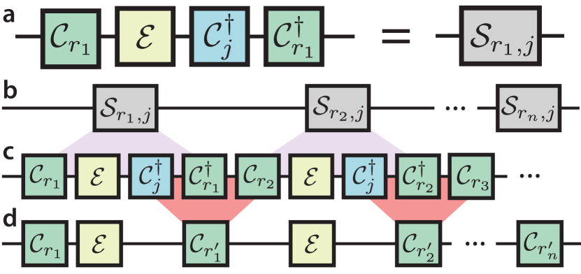
Figure 1: Sequence reduction of an RBT overlap experiment. a The ‘unit cell’, ${\mathcal{S}}_{r,j}$, which is applied iteratively in an RB protocol, b. When written out c, one can identify sections with up to three Clifford operations, e.g. ${\mathcal{C}}_{j}^{\dagger}\,{\mathcal{C}}_{r_{1}}^{\dagger}\,{\mathcal{C}}_{r_{2}}$, which can be compiled into a single gate, ${\mathcal{C}}_{r_{1}^{\prime}}$, also from the Clifford group. The resulting sequence, d, has the same form as a standard IRB experiment, except that we allow ${\mathcal{E}}\not\approx{\mathcal{C}}_{j}$, in which case the action of the complete sequence may not be close to ${{\mathbb{I}}}$.

We estimate the overlaps $a_{j}$ through interleaved RB sequences (IRB) Magesan et al. (2012b); Gaebler et al. (2012), as shown in Fig. 1. That is, we iteratively apply the sequence ${\mathcal{S}}_{r,j}={\mathcal{C}}_{r}^{\dagger}\,{\mathcal{C}}_{j}^{\dagger}\,{\mathcal{E}}\,{\mathcal{C}}_{r}$, where ${\mathcal{C}}_{r}$ is randomly chosen from ${{\mathsf{A}}_{4}}$. We will refer to a sequence ${\mathcal{S}}=\prod_{i}^{n}{\mathcal{S}}_{r_{i},j}$ as a sequence of length $n$, where the $r_{i}$ are chosen independently. In practice, it is convenient to reduce the total sequence length by compiling the compositions of the randomly chosen ${\mathcal{C}}_{r}$’s and the overlap target ${\mathcal{C}}_{j}^{\dagger}$, and applying the corresponding Clifford group operation instead. Choosing the overlap set to be a group ensures that the composed Clifford operations are still in the same set. Consequently, the applied sequences will take the form of alternating random Clifford operations and the target ${\mathcal{E}}$ (see Fig. 1d). As will be discussed later, we exhaustively sample from the set of all sequences of the form of ${\mathcal{S}}$ for a given length, so it is advantageous to sample from a subgroup like ${{\mathsf{A}}_{4}}$ instead of the full Clifford group, in order to limit the total number of experiments.

The expectation of the fidelity between the input and the output of this sequence, averaged over the random choices of Clifford group operations, is Knill et al. (2008); Magesan et al. (2011, 2012a)

$$F_{j,n}=Ap_{j}^{n}+B,$$ (3)

where $p_{j}\in[-\frac{1}{d^{2}-1},1]$ is a decay rate, $d$ is the dimension of the system (here $d=2$), and $A$ and $B$ are factors related to preparation and measurement errors. The decay rate $p_{j}$ is related to the overlap $a_{j}$ by

$$p_{j}=\frac{a_{j}-1}{d^{2}-1},$$ (4)

so that estimates of the decay rates can be used to reconstruct ${\mathcal{E}}$. Equivalently, the $a_{j}$ can be related to the average fidelity between ${\mathcal{E}}$ and ${\mathcal{C}}_{j}$ Horodecki et al. (1999); Nielsen (2002). For small overlaps ($a_{j}<1$), the decay rates are negative, leading to oscillatory decays in the length $n$.

Imperfections in the randomizing operations can be accounted for by characterizing the (ideally) null operation ${\mathcal{E}}_{0}$, a zero-length pulse Magesan et al. (2012b); Kimmel et al. (2014). If only the fidelity of ${\mathcal{E}}_{0}$ to the identity is estimated, the imperfections can only be partially acounted for, leading to very loose bounds on the performance of ${\mathcal{E}}$. However, if the unital part of ${\mathcal{E}}_{0}$ is fully reconstructed, a much more accurate estimate can be made by inversion Kimmel et al. (2014). For any operation ${\mathcal{E}}$ that is reconstructed via RBT, the errors can be accounted for by computing the right and left corrected operations $\widetilde{{\mathcal{E}}}^{\prime}_{R}={\mathcal{E}}^{\prime}\,({\mathcal{E}}_{0}^{\prime})^{-1}$ and $\widetilde{{\mathcal{E}}}^{\prime}_{L}=({\mathcal{E}}_{0}^{\prime})^{-1}\,{\mathcal{E}}^{\prime}$, respectively. The placement of the error operation on the left or right side of ${\mathcal{E}}$ is arbitrary (usually chosen by convention), so either estimate is valid.

A difficulty in experimentally obtaining $p_{j}$ arises from the fact that for most $a_{j}$, the resulting decay $Ap_{j}^{n}$ will rapidly vanish even for small $n$. In fact, if ${\mathcal{E}}$ is close to an ideal Clifford operation, then the $p_{j}$’s in the overlap experiments will be close to $\pm\frac{1}{3}$ or $0$, except when ${\mathcal{C}}_{j}\approx{\mathcal{E}}$. For example, when $n=4$ one needs better than 1% precision in the measured average fidelity to distinguish $(\frac{1}{3})^{4}$ from the mean value of $B$ reliably. One mitigation is to exhaustively sample all random sequences up to a given length. This removes configuration sampling uncertainty from the estimators of $F_{j,n}$ above. The cost of additional experiments may be partially offset by using control hardware with minimal overhead for uploading gate sequences.

III Experimental Implementation

We test the RBT protocol on a single qubit of a 3-transmon, 5-resonator device, described in Ref. Chow et al. (2012). The probed qubit’s coherence times are $T_{1}\approx 5.7\,\mathrm{\mu s}$ and $T_{2}^{\mathrm{echo}}\approx 8.4\,\mathrm{\mu s}$, with anharmonicity $\alpha/2\pi=-221\,\mathrm{MHz}$. The qubit’s readout resonator is coupled to a lumped Josephson parametric amplifier Hatridge et al. (2011) and pumped 17 MHz detuned from the measurement signal to operate it in a phase-preserving mode. The readout assignment fidelity of $\approx 95\%$ is sufficiently high that it is advantageous to convert the measurement outcomes into binary values by thresholding before averaging Ryan et al. (2015). These two choices serve to improve the system stability by reducing sensitivity to the relative phases of the pump and measurement signals, as well as to small voltage fluctuations in the receiver chain.

Qubit control is realized by single sideband modulation of a microwave carrier detuned $\sim 150$MHz from the qubit transition frequency. The shaped modulation signals are generated by a custom arbitrary waveform generator described in Sec. III.2. With the exception of Z rotations which are done with a simple frame-update, we use a fixed-duration pulse of 33.3 ns for all single-qubit gates, and vary the control amplitudes to implement different rotations.

III.1 Atomic Clifford Group Operations

Quantum control in superconducting qubits is usually relaxation limited and so to minimize gate errors it is desirable to keep the gates as short as possible. Typical implementations consider only control about axes in the $XY$ plane or treat $Z$ rotations separately and are forced to decompose rotations about an arbitrary axis into a sequence of rotations—the so-called Euler angle decomposition Nielsen and Chuang (2011). A relevant example of gates that require off-axis rotations are single-qubit Clifford group operations. These can be described as rotations about symmetry axes of the cube in the Bloch sphere, and the cube has symmetries for $\pi$ rotations about the $(1,0,1)$ axis and $2\pi/3$ rotations about the $(1,1,1)$ axis. When implemented with only $XY$ control these can take up to three times longer to implement. Here we show that arbitrary single-qubit gates are possible with a single pulse using conventional control schemes under mild assumptions about the linearity of the control. We term these atomic operations.

In the reference frame rotating at the microwave control frequency, the control Hamiltonian rotates the qubit about a fixed axis in the $XY$-plane. If the qubit is detuned from the microwave drive, then the total Hamiltonian picks up an additional $Z$ component and the effective rotation axis is the vector sum of the drive and detuning terms, giving an arbitrary effective rotation axis. This off-resonance component can be induced by changing the frequency of the qubit or of the microwave drive. Variable frequency qubits struggle to obtain fine-frequency control and introduce non-Markovian effects from the flux bias line. On the other hand, rapidly changing the frequency of a microwave source in a phase coherent manner is a technical challenge. However, experiments already typically provide arbitrary amplitude and phase microwave control with an IQ mixer. This allows us to implement a discrete-time version of a frequency change by linearly ramping the phase of the shaped microwave drive Patt (1992).

The effect of phase ramping on detuning is straightforward to derive from a Trotter expansion of a tilted rotation angle gate. Consider a Hadamard rotation ($\pi$ rotation about the $X+Z$, or $(1,0,1)$ axis). The unitary is given by

$$U_{\text{Had}}=e^{-i\frac{\pi}{2}\frac{1}{\sqrt{2}}\left(X+Z\right)}.$$ (5)

We can then consider a Trotter expansion of the anti-commuting $X$ and $Z$ terms with $\theta=-i\frac{\pi}{2\sqrt{2}}$

$$U_{\text{Had}} =\lim_{n\rightarrow\infty}\left[e^{\frac{\theta}{n}Z}e^{\frac{\theta}{n}X}\right]^{n}$$ (6)

$$=\dots e^{\frac{\theta}{n}Z}e^{\frac{\theta}{n}X}e^{\frac{\theta}{n}Z}e^{\frac{\theta}{n}X}e^{\frac{\theta}{n}Z}e^{\frac{\theta}{n}X}$$

$$=\dots e^{\frac{\theta}{n}Z}e^{\frac{\theta}{n}X}e^{\frac{\theta}{n}Z}\left(e^{\frac{\theta}{n}Z}e^{-\frac{\theta}{n}Z}\right)e^{\frac{\theta}{n}X}e^{\frac{\theta}{n}Z}e^{\frac{\theta}{n}X}$$

$$=\dots e^{\frac{\theta}{n}Z}\left(e^{\frac{2\theta}{n}Z}e^{-\frac{2\theta}{n}Z}\right)e^{\frac{\theta}{n}X}e^{\frac{2\theta}{n}Z}\left[e^{-\frac{\theta}{n}Z}e^{\frac{\theta}{n}X}e^{\frac{\theta}{n}Z}\right]e^{\frac{\theta}{n}X}$$

$$=\dots e^{\frac{3\theta}{n}Z}\left[e^{-\frac{2\theta}{n}Z}e^{\frac{\theta}{n}X}e^{\frac{2\theta}{n}Z}\right]\left[e^{-\frac{\theta}{n}Z}e^{\frac{\theta}{n}X}e^{\frac{\theta}{n}Z}\right]e^{\frac{\theta}{n}X}$$

$$=\lim_{n\rightarrow\infty}e^{\theta Z}\prod_{k=0}^{n-1}\left[e^{-\frac{k\theta}{n}Z}e^{\frac{\theta}{n}X}e^{\frac{k\theta}{n}Z}\right],$$ (7)

where we have injected, in round parenthesis, identity $\pm Z$ rotation blocks. The same approach carries through for shaped pulses with time varying amplitudes. The phase steps dynamically vary with the pulse amplitude to maintain the same effective rotation axis.

Truncating the product in Eq. (7) at finite $n$, corresponding to the number of samples in the control pulse, gives a discrete-time implementation of a frequency shift in terms of XY control (the X components) and per-sample frame updates (the Z components). This is, however, only an approximation (top of Fig. 2). The introduced error is drastically reduced by using a second-order Trotter expansion, or alternatively by defining the phase of each step at the mid-point of the time bin, rather than at the start of the ramp. This second-order version reduces the error to a level which is insignificant compared to other error sources in current implementations.

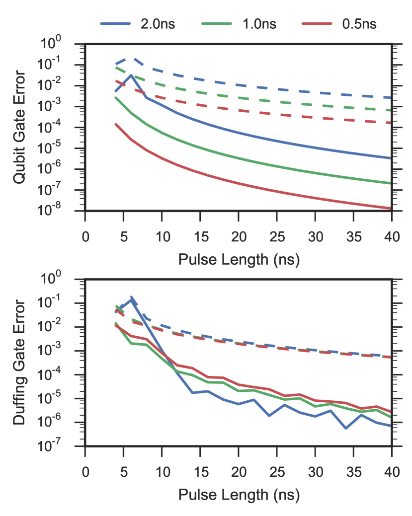
Figure 2: Simulated average gate fidelity Nielsen (2002) for the implementation of a Hadamard gate with a Gaussian pulse shape extending to $\pm 2\sigma$ and varying time steps (colors). (Top) Simulates a qubit model, where the only source of error is discretization error from implementing the frequency shift using phase-ramps. Dashed (solid) lines indicate $1^{\text{st}}$ order ($2^{\text{nd}}$ order) Trotter approximation. (Bottom) Simulates a 5-level Duffing oscillator model of a transmon with $200\,\mathrm{MHz}$ anharmonicity. Dashed lines indicate no DRAG correction whereas solid have $Z$-only DRAG correction. Interplay between the DRAG correction, phase ramping and discretization effects gives non-smooth behavior.

In implementing a detuned pulse we move to a new virtual frame where we acquire phase at a different rate than the qubit’s frame. Thus, when we move back to the qubit frame we must account for the accumulated phase difference. This is represented by the final $Z$ rotation outside the product in Eq. (7). Since we are already working in a rotating frame, this $Z$ rotation may be implemented for free by updating the phase of all subsequent pulses.

When controlling the anharmonic oscillators common to superconducting qubit implementations, additional pulse shaping is necessary to avoid exciting higher energy levels Gambetta et al. (2011). The first-order $Z$-only correction follows through naturally to these phase ramped pulses and their ability to demonstrate high fidelity in a Duffing oscillator model of a transmon is shown in the bottom panel of Fig. 2.

III.2 Custom Control Hardware

Exhaustive sampling of even fairly short RBT overlap experiments (in our case, up to 3 twirling gates) requires implementing thousands of sequences of gates. This poses a practical difficulty for conventional arbitrary waveform generators (AWGs) which require waveforms that are the full duration of each sequence. These AWGs do not take advantage of the relatively small number of primitives that compose RB sequences, i.e., the pulses corresponding to each Clifford operation. Consequently, simply uploading waveform data to a traditional AWG may consume more wall clock time than running the experiment many thousands of times to collect statistics.

To overcome this hurdle, we use a custom arbitrary waveform generator called the Arbitrary Pulse Sequencer (APS). This hardware is programmed using a natural representation for quantum information processing experiments: it uses lists of waveform primitives (pulses as short as 8 samples) and outputs the composite waveform produced by concatenating these primitives without pauses or gaps between successive waveforms. This allows the user to upload only a small set of waveforms, such as a generating set of the Clifford group (e.g. ${{\mathbb{I}}}$, $X$, $Y$, $Z$, $\sqrt{iX}$, $\sqrt{iY}$, $\sqrt{iZ}$), or the ‘atomic’ pulses described above, and re-use these same pulses regardless of the sequence length. This design also has the advantage of dramatically reducing the waveform memory requirements for the APS. In addition, our hardware has the capability to receive new sequence data while simultaneously outputting waveforms. We use dual-port RAM configured as a circular buffer to fill new sequence data behind the sequence read pointer. Consequently, data acquisition can begin with only a small subset of the total sequence loaded onto the APS.

Fast and robust data taking is particularly important to tomography in order to avoid unaccounted for drifts in control or sample parameters, such as fluctuations in the qubit relaxation time. The two improvements described above combine to significantly reduce the overhead of experiments with large numbers of sequences and to reduce sensitivity to drift. For example, using the APS allowed collecting an RBT data set in $\sim 6$ hours. We estimate that with a conventional AWG, the same experiment would take more than twice as long.

IV Results

IV.1 Parameter Estimation Methods

The linear span of single-qubit Clifford group operations is 10 dimensional, and includes all trace-preserving, unital operations. Consequently, an RBT reconstruction requires at least 10 distinct decay experiments, where each observed decay rate $p_{j}$ is related to the trace overlap $a_{j}$ by Eq. (4) . Analytical formulas relating the observed fidelities of each sequence length to the decay rate exist Kimmel et al. (2014), but for the size of the statistical ensemble available to us and the experiment signal-to-noise ratio, this procedure results in large error bars. We remedied this by observing that the fit parameters are not independent across all experiments. In particular, the scaling $A$ and offset $B$ for the decay curves (see Eq. (3)) should be the same across different experiments as long as the characteristics of the state preparation and measurement are stable.

The overlaps with “instantaneous decay” ($p_{j}=0$) suffer from fitting degeneracy between $p_{j}=0$ and poor preparation and measurement ($A=0$). To break the degeneracy, we simultaneously fit a reference slow decay rate ($p_{j}\approx 1$) with each overlap and require the $A$ and $B$ values to be consistent. An appropriate reference comes from a standard RB experiment that estimates the fidelity of the null operation ${\mathcal{E}}_{0}$, which usually has high fidelity to the identity and therefore leads to a slow decay.

Thus, each decay rate $p_{j}$ is found using a four parameter fit of both $F_{j,n}$ and another reference decay, where the parameters are: the reference decay rate (unused in the reconstruction), the decay rate $p_{j}$, a shared scale parameter $A$, and a shared offset parameter $B$, as in Eq. (3). Moreover, because fast decays only lead to a small number of reliable observations, while slow decays lead to many, the figure of merit used in the joint fits is the sum of the mean squared errors of each of the two decays.

The sequence lengths used to estimate each overlap were 1, 2, 3 and $\infty$, where the average fidelities of infinite length sequences were approximated by averaging the single-pulse sequences consisting of the 12 elements of ${{\mathsf{A}}_{4}}$ for the same fixed initial state, which effectively implements a twirl of the initial state. This results in a total of $12+12^{2}+12^{3}+12=1{,}896$ different sequences (length 1 and $\infty$ sequences were repeated 12 times for a total of $2{,}160$ experiments). The resulting decay curves for our implementation of the Hadamard are given in Fig. 3. Since Hadamard $\notin{{\mathsf{A}}_{4}}$, every $p_{j}<1$, and there is no slow decay. In fact, the decay rates $p_{j}\approx\pm\frac{1}{3}$. The curves with $p_{j}<0$ are particularly unusual compared to standard RB experiments due to the oscillatory behavior of the sequence fidelity with length $n$, which occurs for vanishing overlaps $a_{j}\approx 0$.

For each RB, IRB, or RBT sequence we collect 10,000 repetitions, binned into groups of 100. This binning reveals the underlying distribution of the experimental noise, and allows one to resample the data to create bootstrapped confidence intervals. The choice of 100 shots per bin is a trade-off between information about the distribution versus data storage requirements and experiment runtime.

In the analysis here, the fits to the exponential decays were performed by a non-linear least-squares (NLLS) minimization, using Broyden-Fletcher-Goldfarb-Shanno (BFGS) minimization of the joint figure of merit with a starting point obtained from a simple Prony estimate of slow decays de Prony (1795); Peter and Plonka (2013). Confidence intervals were estimated by non-parametric bootstrap percentiles Efron and Tibshirani (1994), using 2000 replications obtained from 100 samples of each of the exhaustive experimental configurations.

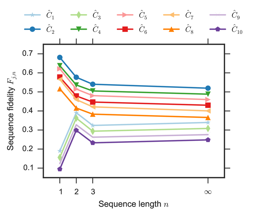
Figure 3: Experimental decay curves from RBT overlap experiments of a Hadamard gate, vertically offset by 0.03 for clarity. “Infinite” length sequences were approximated by averaging outcomes from applying single pulses from ${{\mathsf{A}}_{4}}$. The curves decay rapidly with a rate $|p_{j}|\sim\frac{1}{3}$, and thus the fitting procedure requires more care than standard RB fitting procedures, since only a few points are statistically significant.

IV.2 Reconstruction and fidelities

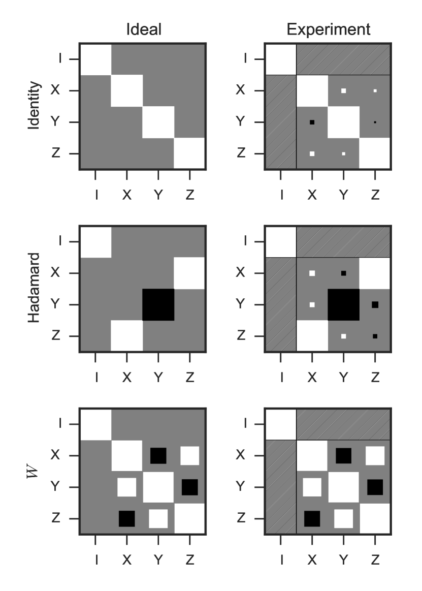
Figure 4: Hinton diagrams Hinton (1986) for the Liouville representations of the ideal operation ${\mathcal{E}}$ (left) and reconstructed unital part of the operation ${\mathcal{E}}^{\prime}$ (right) for the identity operation, Hadamard operation, and ${\hat{W}}={\mathrm{e}}^{-{\mathrm{i}}{\pi\over 12}{X+Y+Z\over\sqrt{3}}}$. The area of each square corresponds to the magnitude of the corresponding matrix element, with the sign represented by white (positive) or black (negative). The hatched areas correspond to parameters not accessible via the RBT protocol.

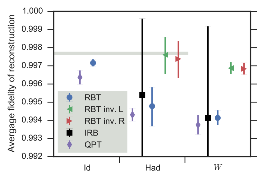
Figure 5: Fidelity estimates for the various reconstructions of the identity, Hadamard, and $W$ gates. The gray bar shows the average fidelity estimate from standard RB for the full single-qubit Clifford group. Error bars indicate 95% confidence intervals for each estimate, except for the IRB points where we show the bounds of the IRB inversion procedure. These bounds are dramatically larger than the uncertainties in the other protocols, extending past the bottom of the figure to roughly 0.985. After removing randomizing error, the RBT fidelity estimate for the Hadamard gate is consistent with standard RB. The lower fidelity of $W$ is potentially due to the gate not being directly calibrated. Coherence-limited control is estimated to produce gate fidelities of 0.9974.

In order to test the protocol, we apply RBT to an implementation of the identity (a zero-length null operation), a Hadamard gate, and the $W$ gate (a $\frac{\pi}{6}$ rotation about the $(1,1,1)$ axis, which is a unitary operation outside the Clifford group). For each tested gate, the fits of the overlap experiments are combined into an overlap vector $\vec{a}=\{a_{1},\ldots,a_{k}\}$. As described in Appendix A, the reconstructed operations ${\mathcal{E}}^{\prime}$ are obtained from least squares inversion. The operations, along with their ideal, noiseless counterparts are depicted in the Pauli-Liouville representation in Fig. 4. In this purely-real representation the unital part excludes most elements of the first row and column. Strictly speaking it also requires the top-left element to be equal to 1 for a trace preserving map, although we have not enforced this constraint in our reconstruction.

We compare RBT reconstructions to standard RB, IRB and QPT. The average fidelities from these approaches for each of the three operations considered are depicted in Fig. 5. The QPT results are adjusted to account for the imperfections in the measurement, under the assumption that these imperfections are independent of the measurement basis (i.e., the data are re-scaled so that the $Z$ measurement spans the range $[-1,1]$). We also compared the RBT reconstruction to a separate IRB estimate of the fidelity of the Hadamard gate, and to a direct estimate of the fidelity of the $W$ gate based on a subset of the decays. Although $W$ is outside the Clifford group, it can be decomposed into a linear combination of Clifford operations. Namely,

$${\mathcal{W}}=\frac{1+\sqrt{3}}{3}{\mathcal{C}}_{1}+\frac{1}{3}{\mathcal{C}}_{5}+\frac{1-\sqrt{3}}{3}{\mathcal{C}}_{6}.$$ (8)

Consequently, one can estimate the fidelity to ${\hat{W}}$ from overlap experiments with just ${\hat{C}}_{1},{\hat{C}}_{5}$, and ${\hat{C}}_{6}$ Kimmel et al. (2014). However, the resulting estimate has the same bounds as the standard IRB protocol, which leads to significantly greater uncertainty in the estimate compared to QPT or RBT. For reference, with our gate durations and sample coherence times, we estimate that coherence-limited control should lead to an average gate fidelity of 0.9974.

Clearly the IRB bounds (black bars) are much looser than the fidelity estimates using the full reconstruction, although all fidelity estimates lie within the IRB bounds, so they are at least consistent. The error bars for the fidelities of the QPT and RBT reconstructions are comparable, and their estimates lie within each other’s error bars (diamond and circle). Importantly, these QPT estimates are non-physical, while the RBT estimates do not suffer from the same problem. However, neither of these estimates are comparable to the fidelity estimate for the identity obtained by RB (gray bar), indicating that the additional error is due to the average error in the randomizing operations, and not just the error in the gate in question.

To fully take advantage of RBT, we use the inverse of the reconstructed null operation ${\mathcal{E}}_{0}^{\prime}$ to remove the error of the randomizing operations from the other reconstructions. As noted earlier in Sec. II, there is freedom to remove this error channel by composing the inverse null operation on the left or right side of the characterized operation, and both may be valid. Consequently, we show both possibilities in the fidelity and negativity estimates. With this error removed, the RBT fidelity estimates (red and green triangles) are much closer to the RB fidelity estimate for the identity. In other words, RBT is able to account for the errors in the randomizing operations without the imprecision that the IRB bounds yield.

IV.3 Systematic errors

Imprecise knowledge about measurement and preparation imperfections is a significant problem in quantum process tomography, because it leads to strong systematic errors in the reconstructions of the quantum process Merkel et al. (2013). While some new techniques aim at performing full reconstruction of all experimental components in a self-consistent manner Dobrovitski et al. (2010); Merkel et al. (2013); Blume-Kohout et al. (2013); Stark (2014), techniques such as RB, RBT, and others aim at getting around this problem by designing experiments that are insensitive to this ignorance Magesan et al. (2011, 2012a, 2012b); Kimmel et al. (2014, 2015).

In order to demonstrate the reduced systematic errors in RBT compared to QPT, we tested the reconstructed process for characteristics such as negative eigenvalues—which, loosely speaking, correspond to negative probabilities, and are therefore non-physical. This technique has been used elsewhere to test for systematic errors in the analysis of tomographic data for quantum states Moroder et al. (2013), but it applies equally well in the quantum process setting, thanks to the Choi-Jamiolkoski isomorphism Jamiołkowski (1972); Choi (1975). This isomorphism makes a one-to-one correspondence between a linear quantum process ${\mathcal{E}}$ and the states $J({\mathcal{E}})$ resulting from applying ${\mathcal{E}}$ to half of a fixed maximally-entangled state. ${\mathcal{E}}$ is considered to be physical if and only if it maps physical states to physical states even when acting on only part of a state—condition known as complete positivity (CP) Jamiołkowski (1972); Choi (1975). This condition is equivalent to requiring that $J({\mathcal{E}})$ be positive (i.e., that it has only positive eigenvalues). While RBT is only able to reconstruct the unital part of ${\mathcal{E}}$, positivity of a single qubit operation is equivalent to positivity of the unital part of that same operation Kimmel et al. (2014), and so these tests can be applied to the reconstructed unital operation ${\mathcal{E}}^{\prime}$.

Following Ref. Moroder et al. (2013), we test ${\mathcal{E}}^{\prime}$ for non-physicality by adaptively estimating the most-negative component of the process and cross-validating it. For each configuration of both RBT and QPT experiments, we divide the measurements into two halves. The first half is used to reconstruct the unital part of the operation, which we denote ${\mathcal{E}}^{\prime}_{1}$. We compute the eigenvector of $J({\mathcal{E}}^{\prime}_{1})$ corresponding to its most negative eigenvalue—this is what we call the negativity witness. The second half is used to obtain an independent estimate of the operation, which we call ${\mathcal{E}}^{\prime}_{2}$, to estimate the expectation value of the negativity witness under $J({\mathcal{E}}^{\prime}_{2})$. Since the parameters of ${\mathcal{E}}^{\prime}_{i}$ are estimated by NLLS instead of projective measurements on $J({\mathcal{E}}^{\prime}_{i})$, we cannot easily use the Hoeffding bounds in Ref. Moroder et al. (2013). Instead, we compute confidence regions using non-parametric bootstrap percentiles, re-sampling only the second half of the samples while holding the negativity witness fixed.

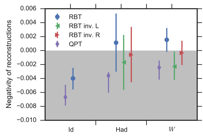
Figure 6: Expectation value of the negativity witness for reconstructed operations using RBT and QPT. The error bars correspond to $95\%$ bootstrapped confidence intervals using 2000 replications of the 50 samples for each experimental configuration used in estimating the expectation value of the entanglement witness.

As Fig. 6 illustrates, the QPT reconstructions have strongly negative eigenvalues even when statistical fluctuations are taken in to account—the $95\%$ confidence intervals are well below zero. With the exception of the identity, all RBT reconstructions are consistent with CP operations—even when the non-physical estimates of the identity are used to separate the error of the randomizing operations from the errors in the gate itself.

The likely culprit for the observed negativity of the RBT estimates is bias in the NLLS estimation of the decay constants. In order to test this, we ran numerical experiments with depolarizing noise leading to fidelities of similar magnitude to what we observed in the experiment, as well as single-shot measurements with probability of error comparable to our experiments. Running our estimation procedure on this artificial data, we also found negativity for the identity reconstruction, with similar negativity to the experiment.

It is possible to obtain physical QPT estimates from unconstrained linear inversion by not compensating for measurement imperfections. This leads to reconstructions without any measurable negativity, at the cost of fidelity estimates that are in the neighborhood of $95\%$. However, this is completely inconsistent with fidelity estimates from RB, so they remain implausible. In other words, QPT estimates that are consistent with RB have statistically significant unphysical properties. By the same token, QPT estimates that are physical are inconsistent with fidelities obtained from RB. RBT estimates, on the other hand, are consistent with physical evolution as well as our best estimates of fidelity for the same gates.

V Summary

We have empirically demonstrated the feasibility of RBT reconstructions of arbitrary single-qubit unitaries. These reconstructions shows significant advantages over standard tomographic reconstruction of quantum operations. Namely, fidelity estimates of the RBT reconstruction are consistent with fidelity estimates obtained through robust methods, while the reconstructed operation is statistically consistent with a physical operation even though such a constraint was not imposed in our reconstruction. We also demonstrated that standard tomographical reconstructions do not satisfy these requirements simultaneously without significant modifications (e.g., using gate-set tomography). However, RBT imposes large costs in terms of experimental runtime and additional analysis complexity. Extending this work to two-qubit process tomography would require either daunting experiment counts for exhaustive sampling, accepting sampling variance in the decay curves, or a modified protocol that yields slow decays that are more ammenable to fitting procedures. Ultimately, however, it remains unclear how to use information obtained from any of the known tomographical protocols for fine-grained debugging of quantum devices. Continued work is necessary to find other robust protocols that answer targeted questions about quantum operations, such as the recent work on robust phase estimation for pulse calibration Kimmel et al. (2015).

Appendix A Least-squares Reconstruction of the unital part ${\mathcal{E}}^{\prime}$

For any given trace preserving quantum operation ${\mathcal{E}}$, the unital part ${\mathcal{E}}^{\prime}$ is linearly related to $\vec{a}$, as described in the main body of the paper, by the equation

$$a_{j}=\operatorname{tr}{\mathcal{C}}_{j}^{\dagger}\,{\mathcal{E}}.$$ (9)

Since the Clifford group operations ${\mathcal{C}}_{j}$ are unital and trace preserving, without loss of generality, this expression can be replaced by

$$a_{j}=\operatorname{tr}{\mathcal{C}}_{j}^{\dagger}\,{\mathcal{E}}^{\prime}.$$ (10)

The explicit reconstruction of ${\mathcal{E}}^{\prime}$ from $\vec{a}$ can be obtained by noting that (10) implies

$$\vec{a}=P\cdot{{\mathrm{vec}({\mathcal{E}}^{\prime})}}$$ (11)

where ${{\mathrm{vec}({\mathcal{E}}^{\prime})}}$ is the vectorization of ${\mathcal{E}}^{\prime}$ and $P$ is the predictor matrix defined as

$$P=\left[\begin{array}[]{c}{{\mathrm{vec}({\hat{C}}_{1}^{*}\otimes{\hat{C}}_{1})}}^{\dagger}\\ {{\mathrm{vec}({\hat{C}}_{2}^{*}\otimes{\hat{C}}_{2})}}^{\dagger}\\ \vdots\end{array}\right].$$ (12)

With these definitions, we have ${\mathcal{E}}^{\prime}=P^{I}\vec{a}$, where $P^{I}$ is the Moore-Penrose pseudo-inverse of $P$ (strict inversion is not possible as $P$ is rank deficient, thanks to Clifford operations spanning only a 10 dimensions space, instead of the 12 dimension space of general trace preserving operations, or the 16 dimensional space of general operations). In the presence of homoscedastic statistical fluctuations, the use of $P^{I}$ corresponds to a least-squares estimate with minimum Euclidean norm, although solving (11) through other equivalent means is preferable to pseudo-inversion, for reasons of numerical stability (the backslash operator in MATLAB and Julia Bezanson et al. (2014), as well as specialized functions in other software packages, provide this functionality).