A Lagrange–Galerkin scheme with a locally linearized velocity for the Navier–Stokes equations

Abstract

We present a Lagrange–Galerkin scheme free from numerical quadrature for the Navier–Stokes equations. Our idea is to use a locally linearized velocity and the backward Euler method in finding the position of fluid particle at the previous time step. Since the scheme can be implemented exactly as it is, the theoretical stability and convergence results are assured. While the conventional Lagrange–Galerkin schemes may encounter the instability caused by numerical quadrature errors, the present scheme is genuinely stable. For the $\mathrm{P}_{2}/\mathrm{P}_{1}$- and $\mathrm{P}_{1}\mathrm{+}/\mathrm{P}_{1}$-finite elements optimal error estimates are proved in $\ell^{\infty}(H^{1})\times\ell^{2}(L^{2})$ norm for the velocity and pressure. We present some numerical results, which reflect these estimates and also show the genuine stability of the scheme.

1 Introduction

The purpose of this paper is to present a Lagrange–Galerkin scheme free from numerical quadrature for the Navier–Stokes equations and to prove the convergence. The Lagrange–Galerkin method, which is also called characteristics finite element method or Galerkin-characteristics method, is a powerful numerical method for flow problems, having such advantages that it is robust for convection-dominated problems and that the resultant matrix to be solved is symmetric. It has, however, a drawback that it may lose the stability when numerical quadrature is employed to integrate composite function terms that characterize the method. Our scheme presented here overcomes this drawback.

Lagrange–Galerkin schemes for the Navier–Stokes equations have been developed in AchdouGuermond2000 ; BermejoSastreSaavedra2012 ; BoukirEtal ; NotsuTabata2009 ; 2015_Notsu-T2 ; Pironneau1982 ; Priestley1994 ; Suli ; see also bibliography therein. After convergence analysis was done successfully by Pironneau Pironneau1982 in a suboptimal rate, the optimal convergence result was obtained by Süli Suli . Optimal convergence results by Lagrange–Galerkin schemes were extended to the multi-step method by Boukir et al. BoukirEtal , to the projection method by Achdou–Guermond AchdouGuermond2000 and to the pressure-stabilized method by Notsu-Tabata 2015_Notsu-T2 . All these results of the stability and convergence are proved under the condition that the integration of the composite function terms is computed exactly. Since it is difficult to perform the exact integration in real problems, numerical quadrature is usually employed. It is, however, reported that instability may occur caused by numerical quadrature error for convection-diffusion problems in MPS ; Priestley1994 ; Tabata2007 ; TSTeng . We observe such instability occurs for the Navier-Stokes equations by numerical examples in this paper.

Several methods have been studied to avoid the instability in BermejoSastreSaavedra2012 ; MPS ; PironneauTabata2010 ; Priestley1994 ; TSTeng . The map of a fluid particle from the present position to the position a time increment $\Delta t$ before (the position is often called foot along the trajectory) is simplified. To find the foot of a particle is nothing but to solve a system of ordinary differential equations (ODEs). Morton et al. MPS solved the ODEs only at the centroids of the elements, and Priestley Priestley1994 did only at the vertices of the elements. The map of the other points is approximated by linear interpolation of those values. It becomes possible to perform the exact integration of the composite function terms with the simplified map. Bermejo et al. BermejoSastreSaavedra2012 used the same simplified map as Priestley1994 to employ a numerical quadrature of high accuracy to the composite function terms for the Navier-Stokes equations. Tanaka et al. TSTeng and Tabata–Uchiumi TabataUchiumi1 approximated the map by a locally linearized velocity and the backward Euler approximation to solve the ODEs for convection-diffusion problems. The approximate map makes possible the exact integration of the composite function terms.

In this paper we prove the convergence of a Lagrange–Galerkin scheme with the same approximate map as TabataUchiumi1 ; TSTeng in the $\mathrm{P}_{2}/\mathrm{P}_{1}$- or $\mathrm{P}_{1}\mathrm{+}/\mathrm{P}_{1}$-element for the Navier–Stokes equations. Since we neither solve the ODEs nor use numerical quadrature, our scheme can be precisely implemented to realize the theoretical results. It is, therefore, a genuinely stable Lagrange–Galerkin scheme. Our convergence results are best possible for the velocity and pressure in $\ell^{\infty}(H^{1})\times\ell^{2}(L^{2})$-norm for both elements as well as for the velocity in $\ell^{\infty}(L^{2})$-norm in the $\mathrm{P}_{1}\mathrm{+}/\mathrm{P}_{1}$-finite element.

The contents of this paper are as follows. In the next section we describe the Navier–Stokes problem and some preparation. In Section 3, after recalling the conventional Lagrange–Galerkin scheme, we present our Lagrange–Galerkin scheme with a locally linearized velocity. In Section 4 we show convergence results, which are proved in Section 5. In Section 6 we show some numerical results, which reflect the theoretical convergence orders and the robustness of the scheme for high Reynolds number problems. In Section 7 we give the conclusions.

2 Preliminaries

We state the problem and prepare the notation used throughout this paper.

Let $\Omega$ be a polygonal or polyhedral domain of $\mathbb{R}^{d}~{}(d=2,3)$ and $T>0$ a time. We use the Sobolev spaces $L^{p}(\Omega)$ with the norm $\left\lVert\cdot\right\rVert_{0,p}$, $W^{s,p}(\Omega)$ and $W^{s,p}_{0}(\Omega)$ with the norm $\left\lVert\cdot\right\rVert_{s,p}$ and the semi-norm $\left\lvert\cdot\right\rvert_{s,p}$ for $p=1,2,\infty$ and a positive integer $s$. When $p=2$, we write $H^{s}(\Omega)=W^{s,2}(\Omega)$ simply and drop the subscript $2$ in the corresponding norms. For the vector-valued function $w\in W^{1,\infty}(\Omega)^{d}$ we define the semi-norm $\lvert w\rvert_{1,\infty}$ by

$$\biggl{\lVert}\biggl{\{}\sum_{i,j=1}^{d}\left(\frac{\partial w_{i}}{\partial x_{j}}\right)^{2}\biggr{\}}^{1/2}\biggr{\rVert}_{0,\infty}.$$

$L^{2}_{0}(\Omega)$ is the subspace of $L^{2}(\Omega)$ with the zero mean. The parenthesis $(\cdot,\cdot)$ shows the $L^{2}(\Omega)^{i}$-inner product for $i=1,d$ or $d\times d$. For $w\in L^{2}(\Omega)^{d}$, $\left\lVert w\right\rVert_{-1}$ stands for the dual norm

$$\sup_{v\in H^{1}_{0}(\Omega)^{d}\setminus\{0\}}\frac{(w,v)}{\left\lVert v\right\rVert_{1}}.$$

For a Sobolev space $X(\Omega)$ we use the abbreviations $H^{m}(X)=H^{m}(0,T;X(\Omega))$ and $C(X)=C([0,T];X(\Omega))$.

$$\begin{split}Z^{m}(t_{1},t_{2})&\equiv\left\{f\in H^{j}(t_{1},t_{2};H^{m-j}(\Omega)^{d});j=0,\dots,m,\left\lVert f\right\rVert_{Z^{m}(t_{1},t_{2})}<\infty\right\},\\ \left\lVert f\right\rVert_{Z^{m}(t_{1},t_{2})}&\equiv\biggl{\{}\sum_{j=0}^{m}\left\lVert f\right\rVert_{H^{j}(t_{1},t_{2};H^{m-j}(\Omega)^{d})}^{2}\biggr{\}}^{1/2}\end{split}$$

and denote $Z^{m}(0,T)$ by $Z^{m}$.

We consider the Navier–Stokes equations: find $(u,p):\Omega\times(0,T)\to\mathbb{R}^{d}\times\mathbb{R}$ such that

$$\begin{split}\frac{Du}{Dt}-\nu\Delta u+\nabla p=f&\quad\text{in~{}}\Omega\times(0,T),\\ \nabla\cdot u=0&\quad\text{in~{}}\Omega\times(0,T),\\ u=0&\quad\text{on~{}}\partial\Omega\times(0,T),\\ u=u^{0}&\quad\text{in~{}}\Omega\text{~{}at~{}}t=0,\end{split}$$ (1)

where $\partial\Omega$ is the boundary of $\Omega$, $\frac{Du}{Dt}\equiv\frac{\partial u}{\partial t}+(u\cdot\nabla)u$ is the material derivative and $\nu>0$ is a viscosity. Functions $f\in C(L^{2})$ and $u^{0}:\Omega\to\mathbb{R}^{d}$ are given.

We define the bilinear forms $a$ on $H^{1}_{0}(\Omega)^{d}\times H^{1}_{0}(\Omega)^{d}$ and $b$ on $H^{1}_{0}(\Omega)^{d}\times L^{2}_{0}(\Omega)$ by

$$a(u,v)\equiv\nu(\nabla u,\nabla v),\quad b(v,q)\equiv-(\nabla\cdot v,q).$$

Then, we can write the weak form of (1) as follows: find $(u,p):(0,T)\to H^{1}_{0}(\Omega)^{d}\times L^{2}_{0}(\Omega)$ such that for $t\in(0,T)$,

$$\left(\frac{Du}{Dt}(t),v\right)+a(u(t),v)+b(v,p(t)) =(f(t),v), \quad\forall v\in H^{1}_{0}(\Omega)^{d},$$ (2a)

$$b(u(t),q) =0, \quad\forall q\in L^{2}_{0}(\Omega),$$ (2b)

with $u(0)=u^{0}$.

Let $u$ be smooth. The characteristic curve $X(t;x,s)$ is defined by the solution of the system of the ordinary differential equations,

$$\frac{dX}{dt}(t;x,s) =u(X(t;x,s),t),\quad t<s,$$ (3a)

$$X(s;x,s) =x.$$ (3b)

Then, we can write the material derivative term $(\frac{\partial}{\partial t}+u\cdot\nabla)u$ as follows:

$$\left(\frac{\partial u}{\partial t}+(u\cdot\nabla)u\right)(X(t),t)=\frac{d}{dt}u(X(t),t).$$

Let $\Delta t>0$ be a time increment. For $w:\Omega\to\mathbb{R}^{d}$ we define the mapping $X_{1}(w):\Omega\to\mathbb{R}^{d}$ by

$$(X_{1}(w))(x)\equiv x-w(x)\Delta t.$$ (4)

Remark 1

The image of $x$ by $X_{1}(u(\cdot,t))$ is nothing but the approximate value of $X(t-\Delta t;x,t)$ obtained by solving (3) by the backward Euler method.

Let $N_{T}\equiv\lfloor T/\Delta t\rfloor$, $t^{n}\equiv n\Delta t$ and $\psi^{n}\equiv\psi(\cdot,t^{n})$ for a function $\psi$ defined in $\Omega\times(0,T)$. For a set of functions $\psi=\left\{\psi^{n}\right\}_{n=0}^{N_{T}}$ and a Sobolev space $X(\Omega)$, two norms $\left\lVert\cdot\right\rVert_{\ell^{\infty}(X)}$ and $\left\lVert\cdot\right\rVert_{\ell^{2}(n_{1},n_{2};X)}$ are defined by

$$\begin{split}\left\lVert\psi\right\rVert_{\ell^{\infty}(X)}&\equiv\max\left\{\left\lVert\psi^{n}\right\rVert_{X(\Omega)};n=0,\dots,N_{T}\right\},\\ \left\lVert\psi\right\rVert_{\ell^{2}(n_{1},n_{2};X)}&\equiv\biggl{(}\Delta t\sum_{n=n_{1}}^{n_{2}}\left\lVert\psi^{n}\right\rVert_{X(\Omega)}^{2}\biggr{)}^{1/2},\end{split}$$

and $\left\lVert\psi\right\rVert_{\ell^{2}(1,N_{T};X)}$ is denoted by $\left\lVert\psi\right\rVert_{\ell^{2}(X)}$. The backward difference operator $\overline{D}_{\Delta t}$ is defined by

$$\overline{D}_{\Delta t}\psi^{n}\equiv\frac{\psi^{n}-\psi^{n-1}}{\Delta t}.$$

Let $\mathcal{T}_{h}$ be a triangulation of $\bar{\Omega}$ and $h\equiv\max_{K\in\mathcal{T}_{h}}\operatorname{diam}(K)$ the maximum element size. Throughout this paper we consider a regular family of triangulations $\{\mathcal{T}_{h}\}_{h\downarrow 0}$. Let $V_{h}\times Q_{h}\subset H_{0}^{1}(\Omega)^{d}\times L_{0}^{2}(\Omega)$ be the $\mathrm{P}_{2}$/$\mathrm{P}_{1}$- or $\mathrm{P}_{1}\mathrm{+}/\mathrm{P}_{1}$-finite element space, which is called Hood-Taylor element or MINI element GiraultRaviart ; MINI . Let

$$\Pi_{h}^{(1)}:C(\bar{\Omega})^{d}\cap H^{1}_{0}(\Omega)^{d}\to V_{h}$$

be the Lagrange interpolation operator to the $\mathrm{P}_{1}$-finite element space. Let $(\widehat{w}_{h},\widehat{r}_{h})\equiv\Pi_{h}^{S}(w,r)\in V_{h}\times Q_{h}$ be the Stokes projection of $(w,r)\in H^{1}_{0}(\Omega)^{d}\times L^{2}_{0}(\Omega)$ defined by

$$a(\widehat{w}_{h},v_{h})+b(v_{h},\widehat{r}_{h}) =a(w,v_{h})+b(v_{h},r),\quad \forall v_{h}\in V_{h},$$ (5a)

$$b(\widehat{w}_{h},q_{h}) =b(w,q_{h}), \forall q_{h}\in Q_{h}.$$ (5b)

We denote by $(\Pi_{h}^{S}(w,r))_{1}$ the first component $\widehat{w}_{h}$ of $\Pi_{h}^{S}(w,r)$.

The symbol $\circ$ stands for the composition of functions, e.g., $(g\circ f)(x)\equiv g(f(x))$.

3 A Lagrange–Galerkin scheme with a locally linearized velocity

The conventional Lagrange–Galerkin scheme, which we call Scheme LG, is described as follows.

Scheme LG

Let $u_{h}^{0}=(\Pi^{S}_{h}(u^{0},0))_{1}$. Find $\left\{(u_{h}^{n},p_{h}^{n})\right\}_{n=1}^{N_{T}}\subset V_{h}\times Q_{h}$ such that

$$\left(\frac{u_{h}^{n}-u_{h}^{n-1}\circ X_{1}(u_{h}^{n-1})}{\Delta t},v_{h}\right)+a(u_{h}^{n},v_{h})+b(v_{h},p_{h}^{n}) =(f^{n},v_{h}),\quad \forall v_{h}\in V_{h},$$

$$b(u_{h}^{n},q_{h}) =0,\quad \forall q_{h}\in Q_{h},$$

for $n=1,\dots,N_{T}$.

Remark 2

Süli Suli used the exact solution $X_{h}^{n-1}$ of the system of ordinary differential equations,

$$\frac{dX_{h}^{n-1}}{dt}(t;x,t^{n}) =u_{h}^{n-1}(X_{h}^{n-1}(t;x,t^{n}),t),\quad t^{n-1}<t<t^{n},$$ (7a)

$$X_{h}^{n-1}(t^{n};x,t^{n}) =x$$ (7b)

instead of $X_{1}(u_{h}^{n-1})$.

By a similar way to Suli combined with BoukirEtal , error estimates

$$\left\lVert u_{h}-u\right\rVert_{\ell^{\infty}(H^{1})},\left\lVert p_{h}-p\right\rVert_{\ell^{2}(L^{2})} \leq c(h^{k}+\Delta t),$$ (8a)

$$\left\lVert u_{h}-u\right\rVert_{\ell^{\infty}(L^{2})} \leq c(h^{k+1}+\Delta t),$$ (8b)

can be proved, where $k=2$ for $\mathrm{P}_{2}/\mathrm{P}_{1}$-element and $k=1$ for $\mathrm{P}_{1}\mathrm{+}/\mathrm{P}_{1}$-element. In the estimate above, the composite function term $(u_{h}^{n-1}\circ X_{1}(u_{h}^{n-1}),v_{h})$ is assumed to be exactly integrated.

Although the function $u_{h}^{n-1}$ is a polynomial on each element $K$, the composite function $u_{h}^{n-1}\circ X_{1}(u_{h}^{n-1})$ is not a polynomial on $K$ in general since the image $X_{1}(u_{h}^{n-1})$ of an element $K$ may spread over plural elements. Hence, it is hard to calculate the composite function term $(u_{h}^{n-1}\circ X_{1}(u_{h}^{n-1}),v_{h})$ exactly. In practice, the following numerical quadrature has been used. Let $g:K\to\mathbb{R}$ be a continuous function. A numerical quadrature $I_{h}[g;K]$ of $\int_{K}g~{}dx$ is defined by

$$I_{h}[g;K]\equiv\operatorname{meas}(K)\sum_{i=1}^{N_{q}}w_{i}g(a_{i}),$$

where $N_{q}$ is the number of quadrature points and $(w_{i},a_{i})\in\mathbb{R}\times K$ is a pair of the weight and the point for $i=1,\dots,N_{q}$. We call the practical scheme using numerical quadrature Scheme LG^′.

Scheme LG^′

Let $u_{h}^{0}=(\Pi^{S}_{h}(u^{0},0))_{1}$. Find $\left\{(u_{h}^{n},p_{h}^{n})\right\}_{n=1}^{N_{T}}\subset V_{h}\times Q_{h}$ such that

$$\frac{1}{\Delta t}(u_{h}^{n},v_{h})-\frac{1}{\Delta t}\sum_{K\in\mathcal{T}_{h}}I_{h}[(u_{h}^{n-1}\circ X_{1}(u_{h}^{n-1}))\cdot v_{h};K]$$

$$+a(u_{h}^{n},v_{h})+b(v_{h},p_{h}^{n}) =(f^{n},v_{h}), \forall v_{h}\in V_{h},$$

$$b(u_{h}^{n},q_{h}) =0, \forall q_{h}\in Q_{h},$$

for $n=1,\dots,N_{T}$.

For convection-diffusion equations it has been reported that numerical quadrature causes the instability MPS ; Priestley1994 ; Tabata2007 ; TabataFujima2006 ; TabataUchiumi1 ; TSTeng . For the Navier-Stokes equations we present numerical results showing the instability of Scheme LG^′ in Section 6.

We now present our Lagrange-Galerkin scheme with a locally linearized velocity. It is free from quadrature and exactly computable. We call it Scheme LG-LLV.

Scheme LG-LLV

Let $u_{h}^{0}=(\Pi^{S}_{h}(u^{0},0))_{1}$. Find $\left\{(u_{h}^{n},p_{h}^{n})\right\}_{n=1}^{N_{T}}\subset V_{h}\times Q_{h}$ such that

$$\!\!\!\!\!\!\biggl{(}\frac{u_{h}^{n}-u_{h}^{n-1}\circ X_{1}(\Pi_{h}^{(1)}u_{h}^{n-1})}{\Delta t},v_{h}\biggr{)}+a(u_{h}^{n},v_{h})+b(v_{h},p_{h}^{n}) =(f^{n},v_{h}), \forall v_{h}\in V_{h},$$ (9a)

$$\!\!\!\!\!\!b(u_{h}^{n},q_{h}) =0, \forall q_{h}\in Q_{h},$$ (9b)

for $n=1\dots,N_{T}$.

In the above scheme the locally linearized velocity $\Pi_{h}^{(1)}u_{h}^{n-1}$ is used in place of the original velocity $u_{h}^{n-1}$. The error caused by the introduction of the approximate velocity $\Pi_{h}^{(1)}u_{h}^{n-1}$ is evaluated properly in Theorems 4.1 and 4.2 in the next section. The following proposition assures that the integration $(u_{h}^{n-1}\circ X_{1}(\Pi_{h}^{(1)}u_{h}^{n-1}),v_{h})$ can be calculated exactly.

Proposition 1

Let $u_{h}$, $v_{h}\in V_{h}$ and $w\in W^{1,\infty}_{0}(\Omega)^{d}$. Suppose $\alpha_{20}\Delta t\lvert w\rvert_{1,\infty}<1$, where $\alpha_{20}$ is the constant defined in (12a) below. Then, $\int_{\Omega}(u_{h}\circ X_{1}(\Pi_{h}^{(1)}w))\cdot v_{h}\ dx$ is exactly computable.

Outline of the proof.  When $u_{h}$ and $v_{h}$ are scalar functions, the result on the exact computability has been proved in TSTeng and (TabataUchiumi1, , Proposition 1). Here, we do not repeat the proof but show only the outline. It is necessary that the inclusion $(X_{1}(\Pi_{h}^{(1)}w))(\Omega)\subset\Omega$ holds to execute the integration of $u_{h}\circ X_{1}(\Pi_{h}^{(1)}w))\cdot v_{h}$ over $\Omega$. The condition $\alpha_{20}\Delta t\lvert w\rvert_{1,\infty}<1$ is sufficient for it by virtue of Lemma 7-(i) and (12a) below. The mapping $X_{1}(\Pi_{h}^{(1)}w)$ is linear on each element. When a mapping $F$ is linear, we have the following general result for any two elements $K_{0}$ and $K_{1}$ and any polynomial $\phi_{h}$ of any order $k$ defined on $K_{1}$. Proposition 1 is proved by applying the following lemma, whose proof is easy, cf. (TabataUchiumi1, , Lemma 1).

Lemma 1

Let $K_{0},K_{1}\in\mathcal{T}_{h}$ and $F:K_{0}\to\mathbb{R}^{d}$ be linear and one-to-one. Let $E_{1}\equiv K_{0}\cap F^{-1}(K_{1})$ and $\operatorname{meas}(E_{1})>0$. Then, the following hold.

1. $E_{1}$ is a polygon ($d=2$) or a polyhedron ($d=3$).

2. $\phi_{h}\circ F_{|E_{1}}\in\mathrm{P}_{k}(E_{1}),\quad\forall\phi_{h}\in\mathrm{P}_{k}(K_{1})$.

Remark 3

In the case of $d=2$, Priestley Priestley1994 approximated $X_{h}^{n-1}(t^{n-1};x,t^{n})$ in (7) by

$$\widetilde{X}_{h}(x)=B_{1}\lambda_{1}(x)+B_{2}\lambda_{2}(x)+B_{3}\lambda_{3}(x),~{}x\in K_{0}$$

on each $K_{0}\in\mathcal{T}_{h}$, where $B_{i}=X_{h}^{n-1}(t^{n-1};A_{i},t^{n})$, $\left\{A_{i}\right\}_{i=1}^{3}$ are vertices of $K_{0}$ and $\left\{\lambda_{i}\right\}_{i=1}^{3}$ are the barycentric coordinates of $K_{0}$ with respect to $\left\{A_{i}\right\}_{i=1}^{3}$. Since $\widetilde{X}_{h}(x)$ is linear in $K_{0}$, the decomposition

$$\int_{K_{0}}(u_{h}^{n-1}\circ\widetilde{X}_{h})\cdot v_{h}\ dx=\sum_{l\in\Lambda(K_{0})}\int_{E_{l}}(u_{h}^{n-1}\circ\widetilde{X}_{h})\cdot v_{h}\ dx,$$

$$\Lambda(K_{0})\equiv\left\{l;K_{0}\cap\widetilde{X}_{h}^{-1}(K_{l})\not=\emptyset\right\},\quad E_{l}\equiv K_{0}\cap\widetilde{X}_{h}^{-1}(K_{l})$$

makes the exact integration possible. However, $B_{i}=X_{h}^{n-1}(t^{n-1};A_{i},t^{n})$ are the solutions of a system of ordinary differential equations and it is not easy to solved it exactly in general since $u_{h}^{n-1}$ is piecewise polynomial. In practice, some numerical method, e.g., Runge–Kutta method, is required, which introduces another error.

4 Main results

We present the main results of error estimates for Scheme LG-LLV, which are proved in the next section. We first state the result when the $\mathrm{P}_{2}/\mathrm{P}_{1}$-element is employed.

Hypothesis 1

The solution of (1) satisfies

$$u\in Z^{2}\cap H^{1}(H^{3}),~{}p\in H^{1}(H^{2}).$$

Remark 4

Hypothesis 1 implies $(u,p)\in C(H^{3}\times H^{2})$, which yields $\nabla\cdot u^{0}=0$.

Hypothesis 2

The sequence $\{\mathcal{T}_{h}\}_{h\downarrow 0}$ satisfies the inverse assumption. In addition, for each $h$, $\forall K\in\mathcal{T}_{h}$ has at least one vertex in $\Omega$.

Theorem 4.1

Let $V_{h}\times Q_{h}$ be the $\mathrm{P}_{2}/\mathrm{P}_{1}$-finite element space. Suppose Hypotheses 1 and 2. Then, there exist positive constants $c_{0}$ and $h_{0}$ such that if $h\in(0,h_{0}]$ and $\Delta t\leq c_{0}h^{d/4}$, the solution $(u_{h},p_{h})\equiv\left\{(u_{h}^{n},p_{h}^{n})\right\}_{n=0}^{N_{T}}$ of Scheme LG-LLV exists and the estimates

$$\left\lVert u_{h}-u\right\rVert_{\ell^{\infty}(H^{1})},\left\lVert p_{h}-p\right\rVert_{\ell^{2}(L^{2})}\leq c_{1}(h^{2}+\Delta t)$$

hold, where $c_{1}$ is a positive constant independent of $h$ and $\Delta t$.

Next, we state the result when the $\mathrm{P}_{1}\mathrm{+}/\mathrm{P}_{1}$-element is employed.

Hypothesis 1^′

The solution of (1) satisfies

$$u\in Z^{2}\cap H^{1}(H^{2}),~{}p\in H^{1}(H^{1}).$$

Remark 5

Hypothesis 1^′ implies $(u,p)\in C(H^{2}\times H^{1})$, which yields $\nabla\cdot u^{0}=0$.

Hypothesis 3

The Stokes problem is regular, that is, for all $g\in L^{2}(\Omega)^{d}$ the solution $(w,r)\in H^{1}_{0}(\Omega)^{d}\times L^{2}_{0}(\Omega)$ of the Stokes problem,

$$\begin{split}-\nu\Delta w+\nabla r=g,&\quad x\in\Omega,\\ \nabla\cdot w=0,&\quad x\in\Omega\end{split}$$

belongs to $H^{2}(\Omega)^{d}\times H^{1}(\Omega)$ and the estimate

$$\lVert(w,r)\rVert_{H^{2}\times H^{1}}\leq c\left\lVert g\right\rVert_{0}.$$

holds, where $c$ is a positive constant independent of $g,w$ and $r$.

Remark 6

Hypothesis 3 holds, for example, if $d=2$ and $\Omega$ is convex GiraultRaviart .

Theorem 4.2

Let $V_{h}\times Q_{h}$ be the $\mathrm{P}_{1}\mathrm{+}/\mathrm{P}_{1}$-finite element space. Suppose Hypotheses 1^′and 2. Then, there exist positive constants $c_{0}$ and $h_{0}$ such that if $h\in(0,h_{0}]$ and $\Delta t\leq c_{0}h^{d/4}$, the solution $(u_{h},p_{h})\equiv\left\{(u_{h}^{n},p_{h}^{n})\right\}_{n=0}^{N_{T}}$ of Scheme LG-LLV exists, and the estimates

$$\left\lVert u_{h}-u\right\rVert_{\ell^{\infty}(H^{1})},\left\lVert p_{h}-p\right\rVert_{\ell^{2}(L^{2})}\leq c_{2}(h+\Delta t)$$ (10)

hold, where $c_{2}$ is a positive constant independent of $h$ and $\Delta t$. Moreover, under Hypothesis 3, the estimate

$$\left\lVert u_{h}-u\right\rVert_{\ell^{\infty}(L^{2})}\leq c_{3}(h^{2}+\Delta t)$$ (11)

holds, where $c_{3}$ is a positive constant independent of $h$ and $\Delta t$.

Remark 7

The convergence proof is easily extended for any pairs satisfying the inf-sup condition. However, the convergence order with respect to the space discretization is bounded by $O(h^{2})$ caused by the locally linearized approximation of the velocity. In fact, in the case of the $\mathrm{P}_{2}/\mathrm{P}_{1}$-element the estimate (8b) with $k=2$ does not hold in Scheme LG-LLV, cf., Example 1 in Section 6.

5 Proofs of the main theorems

We prove Theorem 4.1 in Subsections 5.2–5.4 and Theorem 4.2 in Subsection 5.5.

5.1 Some lemmas

We recall some results used in proving the main theorems. For proofs of Lemmas 2–6 we refer to the cited bibliography.

Lemma 2 (Poincaré’s inequality Ciarlet )

There exists a positive constant $\alpha_{1}(\Omega)$ such that

$$\left\lVert v\right\rVert_{0}\leq\alpha_{1}\left\lvert v\right\rvert_{1},\quad\forall v\in H^{1}_{0}(\Omega)^{d}.$$

Lemma 3 (the Lagrange interpolation Ciarlet )

Suppose $\{\mathcal{T}_{h}\}_{h\downarrow 0}$ is a regular family of triangulations of $\bar{\Omega}$. Let $X_{h}$ be the $\mathrm{P}_{2}$- or $\mathrm{P}_{1}\mathrm{+}$-finite element space and $\Pi_{h}^{(1)}$ be the Lagrange interpolation operator to the $\mathrm{P}_{1}$-finite element space. Then, it holds that

$$\lVert\Pi_{h}^{(1)}v\rVert_{0,\infty}\leq\left\lVert v\right\rVert_{0,\infty},\quad\forall v\in C(\bar{\Omega})^{d},$$

and there exist positive constants $\alpha_{20}\geq 1$, $\alpha_{21}$ and $\alpha_{22}$ such that

$$\lvert\Pi_{h}^{(1)}v\rvert_{1,\infty} \leq\alpha_{20}\left\lvert v\right\rvert_{1,\infty}, \forall v\in W^{1,\infty}(\Omega)^{d},$$ (12a)

$$\lVert\Pi_{h}^{(1)}v-v\rVert_{s} \leq\alpha_{21}h^{2-s}\lvert v\rvert_{2}, s=0,1,~{}\forall v\in H^{2}(\Omega)^{d},$$ (12b)

$$\lVert\Pi_{h}^{(1)}v_{h}\rVert_{0} \leq\alpha_{22}\left\lVert v_{h}\right\rVert_{0}, \forall v_{h}\in X_{h}.$$ (12c)

Remark 8

The inequality (12c) holds since $X_{h}$ is finite-dimensional. If we replace $\Pi_{h}^{(1)}$ by the Clément interpolation operator Clement , this inequality holds for all $v\in L^{2}(\Omega)^{d}$.

Lemma 4 (the inverse inequality Ciarlet ; Suli )

Suppose $\{\mathcal{T}_{h}\}_{h\downarrow 0}$ satisfies the inverse assumption. Let $X_{h}$ be the $\mathrm{P}_{2}$- or $\mathrm{P}_{1}\mathrm{+}$-finite element space. Then, there exist positive constants $\alpha_{30}$ and $\alpha_{31}$ such that

$$\begin{split}\left\lVert v_{h}\right\rVert_{0,\infty}\leq\alpha_{30}h^{-d/6}\left\lVert v_{h}\right\rVert_{1},\quad&\forall v_{h}\in X_{h},\\ \left\lvert v_{h}\right\rvert_{1,\infty}\leq\alpha_{31}h^{-d/2}\left\lvert v_{h}\right\rvert_{1},\quad&\forall v_{h}\in X_{h}.\end{split}$$

Lemma 5 (the inf-sup condition MINI ; BercovierPironneau ; Verfurth1984 )

Suppose Hypothesis 2. Let $V_{h}\times Q_{h}\subset H_{0}^{1}(\Omega)^{d}\times L_{0}^{2}(\Omega)$ be the $\mathrm{P}_{2}/\mathrm{P}_{1}$- or $\mathrm{P}_{1}\mathrm{+}/\mathrm{P}_{1}$-finite element space. Then, there exists a positive constant $\alpha_{4}$ independent of $h$ such that

$$\inf_{q_{h}\in Q_{h}\setminus\left\{0\right\}}\sup_{v_{h}\in V_{h}\setminus\left\{0\right\}}\frac{b(v_{h},q_{h})}{\left\lVert v_{h}\right\rVert_{1}\left\lVert q_{h}\right\rVert_{0}}\geq\alpha_{4}.$$

Lemma 6 (GiraultRaviart )

(i) Suppose Hypothesis 2 and that $V_{h}\times Q_{h}\subset H_{0}^{1}(\Omega)^{d}\times L_{0}^{2}(\Omega)$ is the $\mathrm{P}_{2}/\mathrm{P}_{1}$- or $\mathrm{P}_{1}\mathrm{+}/\mathrm{P}_{1}$-finite element space. Let $(\widehat{w}_{h},\widehat{r}_{h})$ be the Stokes projection of $(w,r)$ defined in (5). Then, there exists a positive constant $\alpha_{50}$ independent of $h$ such that

$$\left\lVert\widehat{w}_{h}-w\right\rVert_{1},\left\lVert\widehat{r}_{h}-r\right\rVert_{0}\leq\alpha_{50}h^{k}\lVert(w,r)\rVert_{H^{k+1}\times H^{k}},$$

where $k=2$ for the $\mathrm{P}_{2}/\mathrm{P}_{1}$-element and $k=1$ for the $\mathrm{P}_{1}\mathrm{+}/\mathrm{P}_{1}$-element.
(ii) Moreover, suppose Hypothesis 3. Then, there exists a positive constant $\alpha_{51}$ such that

$$\left\lVert\widehat{w}_{h}-w\right\rVert_{0}\leq\alpha_{51}h^{k+1}\lVert(w,r)\rVert_{H^{k+1}\times H^{k}},$$

where $k=2$ for the $\mathrm{P}_{2}/\mathrm{P}_{1}$-element and $k=1$ for the $\mathrm{P}_{1}\mathrm{+}/\mathrm{P}_{1}$-element.

Lemma 7

(i) Let $w\in W^{1,\infty}_{0}(\Omega)^{d}$ and $X_{1}(w)$ be the mapping defined in (4). Then, under the condition $\Delta t\lvert w\rvert_{1,\infty}<1$, $X_{1}(w):\Omega\to\Omega$ is bijective.
(ii) Furthermore, under the condition $\Delta t\left\lvert w\right\rvert_{1,\infty}\leq 1/4$, the estimate

$$\frac{1}{2}\leq\det\left(\frac{\partial X_{1}(w)}{\partial x}\right)\leq\frac{3}{2}$$

holds, where $\det(\partial X_{1}(w)/\partial x)$ is the Jacobian.

Proof

The former is proved in (RuiTabata2002, , Proposition 1). We prove the latter only in the case $d=3$ since the proof in $d=2$ is much easier. Let $I$ be the $3\times 3$ identity matrix, $A=(a_{ij})$ and $\boldmath{a}_{j}=(a_{1j},a_{2j},a_{3j})^{T}$, where $a_{ij}=\Delta t\,\partial w_{i}/\partial x_{j}$ for $i,j=1,2,3$. The notation $|\cdot|$ stands for the absolute value, or the Euclidean norm in $\mathbb{R}^{3}$ or $\mathbb{R}^{3\times 3}$. From the condition

$$\left\lvert a\right\rvert=(\left\lvert\boldmath a_{1}\right\rvert^{2}+\left\lvert\boldmath a_{2}\right\rvert^{2}+\left\lvert\boldmath a_{3}\right\rvert^{2})^{1/2}\leq 1/4,$$

we obtain

$$\det(A)\leq\left\lvert\boldmath a_{1}\right\rvert\left\lvert\boldmath a_{2}\right\rvert\left\lvert\boldmath a_{3}\right\rvert\leq\left(\frac{1}{4\sqrt{3}}\right)^{3}.$$

Then, we have

$$\begin{split}&\left\lvert\det\left(\frac{\partial X_{1}(w)}{\partial x}\right)-1\right\rvert=|\det(I-A)-1|\\ =&|-(a_{11}+a_{22}+a_{33})\\ &+a_{11}a_{22}+a_{22}a_{33}+a_{33}a_{11}-a_{12}a_{21}-a_{23}a_{32}-a_{31}a_{13}-\det(A)|\\ \leq&|a_{11}+a_{22}+a_{33}|\\ &+|a_{11}a_{22}+a_{22}a_{33}+a_{33}a_{11}-a_{12}a_{21}-a_{23}a_{32}-a_{31}a_{13}|+|\det(A)|\\ \leq&\sqrt{3}|a|+|a|^{2}+|\det(A)|\leq 1/2,\end{split}$$

which implies the result. ∎

Lemma 8

Let $1\leq q<\infty$, $1\leq p\leq\infty$, $1/p+1/p^{\prime}=1$ and $w_{i}\in W_{0}^{1,\infty}(\Omega)^{d}$, $i=1,2$. Under the condition $\Delta t\lvert w_{i}\rvert_{1,\infty}\leq 1/4$, it holds that, for $\psi\in W^{1,qp^{\prime}}(\Omega)^{d}$,

$$\left\lVert\psi\circ X_{1}(w_{1})-\psi\circ X_{1}(w_{2})\right\rVert_{0,q}\leq 2^{1/(qp^{\prime})}\Delta t\left\lVert w_{1}-w_{2}\right\rVert_{0,pq}\left\lVert\nabla\psi\right\rVert_{0,qp^{\prime}},$$

where $X_{1}(\cdot)$ is defined in (4).

Lemma 8 is a direct consequence of (AchdouGuermond2000, , Lemma 4.5) and Lemma 7-(ii).

Lemma 9

Let $w\in W_{0}^{1,\infty}(\Omega)^{d}$. Under the condition $\Delta t\lvert w\rvert_{1,\infty}\leq 1/4$, there exists a positive constant $\alpha_{6}$ such that, for $\psi\in L^{2}(\Omega)^{d}$,

$$\left\lVert\psi-\psi\circ X_{1}(w)\right\rVert_{-1}\leq\alpha_{6}\Delta t\left\lVert w\right\rVert_{1,\infty}\left\lVert\psi\right\rVert_{0},$$

where $X_{1}(\cdot)$ is defined in (4).

Lemma 9 is obtained from (DouglasRussell1982, , Lemma 1) and Lemma 7-(ii).

5.2 Estimates of $e_{h}^{n}$ under some assumptions

Let

$$(e_{h}^{n},\varepsilon_{h}^{n})\equiv(u_{h}^{n}-\widehat{u}_{h}^{n},p_{h}^{n}-\widehat{p}_{h}^{n}),\quad\eta(t)\equiv u(t)-\widehat{u}_{h}(t),$$ (13)

where $(u,p)$ is the solution of (1), $(\widehat{u}_{h}(t),\widehat{p}_{h}(t))$ is the Stokes projection of $(u(t),p(t))$ defined in (5) and $(u_{h}^{n},p_{h}^{n})$ is the solution of Scheme LG-LLV at the step $n$. From (2), (5) and (9) we have the error equations in $(e_{h}^{n},\varepsilon_{h}^{n})$:

$$\left(\overline{D}_{\Delta t}e_{h}^{n},v_{h}\right)+a(e_{h}^{n},v_{h})+b(v_{h},\varepsilon_{h}^{n}) =\sum_{i=1}^{4}(R_{i}^{n},v_{h}), \forall v_{h}\in V_{h},$$ (14a)

$$b(e_{h}^{n},q_{h}) =0, \forall q_{h}\in Q_{h},$$ (14b)

for $n=1,\dots,N_{T}$, where

$$\begin{split}R_{1}^{n}&\equiv\frac{Du^{n}}{Dt}-\frac{u^{n}-u^{n-1}\circ X_{1}(u^{n-1})}{\Delta t},\\ R_{2}^{n}&\equiv\frac{u^{n-1}\circ X_{1}(\Pi_{h}^{(1)}u_{h}^{n-1})-u^{n-1}\circ X_{1}(u^{n-1})}{\Delta t},\\ R_{3}^{n}&\equiv\frac{\eta^{n}-\eta^{n-1}\circ X_{1}(\Pi_{h}^{(1)}u_{h}^{n-1})}{\Delta t},\quad R_{4}^{n}\equiv-\frac{e_{h}^{n-1}-e_{h}^{n-1}\circ X_{1}(\Pi_{h}^{(1)}u_{h}^{n-1})}{\Delta t}.\end{split}$$ (15)

Lemma 10

Suppose Hypotheses 1 and 2. Under the condition

$${\Delta t\lvert u^{n-1}\rvert_{1,\infty},~{}\Delta t\lvert\Pi_{h}^{(1)}u_{h}^{n-1}\rvert_{1,\infty}\leq 1/4},$$ (16)

it holds that

$$\left\lVert R_{1}^{n}\right\rVert_{0}\leq \beta_{1}\sqrt{\Delta t}\left\lVert u\right\rVert_{Z^{2}(t^{n-1},t^{n})},$$ (17a)

$$\left\lVert R_{2}^{n}\right\rVert_{0}\leq \beta_{2}\left\lVert e_{h}^{n-1}\right\rVert_{0}+\beta_{3}h^{2}(\lVert(u,p)^{n-1}\rVert_{H^{3}\times H^{2}}+\left\lvert u^{n-1}\right\rvert_{2}),$$ (17b)

$$\left\lVert R_{3}^{n}\right\rVert_{0}\leq \beta_{4}\frac{h^{2}}{\sqrt{\Delta t}}\Bigl{(}\lVert(u,p)\rVert_{H^{1}(t^{n-1},t^{n};H^{3}\times H^{2})}$$

$$+\left\lVert u_{h}^{n-1}\right\rVert_{0,\infty}\lVert(u,p)\rVert_{L^{2}(t^{n-1},t^{n};H^{3}\times H^{2})}\Bigr{)},$$ (17c)

$$\left\lVert R_{4}^{n}\right\rVert_{0}\leq \beta_{5}\left\lVert u_{h}^{n-1}\right\rVert_{0,\infty}\left\lvert e_{h}^{n-1}\right\rvert_{1}$$ (17d)

for $n=1,\dots,N_{T}$, where $\beta_{1}=\beta_{1}(\left\lVert u\right\rVert_{C(W^{1,\infty})})$, $\beta_{2}=\beta_{2}(\left\lvert u\right\rvert_{C(W^{1,\infty})},\alpha_{22})$, $\beta_{3}=\beta_{3}(\left\lvert u\right\rvert_{C(W^{1,\infty})},\alpha_{21},\alpha_{22},\alpha_{50})$, $\beta_{4}=\beta_{4}(\alpha_{50})$, $\beta_{5}=\sqrt{2}$ and the notation $\beta_{i}(A)$ means that a positive constant $\beta_{i}$ depends on a set of parameters $A$.

Proof

We prove (17a). We decompose $R_{1}^{n}$ as follows:

$$\begin{split}R_{1}^{n}(x)=&\biggl{\{}\frac{\partial u^{n}}{\partial t}(x)+(u^{n-1}(x)\cdot\nabla)u^{n}(x)-\frac{u^{n}-u^{n-1}\circ X_{1}(u^{n-1})}{\Delta t}(x)\biggr{\}}\\ &+(u^{n}(x)-u^{n-1}(x))\cdot\nabla u^{n}(x)\equiv R_{11}^{n}(x)+R_{12}^{n}(x).\end{split}$$

Setting

$$y(x,s)=x+(s-1)\Delta t~{}u^{n-1}(x),\quad t(s)=t^{n-1}+s\Delta t,$$

we have

$$\frac{u^{n}-u^{n-1}\circ X_{1}(u^{n-1})}{\Delta t}=\frac{1}{\Delta t}\big{[}u(y(\cdot,s),t(s))\big{]}_{s=0}^{1},$$

which implies that

$$R_{11}^{n} =\frac{\partial u^{n}}{\partial t}+(u^{n-1}\cdot\nabla)u^{n}-\int_{0}^{1}\left\{(u^{n-1}(\cdot)\cdot\nabla)u+\frac{\partial u}{\partial t}\right\}(y(\cdot,s),t(s))ds$$

$$=\Delta t\int_{0}^{1}ds\int_{s}^{1}\left\{\left(u^{n-1}(\cdot)\cdot\nabla+\frac{\partial}{\partial t}\right)^{2}u\right\}(y(\cdot,s_{1}),t(s_{1}))ds_{1}$$

$$=\Delta t\int_{0}^{1}s_{1}\left\{\left(u^{n-1}(\cdot)\cdot\nabla+\frac{\partial}{\partial t}\right)^{2}u\right\}(y(\cdot,s_{1}),t(s_{1}))ds_{1}.$$

Hence, we have

$$\|R_{11}^{n}\|_{0} \leq\Delta t\int_{0}^{1}s_{1}\left\|\left\{\left(u^{n-1}(\cdot)\cdot\nabla+\frac{\partial}{\partial t}\right)^{2}u\right\}(y(\cdot,s_{1}),t(s_{1}))\right\|_{0}ds_{1}$$

$$\leq\beta_{1}^{\prime}(\left\lVert u\right\rVert_{C(L^{\infty})})\sqrt{\Delta t}\left\lVert u\right\rVert_{Z^{2}(t^{n-1},t^{n})},$$

where we have used the transformation of independent variables from $x$ to $y$ and $s_{1}$ to $t$ and the estimate $|\det(\partial x/\partial y)|\leq 2$ by virtue of Lemma 7-(ii). It is easy to show

$$\lVert R_{12}^{n}\rVert_{0}\leq\sqrt{\Delta t}\lvert u^{n}\rvert_{1,\infty}\left\lVert\frac{\partial u}{\partial t}\right\rVert_{L^{2}(t^{n-1},t^{n};L^{2})}.$$

From the triangle inequality we get (17a).

We prove (17b). Using Lemma 8 with $q=2$, $p=1$, $p^{\prime}=\infty$, $w_{1}=\Pi_{h}^{(1)}u_{h}^{n-1}$, $w_{2}=u^{n-1}$ and $\psi=u^{n-1}$, we have

$$\begin{split}\lVert R_{2}^{n}\rVert_{0}&\leq\left\lvert u^{n-1}\right\rvert_{1,\infty}\lVert\Pi_{h}^{(1)}u_{h}^{n-1}-u^{n-1}\rVert_{0}\\ &\leq\left\lvert u^{n-1}\right\rvert_{1,\infty}(\lVert\Pi_{h}^{(1)}u_{h}^{n-1}-\Pi_{h}^{(1)}u^{n-1}\rVert_{0}+\lVert\Pi_{h}^{(1)}u^{n-1}-u^{n-1}\rVert_{0}).\end{split}$$

From Lemmas 3 and 6-(i) we evaluate the first term as follows:

$$\begin{split}&\lVert\Pi_{h}^{(1)}u_{h}^{n-1}-\Pi_{h}^{(1)}u^{n-1}\rVert_{0}=\lVert\Pi_{h}^{(1)}(u_{h}^{n-1}-\Pi_{h}^{(1)}u^{n-1})\rVert_{0}\\ \leq&\alpha_{22}\lVert u_{h}^{n-1}-\Pi_{h}^{(1)}u^{n-1}\rVert_{0}\\ \leq&\alpha_{22}(\left\lVert u_{h}^{n-1}-\widehat{u}_{h}^{n-1}\right\rVert_{0}+\left\lVert\widehat{u}_{h}^{n-1}-u^{n-1}\right\rVert_{0}+\lVert u^{n-1}-\Pi_{h}^{(1)}u^{n-1}\rVert_{0})\\ \leq&\alpha_{22}(\lVert e_{h}^{n-1}\rVert_{0}+\alpha_{50}h^{2}\lVert(u,p)^{n-1}\rVert_{H^{3}\times H^{2}}+\alpha_{21}h^{2}\left\lvert u^{n-1}\right\rvert_{2}).\end{split}$$ (18)

The second term is evaluated as follows:

$$\lVert\Pi_{h}^{(1)}u^{n-1}-u^{n-1}\rVert_{0}\leq\alpha_{21}h^{2}\left\lvert u^{n-1}\right\rvert_{2}.$$

Thus, we have

$$\begin{split}\lVert R_{2}^{n}\rVert_{0}\leq\left\lvert u^{n-1}\right\rvert_{1,\infty}&\Bigl{\{}\alpha_{22}(\left\lVert e_{h}^{n-1}\right\rVert_{0}+\alpha_{50}h^{2}\lVert(u,p)^{n-1}\rVert_{H^{3}\times H^{2}})\\ &+\alpha_{21}(1+\alpha_{22})h^{2}\left\lvert u^{n-1}\right\rvert_{2}\Bigr{\}},\end{split}$$

which implies (17b).

We prove (17c). Let

$$y(x)=x+(s-1)\Delta t\Pi_{h}^{(1)}u_{h}^{n-1}(x),\quad t(s)=t^{n-1}+s\Delta t.$$

Since $R_{3}^{n}$ is rewritten as

$$R_{3}^{n}=\int_{0}^{1}\left\{\frac{\partial\eta}{\partial t}+(\Pi_{h}^{(1)}u_{h}^{n-1}(\cdot)\cdot\nabla)\eta\right\}(y(\cdot,s),t(s))ds,$$

we have, by using the change of the variable and Lemma 7-(ii),

$$\left\lVert R_{3}^{n}\right\rVert_{0} \leq\biggl{\lVert}\int_{0}^{1}\left|\frac{\partial\eta}{\partial t}\right|(y(\cdot,s),t(s))ds\biggr{\rVert}_{0}+\biggl{\lVert}\int_{0}^{1}|(\Pi_{h}^{(1)}u_{h}^{n-1}(\cdot)\cdot\nabla)\eta|(y(\cdot,s),t(s))ds\biggr{\rVert}_{0}$$

$$\leq\frac{\sqrt{2}}{\sqrt{\Delta t}}\biggl{(}\left\lVert\frac{\partial\eta}{\partial t}\right\rVert_{L^{2}(t^{n-1},t^{n};L^{2})}+\lVert\Pi_{h}^{(1)}u_{h}^{n-1}\rVert_{0,\infty}\left\lVert\nabla\eta\right\rVert_{L^{2}(t^{n-1},t^{n};L^{2})}\biggr{)}$$

$$\leq\frac{\sqrt{2}\alpha_{50}h^{2}}{\sqrt{\Delta t}}\left(\lVert(u,p)\rVert_{H^{1}(t^{n-1},t^{n};H^{3}\times H^{2})}+\left\lVert u_{h}^{n-1}\right\rVert_{0,\infty}\lVert(u,p)\rVert_{L^{2}(t^{n-1},t^{n};H^{3}\times H^{2})}\right),$$

which implies (17c).

The inequality (17d) is obtained from Lemma 8 with $q=2$, $p=\infty$, $p^{\prime}=1$, $w_{1}=0$, $w_{2}=\Pi_{h}^{(1)}u_{h}^{n-1}$ and $\psi=e_{h}^{n-1}$. ∎

Lemma 11

Suppose Hypotheses 1 and 2. Let $n\in\{1,\cdots,N_{T}\}$ be any integer and let $u_{h}^{n-1}\in V_{h}$ be known. Suppose that $u_{h}^{n-1}$ satisfies

$$b(u_{h}^{n-1},q_{h}) =0, \forall q_{h}\in Q_{h}.$$ (19)

Under the condition (16), there exists a solution $(u_{h}^{n},p_{h}^{n})$ of (9) and it holds that

$$\begin{split}&\left\lVert\overline{D}_{\Delta t}{e_{h}^{n}}\right\rVert_{0}^{2}+\overline{D}_{\Delta t}{(\nu\left\lvert e_{h}^{n}\right\rvert_{1}^{2})}\\ \leq&\beta_{21}(\left\lVert u_{h}^{n-1}\right\rVert_{0,\infty})\nu\left\lvert e_{h}^{n-1}\right\rvert_{1}^{2}+\beta_{22}(\left\lVert u_{h}^{n-1}\right\rVert_{0,\infty})\Bigl{\{}\Delta t\left\lVert u\right\rVert_{Z^{2}(t^{n-1},t^{n})}^{2}\\ &+\frac{h^{4}}{\Delta t}\lVert(u,p)\rVert_{H^{1}(t^{n-1},t^{n};H^{3}\times H^{2})}^{2}+h^{4}\left(\lVert(u,p)^{n-1}\rVert_{H^{3}\times H^{2}}^{2}+\left\lvert u^{n-1}\right\rvert_{2}^{2}\right)\Bigr{\}},\end{split}$$

where $e_{h}^{n}$ is defined in (13), and $\beta_{21}(\xi)$ and $\beta_{22}(\xi)$ are the functions defined in (21) below.

Proof

Since it holds that $\Delta t\lvert\Pi_{h}^{(1)}u_{h}^{n-1}\rvert_{1,\infty}\leq 1/4$, the mapping $X_{1}(\Pi_{h}^{(1)}u_{h}^{n-1}):\Omega\to\Omega$ is bijective from Lemma 7-(i). Hence, there exists a solution $(u_{h}^{n},p_{h}^{n})$ of (9). Substituting $v_{h}=\overline{D}_{\Delta t}{e_{h}^{n}}$ in (14a), we have

$$\left\lVert\overline{D}_{\Delta t}{e_{h}^{n}}\right\rVert_{0}^{2}+\overline{D}_{\Delta t}{\left(\frac{\nu}{2}\left\lVert\nabla e_{h}^{n}\right\rVert_{0}^{2}\right)}+b(\overline{D}_{\Delta t}{e_{h}^{n}},\varepsilon_{h}^{n})\leq\sum_{i=1}^{4}(R_{i}^{n},\overline{D}_{\Delta t}{e_{h}^{n}}).$$ (20)

From (19) and (9) the term $b(\overline{D}_{\Delta t}{e_{h}^{n}},\varepsilon_{h}^{n})$ of the left-hand side vanishes. Using Schwarz’ and Young’s inequalities and Lemma 10, we have

$$\begin{split}&\left\lVert\overline{D}_{\Delta t}{e_{h}^{n}}\right\rVert_{0}^{2}+\overline{D}_{\Delta t}{\left(\frac{\nu}{2}\left\lvert e_{h}^{n}\right\rvert_{1}^{2}\right)}\leq 2\biggl{\{}\beta_{1}^{2}\Delta t\left\lVert u\right\rVert_{Z^{2}(t^{n-1},t^{n})}^{2}\\ &+\left(\beta_{2}\left\lVert e_{h}^{n-1}\right\rVert_{0}+\beta_{3}h^{2}(\lVert(u,p)^{n-1}\rVert_{H^{3}\times H^{2}}+\left\lvert u^{n-1}\right\rvert_{2})\right)^{2}\\ &+\beta_{4}^{2}\frac{h^{4}}{\Delta t}\left(\lVert(u,p)\rVert_{H^{1}(t^{n-1},t^{n};H^{3}\times H^{2})}+\left\lVert u_{h}^{n-1}\right\rVert_{0,\infty}\lVert(u,p)\rVert_{L^{2}(t^{n-1},t^{n};H^{3}\times H^{2})}\right)^{2}\\ &+\beta_{5}^{2}\left\lVert u_{h}^{n-1}\right\rVert_{0,\infty}^{2}\left\lvert e_{h}^{n-1}\right\rvert_{1}^{2}\biggr{\}}+\frac{1}{2}\left\lVert\overline{D}_{\Delta t}e_{h}^{n}\right\rVert_{0}^{2},\end{split}$$

which implies that

$$\begin{split}&\overline{D}_{\Delta t}{(\nu\left\lvert e_{h}^{n}\right\rvert_{1}^{2})}+\left\lVert\overline{D}_{\Delta t}{e_{h}^{n}}\right\rVert_{0}^{2}\\ \leq&\beta_{11}\Bigl{(}\left\lVert e_{h}^{n-1}\right\rVert_{0}^{2}+\left\lVert u_{h}^{n-1}\right\rVert_{0,\infty}^{2}\left\lvert e_{h}^{n-1}\right\rvert_{1}^{2}\Bigr{)}+\beta_{12}\Bigl{\{}\Delta t\left\lVert u\right\rVert_{Z^{2}(t^{n-1},t^{n})}^{2}\\ &+\frac{h^{4}}{\Delta t}(\lVert(u,p)\rVert_{H^{1}(t^{n-1},t^{n};H^{3}\times H^{2})}^{2}+\left\lVert u_{h}^{n-1}\right\rVert_{0,\infty}^{2}\lVert(u,p)\rVert_{L^{2}(t^{n-1},t^{n};H^{3}\times H^{2})}^{2})\\ &+h^{4}\left(\lVert(u,p)^{n-1}\rVert_{H^{3}\times H^{2}}^{2}+\left\lvert u^{n-1}\right\rvert_{2}^{2}\right)\Bigr{\}},\end{split}$$

where $\beta_{11}$ and $\beta_{12}$ are constants depending only on $\beta_{1},\dots,\beta_{5}$. Using Poincaré’s inequality $\lVert e_{h}^{n-1}\rVert_{0}\leq\alpha_{1}\lvert e_{h}^{n-1}\rvert_{1}$ and defining the functions $\beta_{21}$ and $\beta_{22}$ by

$$\beta_{21}(\xi)=\frac{\beta_{11}}{\nu}(\alpha_{1}^{2}+\xi^{2}),~{}\beta_{22}(\xi)=\beta_{12}(1+\xi^{2}),$$ (21)

we have the conclusion. ∎

5.3 Definitions of constants $c_{*}$, $c_{0}$ and $h_{0}$

We first define constants $\beta_{21}^{*}$ and $\beta_{22}^{*}$ by

$$\beta_{21}^{*}\equiv\beta_{21}(\left\lVert u\right\rVert_{C(L^{\infty})}+1),~{}\beta_{22}^{*}\equiv\beta_{22}(\left\lVert u\right\rVert_{C(L^{\infty})}+1).$$

We define two positive constants $c_{*}$ and $c_{0}$ by

$$\begin{split}c_{*}\equiv&\big{\{}\nu^{-1}(1+\alpha_{1}^{2})\exp(\beta_{21}^{*}T)\beta_{22}^{*}\big{\}}^{1/2}\max\Bigl{\{}\left\lVert u\right\rVert_{Z^{2}},\Bigl{(}\lVert(u,p)\rVert_{H^{1}(H^{3}\times H^{2})}^{2}\\ &+T\left(\lVert(u,p)\rVert_{C(H^{3}\times H^{2})}^{2}+\left\lvert u\right\rvert_{C(H^{2})}^{2}\right)+\nu\alpha_{50}^{2}\lvert p^{0}\rvert_{2}^{2}\Bigr{)}^{1/2}\Bigr{\}}\end{split}$$

and

$$c_{0}\equiv\frac{1}{4}\sqrt{\frac{1}{\alpha_{20}\alpha_{31}c_{*}}}.$$ (22)

Let a positive constant $h_{0}$ be small enough to satisfy that

$$\alpha_{30}h_{0}^{1-d/6}\left(c_{*}h_{0}+\alpha_{50}h_{0}\lVert(u,p)\rVert_{C(H^{3}\times H^{2})}+\alpha_{21}\left\lvert u\right\rvert_{C(H^{2})}\right)$$

$$+\alpha_{30}c_{*}c_{0}h_{0}^{d/12} \leq 1,$$ (23a)

$$c_{0}\Bigl{\{}\alpha_{31}h_{0}^{1-d/4}\left(c_{*}h_{0}+\alpha_{50}h_{0}\lVert(u,p)\rVert_{C(H^{3}\times H^{2})}+\alpha_{21}\left\lvert u\right\rvert_{C(H^{2})}\right)$$

$$+\alpha_{20}h_{0}^{d/4}\left\lvert u\right\rvert_{C(W^{1,\infty})}\Bigr{\}} \leq\frac{3}{16\alpha_{20}}.$$ (23b)

which are possible since all the powers of $h_{0}$ are positive.

5.4 Induction

For $n=0,\dots,N_{T}$ we define the property P$(n)$ by

(a)

$\displaystyle\nu\left\lvert e_{h}^{n}\right\rvert_{1}^{2}+\left\lVert\overline{D}_{\Delta t}{e_{h}}\right\rVert_{\ell^{2}(1,n;L^{2})}^{2}\leq\exp(\beta_{21}^{*}n\Delta t)\beta_{22}^{*}\Bigl{\{}\Delta t^{2}\left\lVert u\right\rVert_{Z^{2}(t^{0},t^{n})}^{2}\\ +h^{4}(\lVert(u,p)\rVert_{H^{1}(t^{0},t^{n};H^{3}\times H^{2})}^{2}+\lVert(u,p)\rVert_{\ell^{2}(0,n-1;H^{3}\times H^{2})}^{2}+\left\lvert u\right\rvert_{\ell^{2}(0,n-1;H^{2})}^{2})\\ +\nu\left\lvert e_{h}^{0}\right\rvert_{1}^{2}\Bigr{\}}.$

(b)

$\left\lVert u_{h}^{n}\right\rVert_{0,\infty}\leq\left\lVert u\right\rVert_{C(L^{\infty})}+1$.

(c)

$\Delta t\lvert\Pi_{h}^{(1)}u_{h}^{n}\rvert_{1,\infty}\leq 1/4$.

Proof

We first prove that P($n$) holds for $n=0,\dots,N_{T}$ by induction. When $n=0$, the property P(0)-(a) obviously holds with the equality. The properties P(0)-(b) and (c) are proved in similar ways to and easier than P($n$)-(b) and (c) below, we omit the proofs.

Let $n\in\{1,\cdots,N_{T}\}$ be any integer. Supposing that P($k$), $k=1,\dots,n-1$, holds true, we prove that P($n$) holds. We now apply Lemma 11. The condition (19) is satisfied trivially when $n\geq 2$. When $n=1$, from the choice of $u_{h}^{0}$, (5) and Remark 4 we have

$$b(e_{h}^{0},q_{h})=b(u_{h}^{0},q_{h})-b(\widehat{u}_{h}^{0},q_{h})=0-0=0,\quad\forall q_{h}\in Q_{h}.$$ (24)

We consider the condition (16). The former condition follows from $\Delta t\leq c_{0}h^{d/4}$ and (23b) by the inequality

$$\Delta t\lvert u^{n-1}\rvert_{1,\infty}\leq c_{0}h_{0}^{d/4}\lvert u\rvert_{C(W^{1,\infty})}\leq\frac{3}{16\alpha_{20}}\leq 1/4,$$

and the latter condition $\Delta t\lvert\Pi_{h}^{(1)}u_{h}^{n-1}\rvert_{1,\infty}\leq 1/4$ follows from P($n-1$)-(c). Hence, there exists a solution $(u_{h}^{n},p_{h}^{n})$ at the step $n$.

We begin the proof of P($n$)-(a). By putting

$$x_{n}\equiv \nu\left\lvert e_{h}^{n}\right\rvert_{1}^{2},\quad y_{n}\equiv\left\lVert\overline{D}_{\Delta t}e_{h}^{n}\right\rVert_{0}^{2},$$

$$b_{n}\equiv \Delta t\left\lVert u\right\rVert_{Z^{2}(t^{n-1},t^{n})}^{2}$$

$$+h^{4}\left(\tfrac{1}{\Delta t}\lVert(u,p)\rVert_{H^{1}(t^{n-1},t^{n};H^{3}\times H^{2})}^{2}+\lVert(u,p)^{n-1}\rVert_{H^{3}\times H^{2}}^{2}+\left\lvert u^{n-1}\right\rvert_{2}^{2}\right),$$

P($n$)-(a) is rewritten as

$$x_{n}+\Delta t\sum_{i=1}^{n}y_{i}\leq\exp(\beta_{21}^{*}n\Delta t)\beta_{22}^{*}\biggl{(}x_{0}+\Delta t\sum_{i=1}^{n}b_{i}\biggr{)}.$$ (25)

On the other hand, Lemma 11 implies that

$$x_{n}+\Delta ty_{n}\leq(1+\beta_{21}^{*}\Delta t)x_{n-1}+\beta_{22}^{*}\Delta tb_{n},$$

where we have used the inequalities $\beta_{2i}(\left\lVert u_{h}^{n-1}\right\rVert_{0,\infty})\leq\beta_{2i}^{*}$, $i=1,2$, obtained from P($n-1$)-(b). Using the inequalities $1\leq 1+x\leq\exp(x)$ for $x\geq 0$ and P($n-1$)-(a) rewritten by (25), we have

$$\begin{split}&x_{n}+\Delta t\sum_{i=1}^{n}y_{i}=x_{n}+\Delta ty_{n}+\Delta t\sum_{i=1}^{n-1}y_{i}\\ \leq&(1+\beta_{21}^{*}\Delta t)x_{n-1}+\beta_{22}^{*}\Delta tb_{n}+\Delta t\sum_{i=1}^{n-1}y_{i}\\ \leq&(1+\beta_{21}^{*}\Delta t)\exp(\beta_{21}^{*}(n-1)\Delta t)\beta_{22}^{*}\biggl{(}x_{0}+\Delta t\sum_{i=1}^{n-1}b_{i}\biggr{)}+\beta_{22}^{*}\Delta tb_{n}\\ \leq&\exp(\beta_{21}^{*}n\Delta t)\beta_{22}^{*}\biggl{(}x_{0}+\Delta t\sum_{i=1}^{n}b_{i}\biggr{)},\end{split}$$

which is nothing but P($n$)-(a).

Since $u_{h}^{0}$ is the first component of $\Pi_{h}^{S}(u^{0},0)$, we have

$$e_{h}^{0}=u_{h}^{0}-\widehat{u}_{h}^{0}=(\Pi_{h}^{S}(0,-p^{0}))_{1}=((\Pi_{h}^{S}-I)(0,-p^{0}))_{1},$$

which implies $\left\lvert e_{h}^{0}\right\rvert_{1}\leq\alpha_{50}h^{2}\left\lvert p^{0}\right\rvert_{2}$. From P(0)-(a) and the definition of $c_{*}$, we have

$$\left\lVert e_{h}^{n}\right\rVert_{1}\leq c_{*}(h^{2}+\Delta t).$$ (26)

P($n$)-(b) is proved as follows:

$$\left\lVert u_{h}^{n}\right\rVert_{0,\infty}$$

$$\leq \lVert u_{h}^{n}-\Pi_{h}^{(1)}u^{n}\rVert_{0,\infty}+\lVert\Pi_{h}^{(1)}u^{n}\rVert_{0,\infty}$$

$$\leq \alpha_{30}h^{-d/6}\lVert u_{h}^{n}-\Pi_{h}^{(1)}u^{n}\rVert_{1}+\left\lVert u^{n}\right\rVert_{0,\infty}$$ (by Lemmas 4 and 3)

$$\leq \alpha_{30}h^{-d/6}(\left\lVert u_{h}^{n}-\widehat{u}_{h}^{n}\right\rVert_{1}+\left\lVert\widehat{u}_{h}^{n}-u^{n}\right\rVert_{1}+\lVert u^{n}-\Pi_{h}^{(1)}u^{n}\rVert_{1})+\left\lVert u^{n}\right\rVert_{0,\infty}$$

$$\leq \alpha_{30}h^{-d/6}\left(c_{*}(h^{2}+\Delta t)+\alpha_{50}h^{2}\lVert(u,p)^{n}\rVert_{H^{3}\times H^{2}}+\alpha_{21}h\left\lvert u^{n}\right\rvert_{2}\right)+\left\lVert u^{n}\right\rVert_{0,\infty}$$ (by (26), Lemma 6-(i) and Lemma 3)

$$\leq \alpha_{30}h^{1-d/6}\left(c_{*}h+\alpha_{50}h\lVert(u,p)^{n}\rVert_{H^{3}\times H^{2}}+\alpha_{21}\left\lvert u^{n}\right\rvert_{2}\right)+\alpha_{30}c_{*}c_{0}h^{d/12}+\left\lVert u^{n}\right\rVert_{0,\infty} \Delta t\leq c_{0}h^{d/4}$$ (since )

$$\leq 1+\left\lVert u\right\rVert_{C(L^{\infty})}. h\leq h_{0}$$ (since and by (23a))

We prove P($n$)-(c). We can estimate $\left\lvert u_{h}^{n}\right\rvert_{1,\infty}\Delta t$ as follows:

$$\left\lvert u_{h}^{n}\right\rvert_{1,\infty}\Delta t$$

$$\leq (\lvert u_{h}^{n}-\Pi_{h}^{(1)}u^{n}\rvert_{1,\infty}+\lvert\Pi_{h}^{(1)}u^{n}\rvert_{1,\infty})\Delta t$$

$$\leq \{\alpha_{31}h^{-d/2}(\lvert u_{h}^{n}-\Pi_{h}^{(1)}u^{n}\rvert_{1})+\alpha_{20}\left\lvert u^{n}\right\rvert_{1,\infty}\}\Delta t$$ (by Lemmas 4 and 3)

$$\leq \{\alpha_{31}h^{-d/2}(\left\lvert u_{h}^{n}-\widehat{u}_{h}^{n}\right\rvert_{1}+\left\lvert\widehat{u}_{h}^{n}-u^{n}\right\rvert_{1}+\lvert u^{n}-\Pi_{h}^{(1)}u^{n}\rvert_{1})+\alpha_{20}\left\lvert u^{n}\right\rvert_{1,\infty}\}\Delta t$$

$$\leq \Bigl{\{}\alpha_{31}h^{-d/2}\left(c_{*}(h^{2}+\Delta t)+\alpha_{50}h^{2}\lVert(u,p)^{n}\rVert_{H^{3}\times H^{2}}+\alpha_{21}h\left\lvert u^{n}\right\rvert_{2}\right)$$

$$+\alpha_{20}\left\lvert u^{n}\right\rvert_{1,\infty}\Bigr{\}}\Delta t$$ (by (26), Lemma 6-(i) and Lemma 3)

$$\leq c_{0}\left\{\alpha_{31}h^{1-d/4}\left(c_{*}h+\alpha_{50}h\lVert(u,p)^{n}\rVert_{H^{3}\times H^{2}}+\alpha_{21}\left\lvert u^{n}\right\rvert_{2}\right)+\alpha_{20}h^{d/4}\left\lvert u^{n}\right\rvert_{1,\infty}\right\}$$

$$+\alpha_{31}c_{*}c_{0}^{2} \Delta t\leq c_{0}h^{d/4}$$ (since )

$$\leq \frac{3}{16\alpha_{20}}+\frac{1}{16\alpha_{20}}=\frac{1}{4\alpha_{20}}. h\leq h_{0} c_{0}$$ (since , and by (23b) and the definition of )

From this estimate and the definition of $\alpha_{20}$, we have $\Delta t\lvert\Pi_{h}^{(1)}u_{h}^{n}\rvert_{1,\infty}\leq 1/4$.

Thus, we have proved that P($n$) holds for $n=0,\cdots,N_{T}$.

From P($n$)-(a), $n=0,\dots,N_{T}$, we obtain

$$\left\lVert e_{h}\right\rVert_{\ell^{\infty}(H^{1})},\left\lVert\overline{D}_{\Delta t}e_{h}\right\rVert_{\ell(1,N_{T};L^{2})}\leq c_{*}(h^{2}+\Delta t).$$

Using the triangle inequality $\left\lVert u_{h}-u\right\rVert_{\ell^{\infty}(H^{1})}\leq\left\lVert e_{h}\right\rVert_{\ell^{\infty}(H^{1})}+\left\lVert\eta\right\rVert_{\ell^{\infty}(H^{1})}$, we get

$$\left\lVert u_{h}-u\right\rVert_{\ell^{\infty}(H^{1})}\leq c_{1}(h^{2}+\Delta t).$$

We now prove the estimate on the pressure. We can evaluate $\varepsilon_{h}^{n}$ as follows:

$$\left\lVert\varepsilon_{h}^{n}\right\rVert_{0}\leq \frac{1}{\alpha_{4}}\sup_{v_{h}\in V_{h}}\frac{b(v_{h},\varepsilon_{h}^{n})}{\left\lVert v_{h}\right\rVert_{1}}$$ (by Lemma 5)

$$= \frac{1}{\alpha_{4}}\sup_{v_{h}\in V_{h}}\frac{1}{\left\lVert v_{h}\right\rVert_{1}}\biggl{(}\sum_{i=1}^{4}(R_{i}^{n},v_{h})-(\overline{D}_{\Delta t}e_{h}^{n},v_{h})-a(e_{h}^{n},v_{h})\biggr{)}$$ (by (14a))

$$\leq \frac{1}{\alpha_{4}}\biggl{(}\sum_{i=1}^{4}\left\lVert R_{i}^{n}\right\rVert_{0}+\left\lVert\overline{D}_{\Delta t}e_{h}^{n}\right\rVert_{0}+\nu\left\lvert e_{h}^{n}\right\rvert_{1}\biggr{)}$$

$$\leq c\biggl{(}\left\lVert\overline{D}_{\Delta t}e_{h}^{n}\right\rVert_{0}+\nu\left\lvert e_{h}^{n}\right\rvert_{1}+\lVert e_{h}^{n-1}\rVert_{1}+\sqrt{\Delta t}\left\lVert u\right\rVert_{Z^{2}(t^{n-1},t^{n})}+h^{2}\lVert(u,p)^{n-1}\rVert_{H^{3}\times H^{2}}$$

$$+\frac{h^{2}}{\sqrt{\Delta t}}\lVert(u,p)\rVert_{H^{1}(t^{n-1},t^{n};H^{3}\times H^{2})}+h^{2}\left\lvert u^{n-1}\right\rvert_{2}\biggr{)}, n-1$$ (by Lemma 10 and P()-(b))

which implies that, from (26),

$$\left\lVert\varepsilon_{h}\right\rVert_{\ell^{2}(L^{2})}\leq c(\left\lVert\overline{D}_{\Delta t}e_{h}\right\rVert_{\ell^{2}(L^{2})}+h^{2}+\Delta t)\leq c(h^{2}+\Delta t),$$

where $c$ is a positive constant independent of $h$ and $\Delta t$. Using the triangle inequality

$$\left\lVert p_{h}-p\right\rVert_{\ell^{2}(L^{2})}\leq\left\lVert\varepsilon_{h}\right\rVert_{\ell^{2}(L^{2})}+\left\lVert p-\widehat{p}_{h}\right\rVert_{\ell^{2}(L^{2})},$$

we obtain $\left\lVert p_{h}-p\right\rVert_{\ell^{2}(L^{2})}\leq c_{1}(h^{2}+\Delta t)$. ∎

5.5 Proof of Theorem 4.2

In this subsection we prove the result on the $\mathrm{P}_{1}\mathrm{+}/\mathrm{P}_{1}$-element. At first we replace the estimates of $R_{2}^{n}$ and $R_{3}^{n}$ in Lemma 10.

Lemma 10^′

Suppose Hypotheses 1^′ and 2. Under the condition (16) it holds that

$$\left\lVert R_{2}^{n}\right\rVert_{0} \leq\beta_{2}\left\lVert e_{h}^{n-1}\right\rVert_{0}+\beta_{3}(h\lVert(u,p)^{n-1}\rVert_{H^{2}\times H^{1}}+h^{2}\left\lvert u^{n-1}\right\rvert_{2}),$$

$$\left\lVert R_{3}^{n}\right\rVert_{0} \leq\beta_{4}\frac{h}{\sqrt{\Delta t}}\left(\lVert(u,p)\rVert_{H^{1}(t^{n-1},t^{n};H^{2}\times H^{1})}+\left\lVert u_{h}^{n-1}\right\rVert_{0,\infty}\lVert(u,p)\rVert_{L^{2}(t^{n-1},t^{n};H^{2}\times H^{1})}\right)$$

for $n=1,\dots,N_{T}$.

The proof is similar to Lemma 10 by replacing the order $k=2$ by $k=1$ in Lemma 6-(i).

Proof

We only show the outline of the proof for the existence of $(u_{h},p_{h})$ and the inequality (10) since the proof is similar to that of Theorem 4.1. We replace the definition of $c_{*}$ by

$$\begin{split}c_{*}\equiv&\big{\{}\nu^{-1}(1+\alpha_{1}^{2})\exp(\beta_{21}^{*}T)\beta_{22}^{*}\big{\}}^{1/2}\max\Big{\{}\left\lVert u\right\rVert_{Z^{2}},\Big{(}\lVert(u,p)\rVert_{H^{1}(H^{2}\times H^{1})}^{2}\\ &+T\left(\lVert(u,p)\rVert_{C(H^{2}\times H^{1})}^{2}+\left\lvert u\right\rvert_{C(H^{2})}^{2}\right)+\nu\alpha_{50}^{2}\lvert p^{0}\rvert_{1}^{2}\Big{)}^{1/2}\Big{\}},\end{split}$$

redefine $c_{0}$ by (22) with the new $c_{*}$, and replace the condition (23) on $h_{0}$ by

$$\alpha_{30}h_{0}^{1-d/6}\Bigl{(}c_{*}+\alpha_{50}\lVert(u,p)\rVert_{C(H^{2}\times H^{1})}+\alpha_{21}\left\lvert u\right\rvert_{C(H^{2})}\Bigr{)}+\alpha_{30}c_{*}c_{0}h_{0}^{d/12}\leq 1,$$ (27a)

$$c_{0}\Bigl{\{}\alpha_{31}h_{0}^{1-d/4}\Bigl{(}c_{*}+\alpha_{50}\lVert(u,p)\rVert_{C(H^{2}\times H^{1})}+\alpha_{21}\left\lvert u\right\rvert_{C(H^{2})}\Bigr{)}$$

$$\quad+\alpha_{20}h_{0}^{d/4}\left\lvert u\right\rvert_{C(W^{1,\infty})}\Bigr{\}}\leq\frac{3}{16\alpha_{20}}.$$ (27b)

We also replace P($n$)-(a) by

$$\begin{split}&\nu\left\lvert e_{h}^{n}\right\rvert_{1}^{2}+\left\lVert\overline{D}_{\Delta t}{e_{h}}\right\rVert_{\ell^{2}(1,n;L^{2})}^{2}\leq\exp(\beta_{21}^{*}n\Delta t)\beta_{22}^{*}\Bigl{\{}\Delta t^{2}\left\lVert u\right\rVert_{Z^{2}(t^{0},t^{n})}^{2}\\ &+h^{2}\left(\lVert(u,p)\rVert_{H^{1}(t^{0},t^{n};H^{2}\times H^{1})}^{2}+\lVert(u,p)\rVert_{\ell^{2}(0,n-1;H^{2}\times H^{1})}^{2}+\left\lvert u\right\rvert_{\ell^{2}(0,n-1;H^{2})}^{2}\right)+\nu\left\lvert e_{h}^{0}\right\rvert_{1}^{2}\Bigr{\}}.\end{split}$$

P($n$)-(a) implies the estimate

$$\left\lVert e_{h}^{n}\right\rVert_{1}\leq c_{*}(h+\Delta t).$$ (28)

The choice (27) is sufficient to derive P($n$)-(b) and (c). Hence, the existence of the solution and the estimate (10) are obtained similarly.

We now prove the estimate (11), following Suli except the introduction of $X_{1}(\Pi_{h}^{(1)}u_{h}^{n-1})$. Substituting $(v_{h},q_{h})=(e_{h}^{n},\varepsilon_{h}^{n})$ in (14), we have

$$\frac{1}{2}\overline{D}_{\Delta t}\left\lVert e_{h}^{n}\right\rVert_{0}^{2}+\frac{1}{2\Delta t}\left\lVert e_{h}^{n}-e_{h}^{n-1}\right\rVert_{0}^{2}+\nu\left\lvert e_{h}^{n}\right\rvert_{1}^{2}=\sum_{i=1}^{4}(R_{i}^{n},e_{h}^{n}),$$ (29)

where $R_{i}$, $i=1,\cdots,4$, are defined in (15). The term $(R_{1}^{n},e_{h}^{n})$ is evaluated by (17a). From Lemma 6-(ii) we have

$$\left\lVert\widehat{u}_{h}^{n-1}-u^{n-1}\right\rVert_{0}\leq\alpha_{51}h^{2}\lVert(u,p)^{n-1}\rVert_{H^{2}\times H^{1}}.$$

Using this estimate in the last line in (18), we have

$$(R_{2}^{n},e_{h}^{n})\leq\left\lVert R_{2}^{n}\right\rVert_{0}\left\lVert e_{h}^{n}\right\rVert_{0}\leq\{\beta_{2}\left\lVert e_{h}^{n-1}\right\rVert_{0}+\beta_{3}^{\prime}h^{2}(\lVert(u,p)^{n-1}\rVert_{H^{2}\times H^{1}}+\left\lvert u^{n-1}\right\rvert_{2})\}\left\lVert e_{h}^{n}\right\rVert_{0}.$$

We divide the term $(R_{3}^{n},e_{h}^{n})$ as follows:

$$\begin{split}(R_{3}^{n},e_{h}^{n})=&\frac{1}{\Delta t}(\eta^{n}-\eta^{n-1},e_{h}^{n})+\frac{1}{\Delta t}(\eta^{n-1}-\eta^{n-1}\circ X_{1}(\Pi_{h}^{(1)}u^{n-1}),e_{h}^{n})\\ &+\frac{1}{\Delta t}(\eta^{n-1}\circ X_{1}(\Pi_{h}^{(1)}u^{n-1})-\eta^{n-1}\circ X_{1}(\Pi_{h}^{(1)}u_{h}^{n-1}),e_{h}^{n})\\ &\equiv I_{1}+I_{2}+I_{3}.\end{split}$$

The first term $I_{1}$ is evaluated as

$$I_{1}\leq\frac{1}{\sqrt{\Delta t}}\left\lVert\frac{\partial\eta}{\partial t}\right\rVert_{L^{2}(t^{n-1},t^{n};L^{2})}\left\lVert e_{h}^{n}\right\rVert_{0}\leq\frac{\alpha_{51}h^{2}}{\sqrt{\Delta t}}\lVert(u,p)\rVert_{H^{1}(t^{n-1},t^{n};H^{2}\times H^{1})}\left\lVert e_{h}^{n}\right\rVert_{0}.$$

By Lemma 9 the second term $I_{2}$ is evaluated as

$$\begin{split}I_{2}\leq&\alpha_{6}\alpha_{20}\left\lVert u\right\rVert_{C(W^{1,\infty})}\left\lVert\eta^{n-1}\right\rVert_{0}\left\lVert e_{h}^{n}\right\rVert_{1}\\ \leq&\alpha_{6}\alpha_{20}\left\lVert u\right\rVert_{C(W^{1,\infty})}\alpha_{51}h^{2}\lVert(u,p)^{n-1}\rVert_{H^{2}\times H^{1}}\left\lVert e_{h}^{n}\right\rVert_{1}.\end{split}$$

In order to evaluate $I_{3}$ we prepare the estimate

$$\alpha_{30}h^{-d/6}\left\lvert\eta^{n-1}\right\rvert_{1}\leq\alpha_{30}h^{1-d/6}\alpha_{50}\lVert(u,p)^{n-1}\rVert_{H^{2}\times H^{1}}\leq 1,$$

where we have used Lemma 6-(i) and (27a).

Using Lemma 8 with $q=1$, $p=p^{\prime}=2$, $w_{1}=\Pi_{h}^{(1)}u^{n-1}$, $w_{2}=\Pi_{h}^{(1)}u_{h}^{n-1}$ and $\psi=\eta^{n-1}$, Lemma 4, the above estimate and (18), we can evaluate $I_{3}$ as follows:

$$\begin{split}I_{3}\leq&\frac{1}{\Delta t}\lVert\eta^{n-1}\circ X_{1}(\Pi_{h}^{(1)}u^{n-1})-\eta^{n-1}\circ X_{1}(\Pi_{h}^{(1)}u_{h}^{n-1})\rVert_{0,1}\left\lVert e_{h}^{n}\right\rVert_{0,\infty}\\ \leq&\sqrt{2}\alpha_{30}h^{-d/6}\left\lvert\eta^{n-1}\right\rvert_{1}\lVert\Pi_{h}^{(1)}u^{n-1}-\Pi_{h}^{(1)}u_{h}^{n-1}\rVert_{0}\lVert e_{h}^{n}\rVert_{1}\\ \leq&\sqrt{2}\lVert\Pi_{h}^{(1)}u^{n-1}-\Pi_{h}^{(1)}u_{h}^{n-1}\rVert_{0}\lVert e_{h}^{n}\rVert_{1}\\ \leq&\sqrt{2}\alpha_{22}(\lVert e_{h}^{n-1}\rVert_{0}+\alpha_{51}h^{2}\lVert(u,p)^{n-1}\rVert_{H^{2}\times H^{1}}+\alpha_{21}h^{2}\left\lvert u^{n-1}\right\rvert_{2})\left\lVert e_{h}^{n}\right\rVert_{1}.\end{split}$$

In order to evaluate $(R_{4}^{n},e_{h}^{n})$ we prepare the estimate

$$\alpha_{30}h^{-d/6}\left\lvert e_{h}^{n-1}\right\rvert_{1}\leq\alpha_{30}h^{-d/6}c_{*}(h+\Delta t)\leq\alpha_{30}c_{*}h^{-d/6}(h+c_{0}h^{d/4})\leq 1,$$

where we have used (28) and (27a). Using Lemma 9, the above inequality and a similar estimate to $I_{3}$ in $(R_{3}^{n},e_{h}^{n})$, we can evaluate $(R_{4}^{n},e_{h}^{n})$as follows:

$$\begin{split}(R_{4}^{n},e_{h}^{n})=&-\frac{1}{\Delta t}(e_{h}^{n-1}-e_{h}^{n-1}\circ X_{1}(\Pi_{h}^{(1)}u^{n-1}),e_{h}^{n})\\ &-\frac{1}{\Delta t}(e_{h}^{n-1}\circ X_{1}(\Pi_{h}^{(1)}u^{n-1})-e_{h}^{n-1}\circ X_{1}(\Pi_{h}^{(1)}u_{h}^{n-1}),e_{h}^{n})\\ \leq&\alpha_{6}\alpha_{20}\left\lVert u\right\rVert_{C(W^{1,\infty})}\lVert e_{h}^{n-1}\rVert_{0}\left\lVert e_{h}^{n}\right\rVert_{1}\\ &+\sqrt{2}\alpha_{22}(\lVert e_{h}^{n-1}\rVert_{0}+\alpha_{51}h^{2}\lVert(u,p)^{n-1}\rVert_{H^{2}\times H^{1}}+\alpha_{21}h^{2}\left\lvert u^{n-1}\right\rvert_{2})\left\lVert e_{h}^{n}\right\rVert_{1}.\end{split}$$

Combining (29) with these estimates and using Young’s inequality and Poincaré’s inequality $\left\lVert e_{h}^{n}\right\rVert_{0}\leq\alpha_{1}\left\lvert e_{h}^{n}\right\rvert_{1}$, we have,

$$\begin{split}&\frac{1}{2}\overline{D}_{\Delta t}\left\lVert e_{h}^{n}\right\rVert_{0}^{2}+\nu\left\lvert e_{h}^{n}\right\rvert_{1}^{2}\leq\beta_{31}\Bigl{(}\left\lVert e_{h}^{n-1}\right\rVert_{0}+\sqrt{\Delta t}\left\lVert u\right\rVert_{Z^{2}(t^{n-1},t^{n})}\\ &+\frac{h^{2}}{\sqrt{\Delta t}}\lVert(u,p)\rVert_{H^{1}(t^{n-1},t^{n};H^{2}\times H^{1})}+h^{2}\lVert(u,p)^{n-1}\rVert_{H^{2}\times H^{1}}+h^{2}\left\lvert u^{n-1}\right\rvert_{2}\Bigr{)}\left\lVert e_{h}^{n}\right\rVert_{1}\\ \leq&\nu\left\lvert e_{h}^{n}\right\rvert_{1}^{2}+\beta_{32}\left\lVert e_{h}^{n-1}\right\rVert_{0}^{2}+\beta_{33}\Bigl{\{}\Delta t\left\lVert u\right\rVert_{Z^{2}(t^{n-1},t^{n})}^{2}+\frac{h^{4}}{\Delta t}\lVert(u,p)\rVert_{H^{1}(t^{n-1},t^{n};H^{2}\times H^{1})}\\ &+h^{4}\left(\lVert(u,p)^{n-1}\rVert_{H^{2}\times H^{1}}^{2}+\left\lvert u^{n-1}\right\rvert_{2}^{2}\right)\Bigr{\}},\end{split}$$

where $\beta_{31}$, $\beta_{32}$ and $\beta_{33}$ are positive constants independent of $h$ and $\Delta t$. Applying Gronwall’s inequality, we obtain (11). ∎

6 Numerical results

We show numerical results in $d=2$ for the $\mathrm{P}_{2}/\mathrm{P}_{1}$-element. We compare the conventional Scheme LG^′with the present Scheme LG-LLV. For the triangulation of the domain the FreeFem++ FreeFemCite is used. In Scheme LG^′we employ numerical quadrature of seven-point formula of degree five HMS . The relative error $E_{X}$ is defined by

$$E_{X}(\phi)\equiv\frac{\left\lVert\Pi_{h}\phi-\phi_{h}\right\rVert_{X}}{\left\lVert\Pi_{h}\phi\right\rVert_{X}},$$

for $\phi=u$ in $X=\ell^{\infty}(H_{0}^{1})$ and $\ell^{\infty}(L^{2})$, and for $\phi=p$ in $X=\ell^{2}(L^{2})$.

Example 1

In (1), let $\Omega\equiv(0,1)^{2}$, $T=1$. We consider the two cases, $\nu=10^{-2}$ and $10^{-4}$. The functions $f$ and $u^{0}$ are defined so that the exact solution is

$$\begin{split}u_{1}(x,t)&=\phi(x_{1},x_{2},t),\\ u_{2}(x,t)&=-\phi(x_{2},x_{1},t),\\ p(x,t)&=\sin(\pi(x_{1}+2x_{2})+1+t),\end{split}$$

where $\phi(a,b,t)\equiv-\sin(\pi a)^{2}\sin(\pi b)\{\sin(\pi(a+t))+3\sin(\pi(a+2b+t))\}$.

Let $N$ be the division number of each side of $\Omega$. We set $h\equiv 1/N$. Figure 1 shows the triangulation of $\bar{\Omega}$ for $N=16$. The time increment $\Delta t$ is set to be $\Delta t=h^{2}$ ($N=16,23,32,45$ and $64$) or $\Delta t=h^{3}$ ($N=16,19,23,27$ and $32$) so that we can observe the convergence behavior of order $h^{2}$ or $h^{3}$. The purpose of the choice $\Delta t=O(h^{2})$ or $O(h^{3})$ is to examine the theoretical convergence order, but it is not based on the stability condition, which is much weaker as shown in Theorem 4.1.

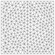
Figure 1: The triangulation of $\bar{\Omega}$ for $N=16$

Table 1: Symbols used in Figs. 2 and 3, and Tables 2 and 3

$\phi$	$u$	$p$	$u$	$u$
$X$	$\ell^{\infty}(H^{1}_{0})$	$\ell^{2}(L^{2})$	$\ell^{\infty}(L^{2})$	$\ell^{\infty}(L^{2})$
$\Delta t$	$h^{2}$	$h^{2}$	$h^{2}$	$h^{3}$
Scheme LG′	$\bullet$	$\blacksquare$	$\blacktriangle$	$\blacktriangledown$
Scheme LG-LLV	$\circ$	$\square$	$\vartriangle$	$\triangledown$

\begin{overpic}[width=113.81102pt]{funcLnu-2forA.pdf} \put(30.0,15.0){\includegraphics[width=25.60747pt]{tri2.pdf}} \end{overpic}

\begin{overpic}[width=113.81102pt]{funcLh3nu-2forA.pdf} \put(30.0,15.0){\includegraphics[width=25.60747pt]{trimid23.pdf}} \end{overpic}

Figure 2: Relative errors $E_{\ell^{\infty}(H^{1}_{0})}(u)$, $E_{\ell^{2}(L^{2})}(p)$, $E_{\ell^{\infty}(L^{2})}(u)$ with $\Delta t=h^{2}$ (left) and $E_{\ell^{\infty}(L^{2})}(u)$ with $\Delta t=h^{3}$ (right) in the case of $\nu=10^{-2}$ in Example 1

Table 2: The values of relative errors and orders in Fig. 2 by Scheme LG^′(top) and Scheme LG-LLV(bottom)

$N$	$\bullet$	order	$\blacksquare$	order	$\blacktriangle$	order
16	8.55e-2		1.63e-1		7.77e-2
23	4.34e-2	1.87	8.40e-2	1.82	4.03e-2	1.81
32	2.30e-2	1.93	4.52e-2	1.88	2.17e-2	1.87
45	1.20e-2	1.90	2.34e-2	1.92	1.13e-2	1.93
64	6.02e-3	1.97	1.18e-2	1.96	5.64e-3	1.96
$N$	$\circ$	order	$\square$	order	$\vartriangle$	order
16	8.97e-2		1.93e-1		7.84e-2
23	4.62e-2	1.83	1.03e-1	1.73	4.10e-2	1.78
32	2.46e-2	1.92	5.44e-2	1.92	2.25e-2	1.82
45	1.29e-2	1.90	2.84e-2	1.91	1.17e-2	1.93
64	6.39e-3	1.99	1.41e-2	1.97	5.81e-3	1.98

$N$	$\blacktriangledown$	order
16	6.45e-3
19	3.73e-3	3.19
23	2.10e-3	3.02
27	1.29e-3	3.02
32	7.57e-4	3.15
$N$	$\triangledown$	order
16	1.48e-2
19	9.19e-3	2.78
23	6.04e-3	2.19
27	3.83e-3	2.85
32	2.72e-3	2.01

\begin{overpic}[width=113.81102pt]{funcLnu-4forA.pdf} \put(27.0,15.0){\includegraphics[width=25.60747pt]{tri2.pdf}} \end{overpic}

\begin{overpic}[width=113.81102pt]{funcLh3nu-4forA.pdf} \put(27.0,15.0){\includegraphics[width=25.60747pt]{trimid23.pdf}} \end{overpic}

Figure 3: Relative errors $E_{\ell^{\infty}(H^{1}_{0})}(u)$, $E_{\ell^{2}(L^{2})}(p)$, $E_{\ell^{\infty}(L^{2})}(u)$ with $\Delta t=h^{2}$ (left) and $E_{\ell^{\infty}(L^{2})}(u)$ with $\Delta t=h^{3}$ (right) in the case of $\nu=10^{-4}$ in Example 1

Table 3: The values of errors and orders of the graphs in Fig. 3 with $\Delta t=h^{2}$ (top) and $\Delta t=h^{3}$ (bottom)

$N$	$\bullet$	order	$\blacksquare$	order	$\blacktriangle$	order
16	1.91e+0		2.14e-1		1.93e-1
23	1.34e+0	0.97	8.97e-2	2.39	8.81e-2	2.16
32	9.42e+0	-5.90	3.48e-1	-4.11	5.28e-1	-5.43
45	4.10e+1	-4.31	1.28e+0	-3.81	1.46e+0	-2.98
64	8.82e+1	-2.18	2.77e+0	-2.20	2.02e+0	-0.93
$N$	$\circ$	order	$\square$	order	$\vartriangle$	order
16	6.72e-1		2.65e-1		2.09e-1
23	3.91e-1	1.50	1.36e-1	1.83	9.88e-2	2.07
32	1.85e-1	2.26	6.98e-2	2.02	4.18e-2	2.60
45	1.27e-1	1.10	3.73e-2	1.84	2.12e-2	1.99
64	7.21e-2	1.61	1.83e-2	2.03	9.78e-3	2.20

$N$	$\blacktriangledown$	order
16	1.55e-1
19	6.64e-2	4.92
23	3.65e-2	3.14
27	1.92e-2	4.01
32	1.02e-2	3.71
$N$	$\triangledown$	order
16	2.47e-1
19	1.05e-1	4.96
23	8.80e-2	0.94
27	6.18e-2	2.20
32	2.97e-2	3.29

Table 1 shows the symbols used in the graphs and tables. Since every graph of the relative error $E_{X}$ versus $h$ is depicted in the logarithmic scale, the slope corresponds to the convergence order. Figure 2 shows the graphs of $E_{\ell^{\infty}(H^{1}_{0})}(u)$, $E_{\ell^{2}(L^{2})}(p)$ and $E_{\ell^{\infty}(L^{2})}(u)$ versus $h$ in the case of $\nu=10^{-2}$. Their values and convergence orders are listed in Table 2. When $\Delta t=h^{2}$, the convergence orders of $E_{\ell^{\infty}(H^{1}_{0})}(u)$ ($\bullet$, $\circ$), $E_{\ell^{2}(L^{2})}(p)$ ($\blacksquare$, $\square$) and $E_{\ell^{\infty}(L^{2})}(u)$ ($\blacktriangle$, $\vartriangle$) are almost 2 in both schemes. When $\Delta t=h^{3}$, the order of $E_{\ell^{\infty}(L^{2})}(u)$ is almost 3 in Scheme LG^′ ($\blacktriangledown$) and 2 in Scheme LG-LLV ($\triangledown$). They reflect the theoretical results.

We consider a higher Reynolds number case. Figure 3 shows the graphs in the case of $\nu=10^{-4}$ and their values are listed in Table 3. When $\Delta t=h^{2}$, all errors increase abnormally at $N=32,45$ and $64$ in Scheme LG^′ ($\bullet$, $\blacksquare$, $\blacktriangle$) while the convergence is observed in Scheme LG-LLV ($\circ$, $\square$, $\vartriangle$) but the order of $E_{\ell^{\infty}(H^{1}_{0})}(u)$ ($\circ$) is less than 2. In order to obtain the theoretical convergence order $O(h^{2})$ in Scheme LG-LLV, it seems that finer meshes will be necessary. When $\Delta t=h^{3}$, the order of $E_{\ell^{\infty}(L^{2})}(u)$ is more than 3 in Scheme LG^′ ($\blacktriangledown$) while it is less than 3 between $N=19$ and $23$, and $N=23$ and $27$ in Scheme LG-LLV ($\triangledown$).

Figure 4: The domain $\Omega$ and the boundary condition (left) and the triangulation of $\Omega$ (right) in Example 2

.

We now consider a cavity problem to see that Scheme LG-LLV is robust for high Reynolds number while Scheme LG^′ is not. This problem is not a homogeneous Dirichlet boundary problem, but it is often used as a benchmark problem. In order to assure the existence of the solution we deal with a regularized cavity problem, where the prescribed velocity is continuous on the boundary.

Example 2

Let $\Omega\equiv(0,1)^{2}$, $f=0$, $u^{0}=0$. We consider the two cases, $\nu=10^{-4}$ and $10^{-5}$. The boundary condition is described in Fig. 4 (left), where $g_{1}=4x_{1}(1-x_{1})$.

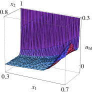
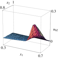
Figure 5: Stereographs of $u_{h1}^{n}$ (left) and $u_{h2}^{n}$ (right) at $t^{n}=8$ by Scheme LG^′ in Example 2 when $\nu=10^{-4}$

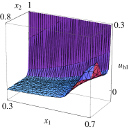
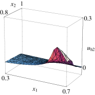
Figure 6: Stereographs of $u_{h1}^{n}$ (left) and $u_{h2}^{n}$ (right) at $t^{n}=8$ by Scheme LG-LLV in Example 2 when $\nu=10^{-4}$

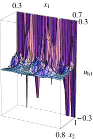
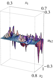
Figure 7: Stereographs of $u_{h1}^{n}$ (left) and $u_{h2}^{n}$ (right) at $t^{n}=8$ by Scheme LG^′ in Example 2 when $\nu=10^{-5}$

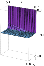
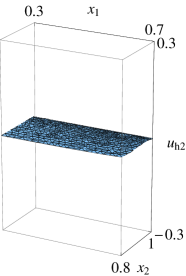
Figure 8: Stereographs of $u_{h1}^{n}$ (left) and $u_{h2}^{n}$ (right) at $t^{n}=8$ by Scheme LG-LLV in Example 2 when $\nu=10^{-5}$

Figure 4 (right) shows the triangulation of $\Omega$. Figures 5 and 6 show the stereographs of the solution $u_{h}^{n}$ at $t^{n}=8$ in the subdomain $(0.3,0.7)\times(0.8,1.0)$ by Scheme LG^′ and Scheme LG-LLV, respectively, when $\nu=10^{-4}$. Neither solution is oscillating although $u_{h2}$ of Scheme LG^′ takes larger values than that of Scheme LG-LLV. Figures 7 and 8 show the stereographs of the solution $u_{h}^{n}$ at $t^{n}=8$ in the subdomain $(0.3,0.7)\times(0.8,1.0)$ by Scheme LG^′ and Scheme LG-LLV, respectively, when $\nu=10^{-5}$. While oscillation is observed for both components of the solution by Scheme LG^′ in Figure 7, we can see that the solution by Scheme LG-LLV is solved without any oscillation in Figure 8.

7 Conclusions

We have present a Lagrange–Galerkin scheme free from numerical quadrature for the Navier–Stokes equations. By virtue of the introduction of a locally linearized velocity, the scheme can be implemented exactly and the theoretical stability and the convergence results are assured for practical numerical solutions. We have shown optimal error estimates in $\ell^{\infty}(H^{1})\times\ell^{2}(L^{2})$-norm for the velocity and pressure in the case of $\mathrm{P}_{2}/\mathrm{P}_{1}$- and $\mathrm{P}_{1}\mathrm{+}/\mathrm{P}_{1}$-finite elements. Numerical results have reflected these estimates and the robustness of the scheme for high-Reynolds number problems.

- (1) Achdou, Y., Guermond, J.: Convergence analysis of a finite element projection/Lagrange–Galerkin method for the incompressible Navier–Stokes equations. SIAM Journal on Numerical Analysis 37(3), 799–826 (2000)
- (2) Arnold, D., Brezzi, F., Fortin, M.: A stable finite element for the Stokes equations. CALCOLO 21(4), 337–344 (1984)
- (3) Bercovier, M., Pironneau, O.: Error estimates for finite element method solution of the Stokes problem in the primitive variables. Numerische Mathematik 33(2), 211–224 (1979)
- (4) Bermejo, R., del Sastre, P., Saavedra, L.: A second order in time modified Lagrange–Galerkin finite element method for the incompressible Navier–Stokes equations. SIAM Journal on Numerical Analysis 50(6), 3084–3109 (2012)
- (5) Boukir, K., Maday, Y., Métivet, B., Razafindrakoto, E.: A high-order characteristics/finite element method for the incompressible Navier-Stokes equations. International Journal for Numerical Methods in Fluids 25(12), 1421–1454 (1997)
- (6) Ciarlet, P.G.: The Finite Element Method for Elliptic Problems. Classics in Applied Mathematics. SIAM (2002)
- (7) Clément, P.: Approximation by finite element functions using local regularization. RAIRO Analyse numérique 9(2), 77–84 (1975)
- (8) Douglas Jr., J., Russell, T.: Numerical methods for convection-dominated diffusion problems based on combining the method of characteristics with finite element or finite difference procedures. SIAM Journal on Numerical Analysis 19(5), 871–885 (1982)
- (9) Girault, V., Raviart, P.A.: Finite Element Methods for Navier-Stokes Equations. Springer Berlin Heidelberg (1986)
- (10) Hammer, P.C., Marlowe, O.J., Stroud, A.H.: Numerical integration over simplexes and cones. Mathematics of Computation 10, 130–137 (1956)
- (11) Hecht, F.: New development in FreeFem++. Journal of Numerical Mathematics 20(3-4), 251–265 (2012)
- (12) Morton, K.W., Priestley, A., Süli, E.: Stability of the Lagrange-Galerkin method with non-exact integration. Mathematical Modelling and Numerical Analysis 22(4), 625–653 (1988)
- (13) Notsu, H., Tabata, M.: A single-step characteristic-curve finite element scheme of second order in time for the incompressible Navier-Stokes equations. Journal of Scientific Computing 38(1), 1–14 (2009)
- (14) Notsu, H., Tabata, M.: Error estimates of a stabilized Lagrange-Galerkin scheme for the Navier-Stokes equations (2015). ArXiv: [math.NA]
- (15) Pironneau, O.: On the transport-diffusion algorithm and its applications to the Navier-Stokes equations. Numerische Mathematik 38, 309–332 (1982)
- (16) Pironneau, O., Tabata, M.: Stability and convergence of a Galerkin-characteristics finite element scheme of lumped mass type. International Journal for Numerical Methods in Fluids 64(10-12), 1240–1253 (2010)
- (17) Priestley, A.: Exact projections and the Lagrange-Galerkin method: a realistic alternative to quadrature. Journal of Computational Physics 112(2), 316–333 (1994)
- (18) Rui, H., Tabata, M.: A second order characteristic finite element scheme for convection-diffusion problems. Numerische Mathematik 92, 161–177 (2002)
- (19) Süli, E.: Convergence and nonlinear stability of the Lagrange-Galerkin method for the Navier-Stokes equations. Numerische Mathematik 53(4), 459–483 (1988)
- (20) Tabata, M.: Discrepancy between theory and real computation on the stability of some finite element schemes. Journal of computational and applied mathematics 199(2), 424–431 (2007)
- (21) Tabata, M., Fujima, S.: Robustness of a characteristic finite element scheme of second order in time increment. In: Computational Fluid Dynamics 2004, pp. 177–182. Springer (2006)
- (22) Tabata, M., Uchiumi, S.: A genuinely stable Lagrange–Galerkin scheme for convection-diffusion problems. arXiv (2015). 1505.05984v1 [math.NA]
- (23) Tanaka, K., Suzuki, A., Tabata, M.: A characteristic finite element method using the exact integration. Annual Report of Research Institute for Information Technology Kyushu University 2, 11–18 (2002). (in Japanese)
- (24) Verfürth, R.: Error estimates for a mixed finite element approximation of the Stokes equations. RAIRO Analyse numérique 18(2), 175–182 (1984)