Adiabatic approximation and fluctuations in exciton-polariton condensates

Abstract

We study the relation between the models commonly used to describe the dynamics of nonresonantly pumped exciton-polariton condensates, namely the ones described by the complex Ginzburg-Landau equation, and by the open-dissipative Gross-Pitaevskii equation including a separate equation for the reservoir density. In particular, we focus on the validity of the adiabatic approximation that allows to reduce the coupled condensate-reservoir dynamics to a single partial differential equation. We find that the adiabatic approximation consists of three independent analytical conditions that have to be fulfilled simultaneously. By investigating stochastic versions of the two corresponding models, we verify that the breakdown of the adiabatic approximation can lead to discrepancies in correlation lengths and distributions of fluctuations. Additionally, we consider the phase diffusion and number fluctuations of a condensate in a box, and show that self-consistent description requires treatment beyond the typical Bogoliubov approximation.

I Introduction

Exciton-polaritons are coherent superpositions of quantum well excitons and a microcavity photons, resulting from strong coupling of the two modes at resonance Hopfield (1958); Weisbuch et al. (1992); Kavokin et al. (2007). The mixed nature of these quasiparticles is attractive from the point of view of fundamental and applied research in many ways. The matter component provides strong interactions, while the photonic component yields very light effective mass and allows for straightforward detection. Condensation and supefluidity of polaritons or polariton lasing has been demonstrated in many laboratories, even at room temperature Amo et al. (2009); Lagoudakis et al. (2008); Carusotto and Ciuti (2013); Kasprzak et al. (2006); Christopoulos et al. (2007); Kéna-Cohen and Forrest (2010); Plumhof et al. (2014); Deng et al. (2010).

In the case of nonresonant pumping, polaritons can be created either using a beam at frequency above the polariton resonance or using electrical carrier injection Schneider et al. (2013). Free carriers and high-energy excitons undergo energy relaxation towards the polariton ground state, where they can condense Kasprzak et al. (2006). Theoretical description of this complicated process, involving scattering with phonons and other polaritons is a formidable task, and several approaches have been proposed in the past with various approximations involved Haug et al. (2014); Wouters and Savona (2009); Solnyshkov et al. (2014); Laussy et al. (2004); Galbiati et al. (2012); Tassone et al. (1997). Among these, phenomenological models based on various generalizations of the Gross-Pitaevskii equation Keeling and Berloff (2008); Wouters and Carusotto (2007); Wouters et al. (2010) have been particularly useful thanks to their simplicity and limited number of external parameters. The most commonly used are the complex Ginzburg-Landau equation (CGLE, also termed the generalized GP equation in some works), with a single equation for the condensate evolution, and the open-dissipative Gross-Pitaevskii equation (ODGPE, other names are also used in the literature) Wouters and Carusotto (2007), which attempts to describe the full system dynamics using a pair of coupled condensate-reservoir equations. It has been pointed out in several places Dreismann et al. (2014); Berloff and Keeling (2013); Altman et al. (2015) that the ODGPE model can be reduced to the CGLE model under the adiabatic (quickly responding reservoir) approximation, but the validity of this approximation has not been investigated in detail.

In this paper, we investigate systematically the relation between the the CGLE the ODGPE models. We establish precisely conditions under which the reduction to the CGLE model is justified; contrary to the common belief, we show that the fast reservoir relaxation alone is not a sufficient condition. We show that adiabaticity requires three independent analytical conditions to be fulfilled simultaneously. Additionally, the condensate must remain close to the steady state, since large fluctuations may lead to complete breakdown of the correspondence between the models. Such large fluctuations occur in particular close to the condensation/stability limits of the condensate phase diagram.

In the second part of the paper, we investigate how the breakdown of the adiabaticity influences the steady state solutions of the corresponding stochastic CGLE/ODGPE models. Recently, fluctuations of nonequilibrium quantum fluids became a very active area of research. Spatial Chiocchetta and Carusotto (2013); Gladilin et al. (2014a) and temporal Ji et al. (2015); He et al. (2014) correlations have been investigated in the small fluctuations regime, and the critical scaling properties have been established using the renormalization group Sieberer et al. (2013, 2014); He et al. (2014). Dynamics of the polariton condensation phase transition have been shown to display similarities with the Kibble-Zurek theory of universal dynamics Matuszewski and Witkowska (2014); Liew et al. (2015). Here, we show how the spectrum of fluctuations and spatial correlations are modified in the non-adiabatic regime as well as in the large fluctuations regime. In particular, we demonstrate the appearance of dark soliton-like structures and chaotic bistable steady states close to the limits of condensate stability in parameter space in the ODGPE model.

In addition, we consider a model of a condensate in a box, in which case condensation may occur despite the absence of true long-range order at low dimensions Mora and Castin (2003); Petrov et al. (2004); Chiocchetta and Carusotto (2013). We show that a self-consistent description requires treatment beyond the typical Bogoliubov approximation, and demonstrate how the zero-momentum singularity of the momentum distribution spectrum Chiocchetta and Carusotto (2013) can be avoided by an appropriate generalization of the Bogoliubov ansatz. This allows for the determination of the number fluctuations and condensate phase diffusion equation.

The paper is organized as follows. In Sec. II we introduce the CGLE and ODGPE models as well as their stochastic versions, in particular the stochastic Gross-Pitaevskii (SGPE) model being a generalization of the CGLE. In Sec. III we derive carefully the conditions under which the adiabatic reduction of the ODGPE to the CGLE model is justified. In Sec. IV we recall briefly the main analytical results concerning the fluctuations and spatial correlations of the condensate. We also present the analysis of the fluctuations and phase diffusion of a condensate confined in a box. In Sec. V we present numerical investigation of the properties of stochastic steady states in various regimes. Sec. VI concludes the paper.

II Models

II.1 Complex Ginzburg-Landau equation

The simplest dissipative model to describe one-dimensional exciton-polariton condensates is the complex-Ginzburg-Landau equation (CGLE)

$$i\textrm{d}\phi= \left[A-B\nabla^{2}+C|\phi|^{2}+i\left(D-E|\phi|^{2}\right)\right]\phi\,{\rm d}t+$$

$$+ {\rm d}W_{\rm CGLE},$$ (1)

where for future reference we additionally included the stochastic term ${\rm d}W_{\rm CGLE}({\bf x},t)$ which vanishes in the classical limit. The real parameters of the equation describe the energy offset ($A$), the dispersion coefficient ($B$), nonlinear interactions ($C$), external pumping ($D$), and nonlinear losses ($E$). In the case of interest the parameters $B$, $C$, $D$ and $E$ are positive, which guarantees the existence of a stable homogeneous solution $\phi({\bf x},t)=\phi_{0}e^{-i\mu t}=\sqrt{D/E}e^{-i\mu t}$ with $\mu=A+C|\phi_{0}|^{2}$  van Saarloos and Hohenberg (1992). Compared to the most general form of the CGLE, we assume no diffusive term (as $B$ is real), although models including the diffusive term have also been employed Wertz et al. (2012); Keeling and Berloff (2008); Sieberer et al. (2013). It is, however, not crucial to our considerations. We note that the coefficient $A$ can be removed simply by moving to a rotating frame where $\phi^{\prime}({\bf x},t)=\phi({\bf x},t)e^{iAt}$, provided that the noise is not time-correlated.

A generalized form of the CGLE, or the stochastic Gross-Pitaevskii equation (SGPE), has been used in several works which investigated spatial correlations of the condensate Wouters and Carusotto (2007); Chiocchetta and Carusotto (2013)

$$i\textrm{d}\phi = \left[\omega_{0}-\frac{\hbar}{2m_{0}^{*}}\nabla^{2}+g_{0}|\phi|^{2}\right.+$$

$$+ \left.i\left(\frac{P_{0}}{1+\frac{|\phi|^{2}}{n_{s}}}-\gamma_{0}\right)\right]\phi\,\textrm{d}t+\textrm{d}W_{\rm SGPE},$$

where $\phi({\bf x},t)$ is the wave function, $m_{0}^{*}$ is the effective mass of lower polaritons, $g_{0}$ is the interaction coefficient, $\omega_{0}$ is the oscillation frequency, $P_{0}$ is the pumping rate, $\gamma_{0}$ is the polariton loss rate, $n_{s}$ is the saturation density, and $\textrm{d}W_{\rm SGPE}({\bf x},t)$ is the complex stochastic noise.

As in the second part of the manuscript we will focus on the spatial correlations, we will compare our results to the above model (II.1), which was used in Wouters and Carusotto (2007); Chiocchetta and Carusotto (2013), rather than the standard CGLE (II.1). These two models are, however, completely equivalent as long as one is interested in a state with small density fluctuations around the homogeneous solution. To show this consider the solution for which the density can be written as $|\phi({\bf x},t)|^{2}=|\phi_{0}|^{2}+\delta n$, where $\delta n/|\phi_{0}|^{2}\ll 1$. The fraction in Eq. (II.1) can be expanded in Taylor series, and by neglecting second- and higher-order terms in $\delta n$ we obtain Eq. (II.1) with the correspondence $A=\omega_{0}$, $B=\hbar/2m_{0}^{*}$, $C=g_{0}$, $D=\gamma_{0}-(\gamma_{0}^{2}/P_{0})$, $E=\gamma_{0}^{2}/n_{s}P_{0}$, $\textrm{d}W_{\rm CGLE}=\textrm{d}W_{\rm SGPE}$, which yields the steady state density $|\phi_{0}|^{2}=n_{s}(P_{0}-\gamma_{0})/\gamma_{0}$ for $P_{0}>\gamma_{0}$.

For completeness, we note that in Wouters and Carusotto (2007); Chiocchetta and Carusotto (2013) the stochastic noise was assumed to be Gaussian with the correlations

$$\langle\textrm{d}W_{\rm SGPE}({\bf x})\textrm{d}W_{\rm SGPE}^{*}({\bf x}^{\prime})\rangle =2D_{\phi\phi}\delta({\bf x}-{\bf x}^{\prime})\textrm{d}t,$$

$$\langle\textrm{d}W_{\rm SGPE}({\bf x})\textrm{d}W_{\rm SGPE}({\bf x}^{\prime})\rangle =0$$ (3)

and the amplitude $D_{\phi\phi}\approx\gamma_{0}$, which is an estimate of the quantum noise due to the dissipative coupling. Since the above white noise $\textrm{d}W_{\rm SGPE}$ has a diverging norm, in practice an appropriate UV cutoff must be employed eg. through frequency dependence of the amplification term Chiocchetta and Carusotto (2013). Alternatively, one may model the process on a discretized mesh with lattice constant $\Delta x$, where the Dirac delta is replaced as $\delta({\bf x}-{\bf x}^{\prime})\rightarrow\delta_{{\bf x},{\bf x}^{\prime}}/(\Delta x)^{d}$. We note that an alternative form of stochatic noise was derived from a quantum model of condensation in a cavity interacting with two-level emitters Chiocchetta and Carusotto (2014).

II.2 Open-dissipative Gross-Pitaevskii equation

A more realistic model of the polariton condensate, called the open-dissipative Gross-Pitaevskii equation (ODGPE), includes coupling of the condensate wave function to the reservoir described by a density field $n_{\rm R}({\bf x},t)$  Wouters and Carusotto (2007); Wouters and Savona (2009)

$$i\textrm{d}\psi= \left[-\frac{\hbar}{2m^{*}}\nabla^{2}+g_{C}|\psi|^{2}+g_{R}n_{R}+\right.$$ (4)

$$\left.+\frac{i}{2}\left(Rn_{R}-\gamma_{C}\right)\right]\psi\textrm{d}t+\textrm{d}W,$$

$$\frac{\partial n_{R}}{\partial t}= P-\left(\gamma_{R}+R|\psi|^{2}\right)n_{R},$$ (5)

where the complex stochastic noise can be obtained within the truncated Wigner approximation Wouters and Savona (2009)

$$\langle\textrm{d}W({\bf x})\textrm{d}W^{*}({\bf x}^{\prime})\rangle =\frac{\textrm{d}t}{2(\Delta x)^{d}}(Rn_{R}+\gamma_{C})\delta_{{\bf x},{\bf x}^{\prime}},$$ (6)

$$\langle\textrm{d}W({\bf x})\textrm{d}W({\bf x}^{\prime})\rangle =0.$$ (7)

where we assumed a constant scattering rate $R$ which gives noise correlations analogous as in Eq. (II.1). Here $P({\bf x})$ is the exciton creation rate determined by the pumping profile, $\gamma_{\rm C}$ and $\gamma_{\rm R}$ are the polariton and reservoir loss rates, and $R$ is the rate of stimulated scattering from the reservoir to the condensate, and $g_{\rm C}$, $g_{\rm R}$ are the rates of repulsive polariton-polariton and reservoir-polariton interactions, respectively.

In the absence of noise, a spatially uniform solution is given by $\psi({\bf x},t)=\psi_{0}e^{-i\mu_{0}t}$, $n_{R}({\bf x},t)=n_{R}^{0}$. Above the threshold pumping $P>P_{\rm th}=\gamma_{C}\gamma_{R}/R$ a stable condensate exists with the condensate density $|\psi_{0}|^{2}=(P/\gamma_{C})-(\gamma_{R}/R)$, $n_{R}^{0}=\gamma_{C}/R$, and $\mu_{0}=g_{C}|\psi_{0}|^{2}+g_{R}n_{R}^{0}$. We note that formally similar models were also used to describe nonlinear effects in semiconductor microcavities at weak coupling Taranenko et al. (2005)and atom lasers Kneer et al. (1998). The above phenomenological model has been successful in describing a number of different experimental situations in exciton-polariton condensates, although various values of parameters have been used in the literature Bobrovska et al. (2014); Wertz et al. (2012); Lagoudakis et al. (2011); Roumpos et al. (2010).

III Adiabatic approximation and the correspondence between the models

III.1 Adiabatic limit

The open-dissipative Gross-Pitaevskii model Eqs. (4)-(5) can be reduced to the simpler and more tractable CGLE model Eq. (II.1) under the assumption that the reservoir density $n_{\rm R}({\bf x},t)$ adiabatically follows the change of $|\psi({\bf x},t)|^{2}$. With the use of Eq. (5) we can express $n_{\rm R}$ as

$$n_{\rm R}({\bf x},t)=\frac{P}{\gamma_{R}+R|\psi({\bf x},t)|^{2}}.$$ (8)

Note that the above relation is valid also in the case of a stationary state $n_{\rm R}({\bf x},t)=n_{\rm R}({\bf x})$, $\psi({\bf x},t)=\psi({\bf x})e^{-i\mu t}$, regardless of the adiabatic assumption. However, in this work we are interested in dynamical processes and the limits of validity of the adiabatic approximation. The Eq. (4) now takes the form of a generalized CGLE

$$i\textrm{d}\psi = \left[-\frac{\hbar}{2m_{0}}\nabla^{2}+g_{C}|\psi|^{2}+\frac{g_{R}P}{\gamma_{R}+R|\psi({\bf x},t)|^{2}}\right.+$$ (9)

$$+ \left.\frac{i}{2}\left(\frac{RP}{\gamma_{R}+R|\psi({\bf x},t)|^{2}}-\gamma_{C}\right)\right]\psi\,\textrm{d}t+\textrm{d}W.$$

Again, this equation is equivalent to Eqs. (II.1) and (II.1), provided that the condensate density $|\psi({\bf x},t)|^{2}$ is close to the homogeneous solution $|\psi_{0}|^{2}=(P/\gamma_{C})-(\gamma_{R}/R)$ which allows for expansion of the right hand side in Taylor series to the first order. We emphasize that the expansion is done around the steady state density, and not zero density of the condensate. As will be shown in subsection V.3, at low density (pumping slightly above threshold) the results of the two models disagree qualitatively due to large fluctuations. The full correspondence between the three models is given by

$$A=\omega_{0}=g_{R}\left(\frac{2\gamma_{C}}{R}-\frac{\gamma_{C}^{2}\gamma_{R}}{R^{2}P}\right),$$

$$B=\frac{\hbar}{2m_{0}^{*}}=\frac{\hbar}{2m^{*}},$$

$$C=g_{0}=g_{C}-g_{R}\frac{\gamma_{C}^{2}}{RP},$$ (10)

$$D=\gamma_{0}-\frac{\gamma_{0}^{2}}{P_{0}}=\frac{\gamma_{C}}{2}-\frac{\gamma_{C}^{2}\gamma_{R}}{2PR},$$

$$E=\frac{\gamma_{0}^{2}}{n_{s}P_{0}}=\frac{\gamma_{C}^{2}}{2P},$$

$$D_{\phi\phi}=\gamma_{0}=\gamma_{C}/2.$$

Note that there are only six equations while seven parameters are present in the open-dissipative model. Consequently, one free parameter can be chosen when calculating seven parameters of Eqs. (4)-(5) corresponding to six parameters of Eq. (II.1) or Eq. (II.1). In the classical limit (no stochastic noise) the last equation is absent and there is an additional free parameter in both Eqs. (4)-(5) and Eq. (II.1).

III.2 Validity of the adiabatic approximation

The limits of the validity of the adiabatic approximation can be estimated by comparing the characteristic timescales existing in the dynamical system. To this end consider Eqs. (4)-(5) and assume that the adiabatic approximation is fulfilled; the reservoir density $n_{\rm R}$ is able to quickly adjust to the condensate density $|\psi|^{2}$ which changes on a much longer timescale. Equation (5) has a simple solution if $|\psi({\bf x},t)|^{2}$ is treated as a constant

$$n_{\rm R}({\bf x},t)=\frac{P}{\gamma_{R}+R|\psi({\bf x},t)|^{2}}+Ce^{-(\gamma_{R}+R|\psi({\bf x},t)|^{2})t}.$$ (11)

Therefore the timescale of the reservoir is $\tau_{R}=(\gamma_{R}+R|\psi({\bf x},t)|^{2})^{-1}$. For the adiabatic assumption to be consistent, this timescale must be much smaller than the timescales of the condensate, which are given by all the four terms in Eq. (4). We obtain four conditions that, if fulfilled simultaneously, give a sufficient condition for the validity of the adiabatic approximation; namely, all the terms $\frac{\hbar k^{2}}{2m^{*}}$, $\frac{1}{2}|Rn_{R}-\gamma_{C}|$, $g_{C}|\psi|^{2}$, and $g_{R}n_{R}$ must be much smaller than $\tau_{R}^{-1}=\gamma_{R}+R|\psi|^{2}$. The first condition means that only the low momentum modes of the condensate

$$k^{2}\ll 2m^{*}/(\hbar\tau_{R})$$ (12)

may be occupied considerably. The other conditions provide relations between the system parameters, as we show below.

We now make the same assumption that was used to compare the different models of the condensate, expressing the condensate density as a steady state value plus small fluctuations, $|\phi({\bf x},t)|^{2}=|\phi_{0}|^{2}+\delta n$. Under this assumption, the second of the above conditions is always fulfilled. The third and fourth conditions take the simple forms

$$\frac{P_{\rm th}}{P}\gg\frac{g_{C}-R}{g_{C}},$$ (13)

$$\frac{P}{P_{\rm th}}\gg\frac{g_{R}}{R}\frac{\gamma_{C}}{\gamma_{R}}.$$ (14)

Equation (13) is always true if $g<R$, and otherwise it gives an upper limit for the pumping $P$. Equation (14) gives a lower limit for $P$. Note that the condition (13) is independent of the reservoir relaxation rate $\gamma_{R}$.

Finally, we note that while the above conditions are sufficient, but not necessary, it is unlikely that if one of the four terms is large, it could be fully compensated by another term in Eq. (4), since the terms depend very differently on the fields $n_{\rm R}$ and $\psi$. We also emphasize once again that Eqs. (13) and (14) as well as the exact correspondence between the models are only valid if the condensate density is close to the steady state value.

III.3 Limits of modulational stability

It is well known that the CGLE (II.1) displays linear modulational instability (also called Benjamin-Feir instability) for $BC<0$, which is a special case of the Benjamin-Feir-Newell criterion Aranson and Kramer (2002); van Saarloos and Hohenberg (1992). While the dispersion coefficient $B$ is always positive in our model, it follows from Eqs. (10) that not all choices of the interaction coefficients $g_{C}>0$ and $g_{R}>0$ correspond to a positive value of $C$. A simple application of Eqs. (10) yields the criterion for linear stability

$$\frac{P}{P_{\rm th}}>\frac{g_{R}}{g_{C}}\frac{\gamma_{C}}{\gamma_{R}}.$$ (15)

In other words, the violation of the stability condition (15) corresponds to effectively attractive interactions in the CGLE or SGPE model, $C,g_{0}<0$. The above instability of the model (4)-(5) was first reported in Wouters and Carusotto (2007), where it was named the “hole-burning effect”, and the analytical condition for stability (15) was first derived in Smirnov et al. (2014) by investigation of the Bogoliubov-de Gennes excitation spectrum. Alternatively, the same condition can be derived from the analysis of the total blueshift originating from both $g_{C}$ and $g_{R}$ Liew et al. (2015).

IV Fluctuations and spatial correlations

In the rest of the paper, we investigate how the breakdown of the adiabatic approximation influences the fluctuations around the steady state and spatial correlation functions. We first recall the relevant results of Chiocchetta and Carusotto (2013) and Gladilin et al. (2014b) corresponding to the SGPE (or adiabatic) case. We also derive self-consistently analytical formulas for the number fluctuations and phase diffusion of a condensate in a finite box. In the last section we present numerical results in both the adiabatic and non-adiabatic regimes.

IV.1 Previous analytical results

In Chiocchetta and Carusotto (2013) Bogoliubov-de Gennes equations for the small fluctuations around the condensate in the form $\phi({\bf x},t)=\left[\phi_{0}+\delta\phi({\bf x},t)\right]e^{-i\mu t}$ were used to determine the momentum distribution of the particles in the SGPE model (II.1). The number of particles in each mode in the steady state was calculated as

$$n^{ss}_{\textbf{k}}=(2\pi)^{d}|\phi_{0}|^{2}\delta^{(d)}(\textbf{k})+\frac{D_{\phi\phi}}{\Gamma}\left[\frac{\mu^{2}+\Gamma^{2}}{E^{2}_{\textbf{k}}}+1\right],$$ (16)

where $\Gamma=\gamma_{0}(P_{0}-\gamma_{0})/P_{0}$ is the effective damping rate, $\mu=g_{0}|\phi_{0}|^{2}>0$ is the energy of interactions between particles, and $E^{2}_{\textbf{k}}=\epsilon_{\textbf{k}}(\epsilon_{\textbf{k}}+2\mu)$ with $\epsilon_{\textbf{k}}=\hbar k^{2}/2m^{*}$ is the Bogoliubov dispersion. The first term on the right hand side corresponds to the condensate, and the second term to the non-condensed cloud.

The formula (16) must be used with caution. It displays both the IR divergence in the $E^{-2}_{\textbf{k}}$ term and the UV divergence in the constant term. While the UV divergence can be healed in the case of frequency-dependent pumping Chiocchetta and Carusotto (2013) or discretization of the system on a lattice, the IR divergence poses a problem for the interpretation of the above formula at the $k=0$ point. We show below how this problem can be solved by an appropriate generalization of the Bogoliubov approximation.

Notice also that in the infinite system (“thermodynamic” limit with $V\rightarrow\infty$ at constant pumping) the fraction of particles in the condensate vanishes in the relevant one- and two-dimensional cases Chiocchetta and Carusotto (2013), invalidating the Bogoliubov approximation. However, the long-range correlations are mostly influenced by the phase fluctuations, which are much less energetically costly than the amplitude fluctuations due to the existence of a Goldstone mode of phase twists Mora and Castin (2003); Petrov et al. (2004). The correlations are accurately described using the density-phase generalized Bogoliubov approximation $\phi({\bf x},t)=\sqrt{n_{0}+\delta n}\,e^{i\theta({\bf x},t)-i\mu t}$, which yields the long-range correlations in one dimension falling exponentially as Chiocchetta and Carusotto (2013); Gladilin et al. (2014b)

$$g^{(1)}(x)\sim\exp(-x/l_{1}),\quad{\rm where}\quad l_{1}=\frac{2n_{0}\hbar\mu\Gamma}{mD_{\phi\phi}(\mu^{2}+\Gamma^{2})}.$$ (17)

IV.2 Condensate in a box

In a finite system where ${\bf k}$ is discretized, the fraction of particles in the condensate $k=0$ can be large, and we will consider this case in this subsection. In the following we consider a condensate in a box of length $L$ and periodic boundary conditions with $\Delta k=2\pi/L$, for which we have the correspondence $\delta^{(d)}(\textbf{k})\rightarrow(L/(2\pi))^{d}\delta_{k,0}$. The first term on the right hand side of (16) can be written simply as $(2\pi)^{d}|\phi_{0}|^{2}\delta^{(d)}(\textbf{k})=|\phi_{0}|^{2}L^{d}\delta_{k,0}\equiv N_{0}\delta_{k,0}$. To cope with the IR divergence due to the singularity at $k=0$ we introduce a generalized density-phase Bogoliubov Ansatz which takes into account the diffusion of the condensate phase $\varphi(t)$

$$\phi({\bf x},t)=\left[\phi_{0}+\delta\phi_{k=0}(t)\right]e^{i\varphi(t)-i\omega t}+\delta\phi_{k\neq 0}({\bf x},t),$$ (18)

where $\varphi(t)$ and $\delta\phi_{k=0}(t)$ are real functions describing the phase and amplitude fluctuations of the condensate, and $\delta\phi_{k\neq 0}({\bf x},t)$ is a complex function describing the fluctuations in the out-of-condensate modes. In contrast to the standard Bogoliubov approach, we treat the fluctuations of the $k=0$ mode in a special way. We do not assume that the phase $\varphi(t)$ is a small quantity, but allow it to undergo a Brownian-like motion under the action of the stochastic noise Scully and Zubairy (1997). Substituting the above into Eq. (II.1) and going into Fourier space, the fluctuations $\delta\tilde{\phi}_{k\neq 0}(k,t)$ separate from $\delta\tilde{\phi}_{k=0}(t)$ and $\varphi(t)$ in the linearized limit. One gets a set of equations

$$\frac{d\,\delta\phi_{k=0}}{dt} =-2\Gamma\,\delta\phi_{k=0}+\frac{1}{L^{d/2}}\frac{dW_{I,k=0}}{dt},$$ (19)

$$\frac{d\varphi}{dt} =-\frac{1}{\sqrt{N_{c}}}\left(2\mu L^{d/2}\,\delta\phi_{k=0}+\frac{dW_{R,k=0}}{dt}\right),$$ (20)

where $N_{c}(t)=L^{d}|\phi_{0}+\delta\phi_{k=0}|^{2}$ and we split the noise into the real and imaginary part with $\langle dW_{R,I,k=0}dW^{*}_{R,I,k=0}\rangle=D_{\phi\phi}dt$. Equation (19) corresponds to the Ornstein-Uhlenbeck process while Eq. (20) describes phase diffusion. By stochastic integration of the first equation Gardiner (1983) we calculate the number fluctuations in the condensate

$$\Delta n_{k=0}=2N_{0}\sqrt{\frac{\langle\delta\phi_{k=0}^{2}\rangle}{\phi_{0}^{2}}}=\sqrt{\frac{D_{\phi\phi}N_{0}}{\Gamma}}.$$ (21)

As usual for an interacting condensate, the number fluctuations scale with the square root of $N_{0}$. The mean number of particles in the condensate and out-of-condensate modes is given by (recall that $N_{0}=|\phi_{0}|^{2}L^{d}$)

$$n^{ss}_{\textbf{k}}=\begin{cases}N_{0}+\frac{D{\phi\phi}}{4\Gamma}&\text{for }k=0,\\ \frac{D_{\phi\phi}}{\Gamma}\left[\frac{\mu^{2}+\Gamma^{2}}{E_{k}^{2}}+1\right]&\text{for }k\neq 0,\end{cases}$$ (22)

which should be compared with Eq. (16). The singularity at $k=0$ has been removed in Eq. (22), but an additional term $D_{\phi\phi}/4\Gamma$ indicates that on average the noise slightly increases the number of particles in the condensate.

For consistency, the size of the box must be sufficiently small so that the fraction of particles in the $k=0$ mode is considerable. The number of particles in out-of-condensate modes can be estimated by replacing the sum of $n^{ss}_{\textbf{k}}$ over $k$ by an integral over the modes from $\Delta k$ to $k_{\rm max}=2\pi/L$. From this estimate we get the self-consistency “small box” condition to be $L\ll\frac{4\pi^{2}\hbar|\phi_{0}|^{2}}{mD_{\phi\phi}}\frac{\Gamma\mu}{\Gamma^{2}+\mu^{2}}$ in the 1D case and $L\ln\frac{\mu mL^{2}}{\hbar\pi^{2}}\ll\frac{8\pi^{2}\hbar|\phi_{0}|^{2}}{mD_{\phi\phi}}\frac{\Gamma\mu}{\Gamma^{2}+\mu^{2}}$ in the 2D case.

V Numerical results

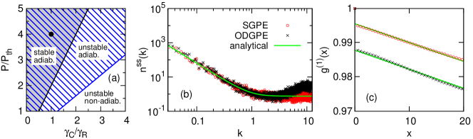
Figure 1: (Color online).  Stable and adiabatic regime. Left panel shows the position of the system on the stability-adiabaticity diagram. The black line corresponds to the stability condition (15) and the blue line to the adiabaticity condition (14). Middle panel shows momentum distribution in the steady state $n^{ss}(k)=|\psi(k)|^{2}\Delta k$ for both models compared to the analytical prediction from (16), (22). On the right panel the calculated first-order correlation functions $g^{(1)}(x)$ are displayed together with the analytical long-range fit (17). Parameters in dimensionless ODGPE units (23) are $R=1$, $g_{C}=0.4$, $g_{R}=2g_{C}$, $P/P_{\rm th}=4$, $\gamma_{C}=1$, $\gamma_{R}=1$, $\beta=0.003$, $L=600$.

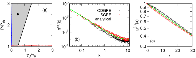
Figure 2: (Color online).  Stable and non-adiabatic regime. Same as in Fig. 1, except for $g=20$, $g_{R}=2g$, $P/P_{\rm th}=2.5$, $\gamma_{C}=0.5$.

In this subsection we investigate in detail the effects of the breakdown of the adiabatic approximation on the momentum distribution and spatial correlation functions of a one-dimensional condensate. To this end we investigate numerically the steady states of the system using both the 1D version of the SGPE model (II.1) and the open-dissipative Gross-Pitaevskii model (4)-(5) with the fluctuations included. We compare these numerical results with the analytical predictions given by (16), (17) and (22).

To investigate the breakdown of adiabaticity we consider various values of parameters for which the adiabaticity conditions (13) and (14) are either fulfilled or not. We clearly observe that the two models lead to the same results only in the adiabatic regime. We also find that the discrepancy between the SGPE and ODGPE models may be caused by large density fluctuations, which also invalidate the correspondence between the models. This behaviour is observed close to the limits of condensate stability (15) and $P=P_{\rm th}$.

Note that in the one-dimensional case the nonlinear coefficients scale with the confinement strength, eg. $(R^{\rm 1D},g_{i}^{\rm 1D})=(R^{\rm 2D},g_{i}^{\rm 2D})/\sqrt{2\pi d^{2}}$, if we assume a Gaussian transverse profile of $|\psi|^{2}$ and $n_{\rm R}$ of width $d$. In the case of a one-dimensional microwire Wertz et al. (2010), the profile width $d$ is of the order of the microwire thickness. For convenience we also introduce dimensionless parameters in the system (4)-(5) which allows us to describe the system using a limited set of parameters. By rescaling time, space, wave function amplitude and material coefficients as $t=\tau\widetilde{t}$, $x=\xi\widetilde{x}$, $\psi=(\xi\beta)^{-1/2}\widetilde{\psi}$, $n_{R}=(\xi\beta)^{-1}\widetilde{n}_{R}$ $R^{\rm 1D}=(\xi\beta/\tau)\widetilde{R}$, $(g^{\rm 1D},g_{R}^{\rm 1D})=(\hbar\xi\beta/\tau)(\widetilde{g},\widetilde{g}_{R})$, $(\gamma_{C},\gamma_{R})=\tau^{-1}(\widetilde{\gamma_{C}},\widetilde{\gamma}_{R})$, $P(x)=(1/\xi\beta\tau)\widetilde{P}(x)$, where $\xi=\sqrt{\hbar\tau/2m^{*}}$, while $\tau$ and $\beta$ are arbitrary scaling parameters, we can rewrite the above equation in the dimensionless form (from now on we omit the tildas for convenience)

$$i\frac{\partial\psi}{\partial t}=\left[-\frac{\partial^{2}}{{\partial x}^{2}}+\frac{i}{2}\left(Rn_{R}-\gamma_{C}\right)+g_{C}|\psi|^{2}+g_{R}n_{R}\right]\psi,$$

$$\frac{\partial n_{R}}{\partial t}=P-\left(\gamma_{R}+R|\psi|^{2}\right)n_{R},$$ (23)

In particular, we may choose the time scaling $\tau$ in such a way that $\gamma_{R}=1$ without loss of generality. The norms of both fields $N_{\psi}=\int|\psi|^{2}dx$ and $N_{R}=\int n_{R}dx$ are scaled by the factor of $\beta$, and the noise correlators become $\langle dW(x)dW^{*}(x^{\prime})\rangle=\beta\frac{dt}{2\Delta x}(Rn_{R}+\gamma_{C})\delta_{x,x^{\prime}}$. The parameters of the SGPE model (II.1) can be rescaled in an analogous way.

The numerical simulations were performed on a grid of length $L=600$ with spatial step size $\Delta x=0.133$. We solved the equation (II.1) and (4)-(5) with the corresponding parameters given by the conditions (10). We compared the calculated momentum distribution $n^{ss}(k)$ and the first-order correlation function $g^{(1)}(x)$ in the steady state after long time evolution, starting from the initial state with $\phi(x,t=0)=\phi_{0}$ and $n_{\rm R}(x,t=0)=\gamma_{C}/R$. We found that typically the result does not depend on the initial conditions. However, for certain values of parameters, close to the stability threshold (15), an empty initial state $\phi(x,0)=0$ led to a qualitatively different evolution (see the next subsection for details).

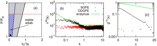
Figure 3: (Color online). Steady state close to the condensation threshold, exhibiting large fluctuations. Same as in Fig. 1, except $g=2.5$, $g_{R}=2g$, $P/P_{\rm th}=1.05$, $\gamma_{C}=0.1$.

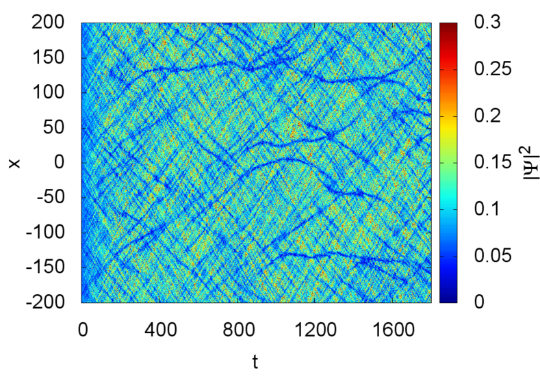
Figure 4: (Color online). Density evolution corresponding to Fig. 3, revealing dark solitons in the dynamical steady state of the ODGPE.

V.1 Stable-adiabatic regime

In Figure 1 we show the results in the stable-adiabatic case, i.e. for parameters fulfilling both the stability (15) and adiabaticity conditions (13)-(14). The left panel shows the position on the phase diagram. The middle panel displays the numerically obtained momentum distribution $n^{ss}(k)=|\psi(k)|^{2}\Delta k$ from 15 simulations of both models, compared with the analytical prediction of the momentum “tail” ($k>0$) of (16) and (22). While the numerical box size $L$ is so large that we are in a quasicondensate rather than condensate regime Chiocchetta and Carusotto (2013), and the fraction of particles at $k=0$ is very small, the momentum tail distribution closely follows the analytical predictions. This follows from the fact that in the quasicondensate regime the Bogoliubov approximation can still be applied to a slice of the system where the quasicondensate phase is approximately constant.

The discrepancy between the SGPE and ODGPE models is visible only at high momenta, where the first (momentum-dependent) adiabaticity condition (12) breaks down. Indeed, this condition gives the upper limit $k\ll 8$ , which coincides with the value of $k$ at which the ODGPE results start to deviate from the SGPE and analytical predictions. We note that this limit corresponds to very high momentum values.

On the other hand, the $g^{(1)}(x)$ function follows the analytically predicted long-range trend (17) very closely for both models. The difference between the two is in the different value of the constant in front of the exponent in (17), which can be again attributed to the breakdown of adiabaticity at very high momenta, related to short distances.

Further, we performed a series of numerical tests in the stable-adiabatic regime with other values of parameters. With increasing ratio $\gamma_{C}/\gamma_{R}$, moving towards the stability threshold (15), the differences between analytical and numerical results become more notable. Beyond the stability threshold, which corresponds to $g_{0}=0$, the comparison is no longer possible since the analytical formulas are valid only for the case of repulsive effective interactions, $g_{0}>0$.

V.2 Stable-nonadiabatic regime

Figure 2 shows the results in the stable-nonadiabatic case, when the adiabaticity conditions (13) and (14) are not fulfilled. In this case we increased the strength of the interactions $g_{C}$ and $g_{R}$. There is a visible discrepancy between the models both in the momentum distribution and the first-order correlation function, which marks the breakdown of the adiabatic approximation. Note that the results are presented in the logarithmic scale, and the actual difference between the calculated averages of $n^{ss}(k)$ differ significantly. The SGPE result still follows the Bogoliubov analytical prediction closely. The correlation function only slightly differs from the analytical prediction for both models, as shown in the right panel.

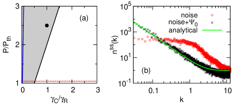
Figure 5: (Color online). System close to the stability threshold. In the right panel momentum distributions obtained from different initial conditions are shown (see text). Parameters are as in Fig. 2, except $\gamma_{C}=1$.

V.3 Large fluctuations

Importantly, as shown in previous sections, the adiabaticity conditions (12)-(14) are valid only under the assumption that the system is in a steady state with small fluctuations. Moreover, without this assumption the reduction of the generalized CGLE (9) to the CGLE or SGPE models is not possible. We illustrate the situation in which the fluctuations are large in Fig. 3, where the pumping was chosen slightly above the threshold value $P\approx P_{\rm th}$. In this case even the generalized Bogoliubov approximations are not relevant and the analytical predictions are incorrect. Moreover, the results provided by the SGPE and ODGPE models are qualitatively different. The SGPE model predicts momentum distribution $n^{ss}(k)$ that is practically independent of momentum and negligible spatial correlations. On the other hand, the ODGPE predicts a nontrivial momentum distribution and decaying $g^{(1)}(x)$ indicating an appearance of a finite spatial correlation length, not related to the Bogoliubov prediction (17).

We associate this spatial length scale with the spontaneous appearance of dark structures depicted in Fig. 4. The figure shows density distribution in one randomly chosen realization of the truncated Wigner stochastic evolution (4)-(5), which can be interpreted as a single realization of the experiment Wouters and Savona (2009); Matuszewski and Witkowska (2014). The structures appear to be related to dark solitons of the dissipative model Xue and Matuszewski (2014); Pinsker and Flayac (2014); Smirnov et al. (2014). We checked that each dark object corresponds to an approximate $\pi$ phase jump of the phase of $\psi(x,t)$. A detailed investigation of these excitations will be presented elsewhere.

V.4 Stability threshold and the role of initial conditions

In the majority part of the stability diagram, the initial conditions given as a seed to the evolution do not influence the steady state properties. However, the situation is drastically different for the ODGPE model in the vicinity of the stability threshold given by (15). An example is given in Fig. 5. Here, the momentum distribution is plotted for simulations starting from two different initial conditions, either $\psi(x,t=0)=\psi_{0}+\xi(x)$ or $\psi(x,t=0)=\xi(x)$, where $\xi$ represents a small uncorrelated noise with a Gaussian distribution. In the first case, the system converges to a steady state that is very well described by the analytical Bogoliubov momentum distribution. In the second case, the system does not reach this state even after very long evolution, instead dwelling in a chaotic evolution with large density fluctuations. The “normal” and “chaotic” states are therefore metastable. This behavior can be generally observed in the vicinity of the stability limit, both on the stable and unstable side of the phase diagram of Fig. 5. We checked that this bistability persits even if a relaxation term (frequency-dependent pumping) is included the evolution equation (4), analogous as in Wouters and Carusotto (2010). Since we do not find any similar dynamics in the SGPE model, we conclude that it is also related to the breakdown of the adiabatic approximation. The investigation of these chaotic states will be a topic of a future study.

VI Conclusions

In conclusion, we investigated the relation between the models commonly used in the literature to describe nonresonantly pumped exciton-polariton condensates. The complex Ginzburg-Landau equation, and the equivalent (in the limit of small fluctuations) stochastic Gross-Pitaevskii equation were compared with the open-dissipative Gross-Pitaevskii equation which includes a separate equation for the reservoir density. The adiabatic approximation allows to reduce the latter to one of the single-equation models, under the assumptions that the condensate is close to the steady state and fluctuations are small. Additionally, three independent analytical conditions for adiabaticity must be met simultaneously. While spin degree of freedom was not taken into account in this work, the generalization to the spin-dependent case is straightforward.

We investigated the corresponding stochastic models by comparing the numerical steady states with the analytical predictions of the Bogoliubov approximation. We demonstrated how the zero-momentum singularity of the momentum distribution spectrum can be avoided by an appropriate generalization of the Bogoliubov approximation. This also allowed for determination of the number fluctuations and condensate phase diffusion equation.

The comparison of the models with and without a separate equation for the reservoir demonstrated that close agreement between the two can be obtained only under the adiabatic conditions. Moreover, we showed that close to the limit of condensation or the limit of modulational stability, large fluctuations lead to qualitatively different results depending on the model used. These results show that special care must be taken when choosing the right model for describing exciton-polariton condensates in certain conditions.